Any correspondence concerning this service should be sent
to the repository administrator:
[email protected]
This is an author’s version published in:
http://oatao.univ-toulouse.fr/24807
To cite this version: Hall, Neil and Köhler, Hemming and Link,
Sebastian and Prade, Henri
and Zhou, Xiaofang Cardinality
constraints on qualitatively uncertain data. (2015) Data and
Knowledge Engineering, 99. 126-150. ISSN 0169-023X
Official URL
DOI :
https://doi.org/10.1016/j.datak.2015.06.002
Open Archive Toulouse Archive Ouverte
OATAO is an open access repository that collects the work of Toulouse
researchers and makes it freely available over the web where possible
Cardinality constraints on qualitatively uncertain data
Neil Hall
a, Henning Koehler
b, Sebastian Link
a,⁎
, Henri Prade
c, Xiaofang Zhou
d,e aDepartment of Computer Science, The University of Auckland, New ZealandbSchool of Engineering & Advanced Technology, Massey University, New Zealand cIRIT, CNRS Université de Toulouse III, France
dSchool of Information Technology and Electrical Engineering, The University of Queensland, Australia eSoochow University, Suzhou, China
a b s t r a c t
Modern applications require advanced techniques and tools to process large volumes of uncertain data. For that purpose we introduce cardinality constraints as a principled tool to control the occurrences of uncertain data. Uncertainty is modeled qualitatively by assigning to each object a degree of possibility by which the object occurs in an uncertain instance. Cardinality constraints are assigned a degree of certainty that stipulates on which objects they hold. Our framework empowers users to model uncertainty in an intuitive way, without the requirement to put a pre-cise value on it. Our class of cardinality constraints enjoys a natural possible world semantics, which is exploited to establish several tools to reason about them. We characterize the associated implication problem axiomatically and algorithmically in linear input time. Furthermore, we show how to visualize any given set of our cardinality constraints in the form of an Armstrong sketch. Even though the problem of finding an Armstrong sketch is precisely exponential, our algorithm computes a sketch with conservative use of time and space. Data engineers may therefore com-pute Armstrong sketches that they can jointly inspect with domain experts in order to consolidate the set of cardinality constraints meaningful for a given application domain.
Keywords:
Data and knowledge visualization Data models
Database semantics
Management of integrity constraints Requirements engineering
1. Introduction 1.1. Background
The notion of cardinality constraints is fundamental for understanding the structure and semantics of data. In traditional concep-tual modeling, cardinality constraints were introduced in Chen's seminal paper[7]. They have attracted significant interest and tool support ever since. Intuitively, a cardinality constraint consists of a set of attributes and a positive integer b, and holds in an instance if there are no b + 1 distinct objects in the instance that have matching values on all the attributes of the constraint. For example, bank customers with no more than 5 withdrawals from their bank account per month may qualify for a special interest rate. Traditionally, cardinality constraints empower applications to control the occurrences of certain data, and therefore have significant applications in data cleaning, integration, modeling, processing, and retrieval.
1.2. Motivation
Traditional conceptual modeling was targeted at certain data for applications such as accounting, inventory and payroll. Modern applications, such as information extraction, radio-frequency identification (RFID), scientific data management, data cleaning, and
⁎ Corresponding author.
E-mail addresses:[email protected](N. Hall),[email protected](H. Koehler),[email protected](S. Link),[email protected](H. Prade),
[email protected](X. Zhou).
financial risk assessment produce large volumes of uncertain data. For example, RFID can track movements of endangered species of animals, such as the Indiana bat in Georgia, USA. For such an application, data comes in the form of objects associated with some discrete level of confidence in the signal reading; for example based on the quality of the signal received. More generally, uncertainty can be modeled qualitatively by associating objects with the degree of possibility (p-degree) that the object is perceived to occur in the instance.Fig. 1shows such a possibilistic instance (p-instance), where each object is associated with an element from a finite scale of p-degrees:α1N … N αk + 1. The top degreeα1is reserved for objects that are ‘fully possible’, the bottom degreeαk + 1for objects that are ‘impossible’ to occur. Intermediate degrees are used as required and linguistic interpretations attached as preferred, such as ‘quite possible’ (α2) and ‘somewhat possible’ (α3).
As this scenario is typical for a broad range of applications, we investigate in this article how cardinality constraints can benefit from the p-degrees assigned to objects. More specifically, we investigate cardinality constraints on uncertain data, where uncertainty is modeled qualitatively in the form of p-degrees.
The degrees of possibility are a natural source for extending the expressivity of traditional cardinality constraints. In fact, our use of p-degrees enjoys a natural possible world semantics, as illustrated on the running example inFig. 1. Here, the world w1contains the RFID readings of high quality only, that is, all the objects with p-degreeα1. The world w2contains RFID readings of high or good quality, that is, all the objects with p-degreeα1orα2. Finally, world w3contains RFID readings of high, good, or low quality, that is, all the objects with p-degreeα1,α2orα3. This possible world semantics enables us to express traditional cardinality constraints with different degrees of cer-tainty. The certainty by which a traditional cardinality constraint holds is derived from the possible worlds in which it holds.
For example, we can express that for all low, good, and high quality readings, there are at most three readings recorded in the same zone, by declaring the cardinality constraint card(Zone) ≤ 3 to be ‘fully certain’. That is, card(Zone) ≤ 3 must hold in the largest possible world w3, and therefore also in all the worlds it contains. Similarly, we can express that for all good and high quality readings, at most two bats are recorded in the same zone at the same time, by declaring the cardinality constraint card(Zone, Time) ≤ 2 to be ‘quite cer-tain’. That is, card(Zone, Time) ≤ 2 must hold in the second largest possible world w2, but not necessarily in the largest world w3. Finally, we can express that for all high quality readings, the zone and time together identify the bat, by declaring the cardinality constraint card(Zone, Time) ≤ 1 to be ‘somewhat certain’. That is, card(Zone, Time) ≤ 1 must hold in the smallest possible world w1, but not necessarily in the worlds w2or w3.
1.3. Contributions
Our objective is to apply possibility theory from artificial intelligence to establish qualitative cardinality constraints (QCs) as a fundamental tool to control the occurrences of uncertain data. Our contributions can be summarized as follows:
• Modeling. We introduce qualitative cardinality constraints as a class of integrity constraints on uncertain data. Here, uncertainty is modeled qualitatively by assigning to each object a degree of possibility with which it occurs in the instance. The p-degrees bring forward a nested chain of possible worlds, with each world being a classic instance that has some possibility. Hence, the higher the possibility of a world the fewer objects it contains. This empowers us to assign degrees of certainty to cardinality constraints, stipulating to which possible worlds they apply. The degrees of certainty (c-degree) are usually denoted byβ1N … N βkN βk + 1, whereβk + 1denotes the bottom c-degree reserved for constraints that are satisfied by any p-instance. Cardinality constraints that apply to the largest possible world hold with ‘full certainty’, denoted by the top c-degreeβ1, while cardinality constraints that apply to the smallest possible world are only ‘somewhat certain’ to hold, denoted by the c-degreeβk.Fig. 1shows the possible
Fig. 1. P-instance and its possible worlds as the result of integrating RFID readings of different qualities; Armstrong p-sketch of the qualitative cardinality constraints that the p-instance satisfies.
worlds w1, w2and w3of our running example. Here, w2satisfies card(Zone, Time) ≤ 2 but violates card(Zone, Time) ≤ 1, which holds only on world w1.
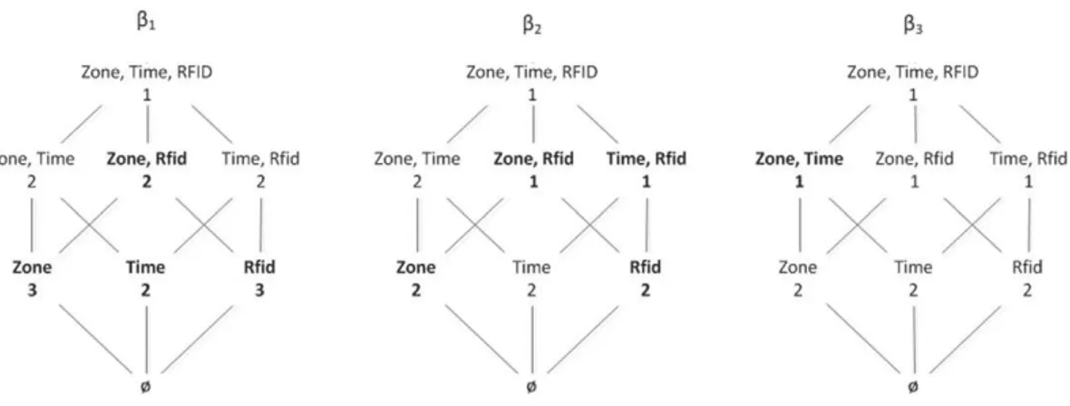
• Reasoning. We establish axiomatic and algorithmic solutions to the implication problem associated with qualitative cardinality constraints. The implication problem is to decide, for any given qualitative cardinality constraint and any set of such constraints over a given object type, whether the constraint is implied by the set, that is, whether every instance over the object type that satisfies every element of the set also satisfies the constraint. Technically, the algorithmic solution to the implication problem is derived from a linear-time characterization of the inference problem, where one must compute for any given traditional cardinality constraint and any given set of qualitative cardinality constraints on any given object type, the highest degree of certainty with which the constraint is implied by the given set. Our algorithmic solution allows us to detect and remove any redundant constraints from a given set, thereby reducing the number of cardinality constraints that must actively be enforced on given sets of objects to a minimal level necessary. This ability results in time savings proportional to the size of the data sets. That means our solutions empower us to efficiently enforce many desirable properties of uncertain data arising from modern application domains. For exam-ple,Fig. 2shows a cover for the qualitative cardinality constraints that the p-instance fromFig. 1satisfies. In the figure a qualitative cardinality constraint (card(X) ≤ b,β) is represented as follows: the cube under the c-degree β features all attribute sets X with the minimal upper bound b that applies to them. The constraints that form a minimal cover ∑ for the set of all qualitative cardinality constraints satisfied by the p-instance are shown in bold font. For example, the constraint (card(Time) ≤ 2, β2) is implied by the constraint (card(Time) ≤ 2,β1). We also show that our findings cannot only be used to control the integrity of uncertain data, but also have interesting applications to query processing. For example, our solution of the implication problem can be used to compute upper bounds on the number of query answers without actually having to query the potentially big data set.
• Acquisition. The benefits of applying qualitative cardinality constraints effectively to an application are inhibited by the difficulty of identifying those constraints that actually hold on the domain of the application. In the idealized special case where only fully certain objects occur in the data, it is already difficult to identify the correct upper bound. In the context of uncertain data, the problem becomes even more intricate as the correct degree of certainty has to be identified for any given upper bound. It is therefore impor-tant to provide computational support to business analysts who need to discover meaningful qualitative cardinality constraints. For this purpose, we investigate Armstrong samples for the class of qualitative cardinality constraints. A p-instance is said to be Armstrong for a given set of qualitative cardinality constraints if and only if for every qualitative cardinality constraint, it holds that it is implied by the given set if and only if it is satisfied by the p-instance. An Armstrong p-instance therefore tells us the highest degree of certainty by which a qualitative cardinality constraint is implied by the given set. While there are sets of qualitative cardinality constraints which require every Armstrong p-instance to be infinite, we show that every set of qualitative cardinality constraints enjoys Armstrong p-sketches, which are finite representations of potentially infinite Armstrong p-instances. Even though the problem of finding an Armstrong p-sketch is precisely exponential, we establish an algorithm that computes an Armstrong p-sketch with conservative use of time and space. Business analysts may therefore compute Armstrong p-sketches that they can jointly inspect with domain experts in order to consolidate the correct degree of certainty with which cardinality constraints should hold in the given application domain. For example, the p-instance fromFig. 1is a finite Armstrong p-instance for the set ∑ of qualitative cardinality constraints above. An Armstrong p-sketch for ∑ is shown on the right ofFig. 1. Although p-sketches are mostly useful to finitely represent infinite Armstrong p-instances, they are also more concise representations of finite Armstrong p-instances. They are more concise as they require fewer objects and focus the attention of the people who inspect them on only the relevant patterns of data. For instance, the row (Card:2, Zone:Z7, Time:*, RFID:R8,α3) summarizes the fact that any p-instance that the p-sketch represents must feature two different objects that both have the value Z7 on Zone, each have unique values on Time, both have the value R8 on RFID, and both have associated p-degreeα3.
• Tool support and experiments. We implemented our algorithm for computing Armstrong p-sketches in a prototype system, and con-ducted several experiments regarding the size of the output and the time to compute the sketches. Our prototype successfully transfers the concept of Armstrong p-sketches from theory into practice. Our results suggest that Armstrong p-sketches, as computed by our pro-totype, are small enough for effective use during the requirements acquisition phase, and can be computed very quickly.
In summary, we introduce a new class of cardinality constraint that is useful in terms of i) expressing the semantics of uncertain data within a given application domain, ii) the small effort required to reason about them and process updates and queries more efficiently, and iii) the computational support available to acquire them.
1.4. Organization
InSection 2we summarize briefly the vast research on cardinality constraints from the community. This points out the lack of qualitative approaches to constraints on uncertain data. We propose a semantics for qualitative cardinality constraints on instances of uncertain data inSection 3. InSection 4we establish axiomatic and linear-time algorithmic characterizations for the associated implication problem of qualitative cardinality constraints, and linear-time algorithmic characterizations for the associated inference problem. This section also features two applications of our results. The first application is an algorithm for computing a minimal cover for a given set of qualitative cardinality constraints, which can be used to determine a minimal set of constraints that must be enforced when updates are processed. The second application illustrates the usefulness of our results for processing queries.Section 5details how to visualize arbitrary sets of qualitative cardinality constraints in the form of Armstrong p-sketches. While the problem of finding an Armstrong p-sketch is shown to be precisely exponential, our computed Armstrong p-sketch is always at most quadratic in the size of a minimum-sized Armstrong p-sketch and the given set of constraints. We briefly present our prototype system inSection 6, and the results of our experiments inSection 7. In Section 8we conclude and discuss future work.
2. Related work
Cardinality constraints are one of the most influential contributions conceptual modeling has made to the study of database constraints. They were present in Chen's seminal paper[7]on conceptual database design. It is no surprise that today they are part of all major languages for data and knowledge modeling, including UML, EER, ORM, XSD, or OWL. Cardinality constraints have been extensively studied in database design[1,6,8,14,15,18,19,23–25,27,31,32,35,37,42,43]. For a recent survey, see[44].
There are many quantitative approaches to uncertain data, foremost probability theory[41]. Research about constraints on prob-abilistic data is still in its infancy[5,26,38]. Qualitative approaches to uncertain data deal with either query languages or extensions of functional dependencies[4]. In[28]we introduced the class of possibilistic keys on qualitatively uncertain data, established axiomatic and algorithmic characterizations of their associated implication problem, and showed how to construct finite Armstrong p-instances for them. Possibilistic keys can be expressed by qualitative cardinality constraints of the form (card(X) ≤ 1,β). In contrast to qualitative cardinality constraints, Armstrong p-instances for any set of possibilistic keys are guaranteed to be finite. Qualitative approaches to cardinality constraints on uncertain data have not been studied yet to the best of our knowledge. Our contributions extend results on cardinality constraints from traditional conceptual modeling, covered by the special case of two degrees of possibility. These include findings on the implication problem and Armstrong databases[20]. The definition of Armstrong p-sketches as finite representations of potentially infinite Armstrong p-instances is original.
Possibilistic logic is a well-established tool for reasoning about uncertainty[9,12]with numerous applications in artificial intelli-gence[11], including approximate reasoning[45], non-monotonic reasoning[16], qualitative reasoning [40], belief revision [10,17,36], soft constraint satisfaction problems[3], decision-making under uncertainty[39], and pattern classification and prefer-ences[2]. Our results show that possibilistic logic is suitable to extend the classical notion of cardinality constraints from certain to qualitatively uncertain data.
The current article is an extended version of the conference paper[29]. The extensions are manifold. 1) We introduce the new concept of Armstrong p-sketches. This concept is highly useful for the discovery of meaningful qualitative cardinality constraints because finite Armstrong p-sketches exist for any given set of these constraints. In contrast, there are sets of qualitative cardinality constraints that require infinite Armstrong p-instances. The conference paper[29]was restricted to the study of Armstrong p-instances only. As these are only finite in cases where for each underlying attribute some finite upper bound has been specified with full certainty, the use of Armstrong p-instances is limited in practice. Even in the case where a finite Armstrong p-instance does exist, an Armstrong p-sketch still provides a more concise summary. 2) We study the inference problem of qualitative cardinality constraints, which has not been considered in previous research. Our linear-time solution to this problem can also be used to decide the associated implication problem in linear time in the input. 3) We have included some applications of our results, notably an algo-rithm to compute some minimal cover for a given set of qualitative cardinality constraints and can be applied to enforce cardinality constraints on uncertain data without redundancy; as well as an example that illustrates the applications of our findings to query processing and cardinality estimation. 4) While the conference paper[29]did not include any proofs, we include all proofs in the current article. This not only makes it possible to understand the validity of our results and algorithms, but also provides all details for the techniques and constructions we establish. 5) A detailed running example is provided to illustrate the concepts and findings throughout the article. Our proofs and findings may become more accessible for the reader, or at least provide a showcase to which they are applied. 6) We have transferred the concept of Armstrong p-sketches from theory into practice by implementing our algorithm in a prototype system. 7) We conducted several experiments with our prototype, showing that Armstrong p-sketches are small enough to use them successfully during the requirements acquisition phase and can be computed very quickly with our prototype.
3. Qualitative cardinality constraints
In this section we extend object types that model certain objects in traditional conceptual modeling to model uncertain objects qualitatively. Based on our model to attribute to each object a degree of possibility with which it occurs, we can attribute degrees of certainty to traditional cardinality constraints that say to which objects they apply.
We start by recalling some basic definitions of attributes, object types, objects and their projections, and instances. An object type, denoted by O, is a finite non-empty set of attributes. Each attribute A ∈ O has a domain dom(A) of values. An object o over O is an element of the Cartesian product ∏A ∈ Odom(A). For X ⊆ O we denote by o(X) the projection of o on X. An instance over O is a setι of objects over O. Note that an instance may be infinite.
As our running example we use the object typeTRACKINGwith attributes Zone, Time, and Rfid. Objects either belong or do not belong
to an instance. For example, we cannot express that we have less confidence for the bat identified by Rfid value B5 to be in Zone Z5 at 01 am than for the same bat to be in Z4 at 12 am.
We model uncertain instances by assigning to each object some degree of possibility with which the object occurs in an instance. Formally, we have a possibility scale, that is, a finite strict linear order S ¼ ðS;bÞ with k + 1 elements, denoted by α1N ⋯ N αkN αk + 1. The elementsαi∈ S are called possibility degrees, or p-degrees for short. Here, α1is reserved for objects that are ‘fully possible’ to occur, whileαk + 1is reserved for objects that are ‘impossible’ to occur in an instance, and any intermediate p-degree might linguistically be interpreted by some graded version of possibility such as ‘somewhat possible’ or ‘rather possible’. Of course, a linguistic interpretation is not necessary at all. The use of a specific possibility scale should simply reflect the requirements of an organization to distinguish between different degrees of possibility with which it perceives its data to occur. In our running example, we choose k = 3 and interpretα1as ‘fully possible’,α2as ‘quite possible’,α3as ‘somewhat possible’, andα4as ‘impossible’, reflecting the perceived quality of the RFID readings. We point out that humans like to use simple scales in everyday life to communicate, compare, or rank. Here, simple means to classify items qualitatively rather than quantitatively by putting precise values on them. Finally, we point out that classical instances are subsumed by the special case where k = 1. Here, objects that are assigned p-degreeα1are the objects of the instance, while all objects that do not occur in the instance are assumed to be assigned p-degreeα2. As we demonstrate below, objects that are assigned the top p-degreeα1are not just ‘fully possible’ to occur, but in fact, ‘fully certain’ to occur as well. Therefore, classical instances are a special case of uncertain instances.
A possibilistic object type ðO;SÞ, or p-object type, consists of an object type O and a possibility scale S. A possibilistic instance, or p-instance, over ðO;SÞ consists of an instance ι over O, and a function Possιthat assigns to each object o ∈ι a p-degree PossιðoÞ∈
S−fαkþ1g. We sometimes omit Poss when denoting a p-instance.Fig. 1shows a p-instance over (TRACKING,S ¼ fα1;…;α4g). P-instances enjoy a possible world semantics. For i = 1, …, k let wiconsist of all objects inι that have p-degree at least αi, that is, wi= {o ∈ι|Possι(o) ≥αi}. Indeed, we have w1⊆ w2⊆ ⋯ ⊆ wk. The possibility distributionπιfor this linear chain of possible worlds is defined by πι(wi) =αi. Note that wk + 1is not a possible world, since its p-degreeπ(wk + 1) =αk + 1means ‘impossible’. Vice versa, Possι(o) for an object o ∈ι is the maximum p-degree max{αi|o ∈ wi} of a world to which o belongs. If o ∉ wk, then Poss(o) =αk + 1. Every object that is ‘fully possible’ occurs in every possible world, and is therefore also ‘fully certain’. Hence, instances are a special case of uncertain instances.Fig. 1shows the possible worlds w1⊊ w2⊊ w3of the p-instance in the same figure.
We introduce qualitative cardinality constraints, or QCs, as cardinality constraints that have some associated degree of certainty. As cardinality constraints are fundamental to applications with certain data, QCs will serve a similar role for applications with uncertain data. A cardinality constraint over object type O is an expression card(X) ≤ b where ∅ ≠ X ⊆ O and b is a positive integer. The cardinality constraint card(X) ≤ b over O is satisfied by an instance w over O, denoted by ⊨wcard(X) ≤ b, if there are no b + 1 distinct objects o1, …, ob + 1∈ w with matching values on all the attributes in X. For example,Fig. 1shows that card(Zone) ≤ 1 is not satisfied by any instance w1, w2or w3; card(Zone, Time) ≤ 1 is satisfied by w1, but not by w2nor w3; card(Rfid) ≤ 2 is satisfied by w1and w2, but not by w3; and card(Rfid) ≤ 3 is satisfied by w1, w2and w3.
The p-degrees of objects result in degrees of certainty by which QCs hold. As card(Rfid) ≤ 3 holds in every possible world, it is ‘fully certain’ to hold onι. As card(Rfid) ≤ 2 is only violated in a ‘somewhat possible’ world w3, it is ‘quite certain’ to hold onι. As the smallest world that violates card(Zone, Time) ≤ 1 is the ‘quite possible’ world w2, it is ‘somewhat certain’ to hold onι. As card(Zone) ≤ 1 is violated in the ‘fully possible’ world w1, it is ‘not certain at all’ to hold onι.
Similar to the scale S of p-degrees αifor objects we use a scale STof certainty degreesβj, or c-degrees, for cardinality constraints.
As indicated in the last paragraph, we use ‘fully certain’, ‘quite certain’, ‘somewhat certain’, and ‘not certain at all’ in our running example. Formally, the correspondence between p-degrees in S and the c-degrees in STis defined by the mapping αi↦βk + 2 − i
for i = 1, …, k + 1. Hence, the certainty Cι(card(X) ≤ b) by which the cardinality constraint card(X) ≤ b holds on the uncertain instance ι is either the top degree β1if card(X) ≤ b is satisfied by wk, or the minimum among the c-degreesβk + 2 − ithat correspond to possible worlds wiin which card(X) ≤ b is violated, that is,
Cιðcard Xð Þ≤bÞ ¼ β1 ; if ⊨w
kcard Xð Þ≤b
min βkþ2−ij⊭wicard Xð Þ≤b
n o
;otherwise (
:
Whenι denotes the p-instance fromFig. 1, then the c-degree Cι(card(Rfid) ≤ 3) isβ1as card(Rfid) ≤ 3 is even satisfied in the world w3. Similarly, the c-degree Cι(card(Rfid) ≤ 2) isβ2as the smallest possible world that violates card(Rfid) ≤ 2 is w3. The c-degree Cι(card(Zone, Time) ≤ 1) isβ3as the smallest possible world that violates card(Zone, Time) ≤ 1 is w2. Finally, the c-degree Cι(card(Zone) ≤ 1) isβ4as the smallest possible world that violates card(Zone, Time) ≤ 1 is w1.
We can now define the syntax and semantics of qualitative cardinality constraints.
Definition 1. Let ðO;SÞ denote a p-object type. A qualitative cardinality constraint (QC) over ðO;SÞ is an expression (card(X) ≤ b, β) where card(X) ≤ b denotes a cardinality constraint over O andβ∈ST. A p-instance (ι, Possι) over ðO;SÞ satisfies the QC (card(X) ≤ b, β) if and only if
Cι(card(X) ≤ b) ≥β.
Qualitative cardinality constraints form a class of integrity constraints tailored to uncertain data. Indeed, a QC (card(X) ≤ b,βi) separates semantically meaningful from meaningless p-relations by allowing violations of the cardinality constraint card(X) ≤ b only by objects with a p-degreeαjwhere j ≤ k + 1 − i. For i = 1, …, k, the c-degreeβiof (card(X) ≤ b,βi) means that the cardinality constraint card(X) ≤ b must hold in the possible world wk + 1 − i. This constitutes a conveniently flexible mechanism to enforce the targeted level of integrity effectively.
Example 1. Let Σ denote the set consisting of the following qualitative cardinality constraints: (card(Zone) ≤ 3,β1), (card(Time) ≤ 2,β1), (card(Rfid) ≤ 3, β1), (card(Zone, Rfid) ≤ 2, β1), (card(Zone) ≤ 2, β2), (card(Rfid) ≤ 2, β2), (card(Zone, Rfid) ≤ 1, β2), (card(Time, Rfid) ≤ 1,β2), (card(Zone, Time) ≤ 1,β3). The p-instanceι fromTable 3satisfies all of these QCs. However,ι violates (card(Rfid) ≤ 2,β1), (card(Rfid) ≤ 1,β2), and (card(Zone, Time) ≤ 1,β2).
4. Reasoning about qualitative cardinality constraints
In this section we will establish tools to reason about qualitative cardinality constraints. These subsume existing tools for the rea-soning about traditional cardinality constraints as the special case where only two p-degrees are used. We will introduce implication and inference problems as core problems associated with the reasoning about qualitative cardinality constraints. We will then estab-lish a theorem that allows us to reduce any instance of the implication problem for qualitative cardinality constraints to an instance of the implication problem for traditional cardinality constraints. This result will be used to establish a finite axiomatization for the implication of qualitative cardinality constraints by a simple set of Horn axioms. These axioms will allow us to establish a linear-time algorithm for solving the inference problem, which can also be used to decide the implication problem in linear linear-time. Finally, we will show that efficient integrity enforcement and query processing are two major areas in which our results can be applied. 4.1. Implication and inference problems
We first define two core problems associated with the reasoning about qualitative cardinality constraints. For this purpose, let Σ ∪ {φ} denote a set of QCs over ðO;SÞ. As we will show later, we can always assume without loss of generality that this set isfinite. We say that ∑ (finitely) impliesφ, denoted by Σ ⊨(f)φ, if and only if every (finite) p-instance (ι, Possι) over ðO;SÞ that satisfies every QC in ∑ also satisfies φ. In other words, there is no (finite) p-instance (ι, Possι) over ðO;SÞ that satisfies every QC in ∑ but violates φ. We use Σ(f)∗ = {φ|Σ ⊨(f)φ} to denote the (finite) semantic closure of ∑. The (finite) implication problem for QCs is to decide, given any p-object type, and any set Σ ∪ {φ} of QCs over the p-object type, whether Σ ⊨(f)φ holds.
Our first observation is that the finite implication problem and the implication problem coincide for the class of qualitative cardinality constraints. That is, for every object type and every set Σ ∪ {φ} of QCs over that object type, it is true that Σ ⊨ φ if and only it is true that Σ ⊨(f)φ.
Theorem 1. Finite and unrestricted implication problem coincide for the class of qualitative cardinality constraints. Proof. Let Σ ∪ {φ} denote a finite set of QCs over object type ðO;SÞ.
If ∑ impliesφ, then it follows immediately that ∑ finitely implies φ since every finite p-instance is also a p-instance.
It remains to show the following: if ∑ does not implyφ, then ∑ does not finitely imply φ. Let φ = (card(X) ≤ b, ≥ βi) and suppose that Σ ⊭φ. Hence, there must be some (possibly infinite) p-instance (ι, Possι) over ðO;SÞ that satisfies all QCs in ∑ and violatesφ. Consequently, there must be b + 1 distinct objects o1, …, ob + 1∈ ι such that Possι(oj) ≥αk + 1 − iholds for all j = 1, …, b + 1, and oi(X) = oj(X) holds for all 1 ≤ i ≤ j ≤ b + 1. Let ðιf;PossιfÞ denote thefinite p-instance over ðO;SÞ where ιf= {o1, …, ob + 1} and PossιfðojÞ ¼ PossιðojÞ for all j = 1, …, b + 1. By construction, ðιf;PossιfÞ isfinite and violates φ. In addition,
ðιf;PossιfÞ also satisfies every QC in ∑ since ιf⊆ ι holds and (ι, Possι) satisfies every QC in ∑. We have just shown that ∑ does
not finitely imply φ, which completes the proof. □
PROBLEM: (Finite) Implication problem for qualitative cardinality constraints INPUT: Object type ðO;SÞ,
Finite set Σ ∪ {φ} of QCs over ðO;SÞ OUTPUT: Yes, if Σ ⊨(f)φ; No, otherwise
Theorem 1allows us to speak of the implication problem of qualitative cardinality constraints.
Example 2. Let ∑ be as inExample 1. Further, letφ denote the QC (card(Rfid) ≤ 2, β1). Then ∑ does not implyφ as the following p-instance witnesses:
We now return to our previous claim that we can assume without loss of generality that a given set ∑ of qualitative cardinality constraints over a given object type is finite. In a nutshell, for each fixed attribute set X and each c-degree βiit only matters which smallest upper bound bXi
is given to us. If ∑ is infinite, then there must be some infinite subset of ∑ of the form ΣX,i= {(card(X) ≤ bj,βi) ∈ Σ}. In this case, however, we can replace ΣX,iin ∑ by the singleton (card(X) ≤ bXi,βi) where bXi= min{bj|(card(X) ≤ bj,βi) ∈ ΣX,i}. If Σfdenotes the result of replacing for every non-empty X ⊆ O and every i = 1, …, k, ΣX,iby the singleton (card(X) ≤ bXi,βi), then ∑ implies every elements of Σfand Σfimplies every element of ∑. That is, Σfis a cover of ∑, which is finite. In particular, the semantic closure Σ∗
of a given ∑ of QCs is always infinite, but has a finite cover by the construction above. We may therefore assume without loss of generality that a set of qualitative cardinality constraints is given in the form of a finite cover.
While the implication problem is a decision problem, qualitative cardinality constraints also have an interesting computational problem associated with them. Given a set ∑ of QCs and a traditional cardinality constraint card(X) ≤ b, we may ask what the max-imum c-degreeβ is, with which (card(X) ≤ b, β) is implied by ∑. This is the inference problem of qualitative cardinality constraints.
Note that the inference problem also has a finite and unrestricted version, which both coincide due toTheorem 1.
Example 3. Let ∑ be as inExample 1. Then the maximum c-degree with which card(Rfid) ≤ 2 is implied by ∑ isβ2. In fact,Example 2has shown that (card(Rfid) ≤ 2,β1) is not implied by ∑, and (card(Rfid) ≤ 2,β2) ∈ Σ.
In what follows we will establish an axiomatic characterization of the implication problem, from which we will derive algorithmic characterizations of the inference and implication problems.
4.2. The magic ofβ-cuts
We will now establish a strong correspondence between instances of the implication problem for qualitative cardinality constraints and instances of the implication problem for cardinality constraints.
Definition 2. Let ∑ denote a set of qualitative cardinality constraints over the possibilistic object typeðO;SÞ. For each c-degree β∈S
Twhere
β N βk + 1, let Σβdenote those cardinality constraints card(X) ≤ b over object type O for which there is some (card(X) ≤ b,β′) ∈ Σ where β′ ≥ β, that is, Σβ¼ card Xð Þ ≤ bj card X$ ð Þ ≤ b;β0 % ∈ Σ and β0 ≥ β & ' :
We call Σβtheβ-cut of ∑.
For the set ∑ of QCs fromExample 1, the following cardinality constraints form theβ2-cut of ∑: card(Zone) ≤ 3, card(Time) ≤ 2, card(Rfid) ≤ 3, card(Zone, Rfid) ≤ 2, card(Zone) ≤ 2, card(Rfid) ≤ 2, card(Zone, Rfid) ≤ 1, and card(Time, Rfid) ≤ 1.
It turns out thatβ-cuts suffice to decide the implication problem for qualitative cardinality constraints, as the following theorem establishes.
Theorem 2. Let Σ ∪ {(card(X) ≤ b,β)} be a QC set over ðO;SÞ where β N βk + 1. Then Σ ⊨ (card(X) ≤ b,β) if and only if Σβ⊨ card(X) ≤ b. Proof. Suppose (ι, Possι) is some p-instance over ðO;SÞ that satisfies ∑, but violates (card(X) ≤ b, β). In particular, Cι(card(X) ≤ b) b β implies that there is some world withat violates card(X) ≤ b and whereβk + 2 − ib β.
Let card(Y) ≤ b′ ∈ Σβ, where (card(Y) ≤ b′,β′) ∈ Σ. Since ι satisfies (card(Y) ≤ b′, β′) ∈ Σ we have Cι(card(Y) ≤ b′) ≥β′ ≥ β. If wiviolated card(Y) ≤ b′, thenβ N βk + 2 − i≥ Cι(card(Y) ≤ b′) ≥β, a contradiction. Hence, wisatisfies Σβand violates card(X) ≤ b.
Zone Time Rfid Poss. degree Z3 11 pm B5 α1
Z4 12 am B5 α1
Z5 01 am B5 α3
PROBLEM: Inference problem for qualitative cardinality constraints INPUT: Object type ðO;SÞ,
Finite set ∑ of QCs over ðO;SÞ, and Cardinality constraint card(X) ≤ b over O OUTPUT: maxfβ∈STjΣ⊨ðcardðXÞ≤b;βÞg
Letι′ denote some instance that satisfies Σβand violates card(X) ≤ b, without loss of generalityι′ = {o1, …, ob + 1}. Letι be the p-instance over ðO;SÞ that consists of ι′ and where Possι(o1) = … = Possι(ob) =α1and Possι(ob + 1) =αi, such thatβk + 1 − i=β. Thenι violates (card(X) ≤ b, β) since Cι(card(X) ≤ b) =βk + 2 − i, as wi=ι′ is the smallest world that violates card(X) ≤ b, and βk + 2 − ib βk + 1 − i=β. For (card(Y) ≤ b′, β′) ∈ Σ we distinguish two cases. If wisatisfies card(Y) ≤ b′, then Cι(card(Y) ≤ b′) =β1≥ β. If wiviolates card(Y) ≤ b′, then card(Y) ≤ b′ ∉ Σβ, i.e.,β′ b β = βk + 1 − i. Therefore,β′ ≤ βk + 2 − i= Cι(card(Y) ≤ b′) as wi=ι′ is the smallest world that violates card(Y) ≤ b′. We conclude that Cι(card(Y) ≤ b′) ≥β′. Consequently, (ι, Possι) is a p-instance that satisfies
Σ and violates (card(X) ≤ b,β). □
Theorem 2allows us to apply achievements from cardinality constraints for certain data to qualitative cardinality constraints. It is a major tool to establish the remaining results in this article.
Example 4. Let Σ be as inExample 1. Then Σβ1consists of the cardinality constraints card(Zone) ≤ 3, card(Time) ≤ 2, card(Rfid) ≤ 3 and
card(Zone, Rfid) ≤ 2.Theorem 2says that Σβ1does not imply card(Rfid) ≤ 2. The possible world w3of the p-instance fromExample 2:
satisfiesΣ, and violates card(Rfid) ≤ 2. 4.3. Axiomatic characterization
In this section we will establish an axiomatic characterization for the implication problem of qualitative cardinality constraints by a finite set of Horn axioms. For this purpose, we first recall some basic definitions regarding axiomatizations.
In fact, we determine the semantic closure Σ∗of a set Σ of QCs by applying inference rules or axioms of the form premise
conclusion. In logic,
inference rules of this form are known as Horn axioms. For a set ℜ of inference rules let Σ ⊢ℜφ denote the inference of φ from Σ by ℜ. That is, there is some sequenceσ1, …,σnsuch thatσn=φ and every σiis an element of Σ or is the conclusion that results from an application of an inference rule in ℜ to some premises in {σ1, …,σi − 1}. Let Σℜ+= {φ|Σ ⊢ℜφ} be the syntactic closure of Σ under inferences by ℜ. ℜ is sound (complete) if for every set Σ over every p-object type ðO;SÞ we have Σℜ+⊆ Σ∗(Σ∗⊆ Σℜ+
). The (finite) set ℜ is a (finite) axiomatization if ℜ is both sound and complete.Table 1shows an axiomatization ℭ′ for the implication problem of traditional cardinality constraints[21]. In these rules, it is assumed that O is an arbitrarily given object type, X, Y ⊆ O are non-empty and b a positive integer.Theorem 2and the fact that ℭ′ forms a finite axiomatization for the implication of cardinality constraints can be exploited to show directly that the set ℭ fromTable 2forms an axiomatization for the implication of QCs. Here, it is assumed that ðO;SÞ is an arbitrarily given p-object type, X, Y ⊆ O are non-empty, b a positive integer, andβ;β0∈STsome c-degrees. In particular,βk + 1
denotes the bottom certainty degree in ST.
Theorem 3. The set ℭ forms a finite axiomatization for the implication of qualitative cardinality constraints.
Proof. The soundness proof is straightforward. Let Σ denote a set of QCs over p-object type ðO;SÞ. Let (ι, Possι) denote a p-instance over ðO;SÞ. The soundness of the top axiom T follows from the fact that ι is a set of objects over O and can therefore not contain any duplicate objects. Consequently, card(O) ≤ 1 holds with c-degreeβ1(and therefore with any other c-degree). For the soundness of the relax axiom ℛ suppose that (ι, Possι) satisfies (card(X) ≤ b, βi). That is the instance wk + 1 − isatisfies card(X) ≤ b. Since ℛ′ is sound for the implication of cardinality constraints, wk + 1 − ialso satisfies card(X) ≤ b + 1, which means that (ι, Possι) satisfies (card(X) ≤ b + 1,βi). For the soundness of the superset axiom S suppose that (ι, Possι) satisfies (card(X) ≤ b, βi). That is the instance wk + 1 − isatisfies card(X) ≤ b. Since S0is sound for the implication of cardinality constraints, wk + 1 − i
also satisfies card(XY) ≤ b, which means that (ι, Possι) satisfies (card(XY) ≤ b, βi). Since for (card(X) ≤ b,βk + 1) to be satisfied by some p-instance there is no requirement that any possible world satisfies card(X) ≤ b, the bottom axiom ℬ is sound, too. Finally, for the soundness of the weakening axiom W assume that (ι, Possι) satisfies (card(X) ≤ b, βi). Consequently, wk + 1 − isatisfies card(X) ≤ b and every world that wk + 1 − icontains must also satisfy card(X) ≤ b, including wk + 1 − jfor every k ≥ j ≥ i. Hence, (ι, Possι) satisfies (card(X) ≤ b, βj) for everyβj≤ βi. This establishes the soundness of ℭ.
Table 1
Axiomatization ℭ0¼ fT0;R0;S0g of traditional cardinality constraints.
cardðOÞ≤1 ðtop;T0Þ cardðXÞ≤b cardðXÞ≤b þ 1 ðrelax; R0Þ cardðXÞ≤b cardðXYÞ≤b ðsuperset; S0Þ Zone Time Rfid Z3 11 pm B5 Z4 12 am B5 Z5 01 am B5
For completeness, we applyTheorem 2and the fact that ℭ′ axiomatizes the implication of cardinality constraints. Let ðO;SÞ be a p-object type with jSj ¼ k þ 1, and Σ ∪ {(card(X) ≤ b, β)} a QC set such that Σ ⊨ (card(X) ≤ b, β). We need to show that Σ⊢ℭ(card(X) ≤ b,β) holds.
For Σ ⊨ (card(X) ≤ b,βk + 1) we have Σ ⊢ℭ(card(X) ≤ b,βk + 1) by applying B. Let now β b βk + 1. From Σ ⊨ (card(X) ≤ b,β) we conclude Σβ⊨ card(X) ≤ b byTheorem 2. Since ℭ′ is complete for the implication of cardinality constraints, Σβ⊢ℭ0cardðXÞ≤b holds.
Let Σββ= {(card(Y) ≤ b′,β)|card(Y) ≤ b′ ∈ Σβ}. Thus, the inference of card(X) ≤ b from Σβusing ℭ′ can be turned into an inference of (card(X) ≤ b,β) from Σββby ℭ, simply by addingβ to each QC in the inference. Hence, whenever T0or S0is applied, one applies instead
T or S, respectively. Consequently, Σββ⊢ℭ(card(X) ≤ b,β). The definition of Σββensures that every QC in Σ β
βcan be inferred from Σ by applying W. Hence, Σββ⊢ℭ(card(X) ≤ b,β) means that Σ ⊢ℭ(card(X) ≤ b,β).
□ Algorithm 1. Inference
Example 5. Let Σ be as inExample 1. The QC (card(Zone, Rfid) ≤ 4,β2) is implied by Σ. Indeed, applying the superset rule S to (card(Zone) ≤ 3, β1) ∈ Σ results in (card(Zone, Rfid) ≤ 3, β1) ∈ Σℭ+
. Applying the relax rule ℛ to this QC results in (card(Zone, Rfid) ≤ 4,β1) ∈ Σℭ+. Finally, an application of the weakening rule W to the last QC results in (card(Zone, Rfid) ≤ 4, β2) ∈ Σℭ+. 4.4. Algorithmic characterization
In practice, the semantic closure Σ∗of a finite set Σ of QCs is infinite and even though there always is some finite cover, it is often unnecessary to determine all implied QCs. In fact, the implication problem for QCs has as input Σ ∪ {φ} and the question is whether Σ impliesφ. Computing Σ∗and checking whetherφ ∈ Σ∗
is hardly efficient. In fact, we will now establish a linear-time algorithm for com-puting the maximum c-degreeβ such that (card(X) ≤ b, β) is implied by Σ. The following theorem allows us to reduce the implication problem for QCs to a single scan of the input.
Theorem 4. Let Σ ∪ {(card(X) ≤ b,β)} denote a set of QCs over ðO;SÞ with jSj ¼ k þ 1. Then Σ implies (card(X) ≤ b, β) if and only if β = βk + 1, or X = O, or there is some (card(Y) ≤ b′,β′) ∈ Σ such that Y ⊆ X, b′ ≤ b and β′ ≥ β.
Proof. Theorem 2shows for i = 1, …, k that Σ implies (card(X) ≤ b,βi) if and only if Σβimplies card(X) ≤ b. It is easy to observe from the axiomatization ℭ′ of cardinality constraints that Σβimplies card(X) ≤ b if and only if O = X, or there is some card(Y) ≤ b′ ∈Σβsuch that Y ⊆ X and b′ ≤ b hold. As Σ implies (card(X) ≤ b,βk + 1), the theorem follows. □
Theorem 4enables us to designAlgorithm 1, which returns for a given cardinality constraint card(X) ≤ b the maximum c-degreeβ for which (card(X) ≤ b,β) is implied by a given set Σ of QCs over p-object type ðO;SÞ. If X = O, then we return β1due to the soundness
Table 2
Axiomatization ℭ ¼ fT;ℛ;S;ℬ;Wg of qualitative cardinality constraints.
ðcardðOÞ≤βÞ ðtop;T Þ ðcardðXÞ≤ b;βÞ ðcardðXÞ≤b þ 1;βÞ ðrelax;RÞ ðcardðXÞ ≤b;βÞ ðcardðXYÞ≤b;βÞ ðsuperset;SÞ ðcardðXÞb;βkþ 1Þ ðbottom;ℬÞ ðcardðXÞ≤b;βÞ ðcardðXÞ≤b;β0Þ ðweakening;WÞ β0≤ β
of the top axiom T . Otherwise, starting with β = βk + 1the algorithm scans all input QCs (card(Y) ≤ b′,β′) and sets β to β′ whenever β′ is larger than the currentβ, X contains Y and b′ ≤ b.
Theorem 5states the correctness ofAlgorithm 1, which follows fromTheorem 4, as well as the time complexity. Note that ||Σ|| denotes the sum of the total number of attributes and the logarithm of the associated c-degree’s index that occur in the QCs of Σ. Theorem 5. On inputððO;SÞ; Σ;cardðXÞ≤bÞ,Algorithm 1returns inOðjjΣ∪fðcardðXÞ≤b;βkþ1ÞgjjÞ time the maximum c-degree β for which
(card(X) ≤ b,β) is implied by Σ. Algorithm 2. Minimal Cover
Example 6. Let Σ be as inExample 1, and useAlgorithm 1to determine the maximum c-degreeβ for which QC (card(Rfid) ≤ 2, β) is implied by Σ. In fact,β becomes β2as soon as the QC (card(Rfid) ≤ 2,β2) is selected as part of the input Σ. This c-degree cannot be increased and is therefore the output.
Theorem 5allows us to decide the associated implication problem efficiently, too. Given ððO;SÞ; Σ;ðcardðXÞ≤b;β
0
ÞÞ as an input to the implication problem we can useAlgorithm 1to computeβ := max{β′′|Σ ⊨ (card(X) ≤ b, β′′)} and return an affirmative answer if and only ifβ′ ≤ β.
Corollary 1. The implication problem of qualitative cardinality constraints can be decided in linear time in the input. □ Example 7. Following on fromExample 6, let Σ be as inExample 1. Then the QC (card(Rfid) ≤ 2,β3) is implied by Σ. Indeed, the maximum c-degreeβ for which (card(Rfid) ≤ 2, β) is implied by Σ was determined as β2inExample 6. Sinceβ3≤ β2, the given QC is indeed implied.
4.5. Applications to integrity enforcement and query processing
We conclude this section with some applications of our results. Our first application is the computation of a minimal cover for a given set Σ of qualitative cardinality constraints.
Recall from before that a cover of the given set Σ is a set Σ′ of QCs such that everyσ′ ∈ Σ′ is implied by Σ and every σ ∈ Σ is implied by Σ′. In other words, Σ′ is a faithful representation of Σ. A cover Σ′ of Σ is said to be minimal if and only if there is no proper subset Σ′′ of Σ′ that is also a cover of Σ. In other words, a minimal cover Σ′ does not feature any QCsσ′ that are redundant with respect to Σ′, i.e., redundant in the sense thatσ′ is implied by Σ′ − {σ′}. Our algorithmic solution to the implication problem suggests the following strategy for computing a minimal cover of a given QC set Σ: scan, one by one, each elementσ ∈ Σ whether it is implied by Σ − {σ}, and removeσ from Σ if that is the case. The resulting subset of Σ is a minimal cover. This strategy is manifested inAlgorithm 2.
The upper time bound of the following theorem follows from the linear time complexity of the associated implication problem, as established in Corollary 1.
Theorem 6.Algorithm 2computes a minimal cover in time OðjjΣjj2Þ in the size of the input Σ of qualitative cardinality constraints. □
The importance of minimal covers results from their application in integrity enforcement. To guarantee that the objects resulting from updates against the given instance conform to the rules of the application, the resulting instance must be validated against the given set of business rules. The overhead for this enforcement of business rules can be optimized by removing redundant business rules. The optimization is indirectly proportional to the number of objects in the instance. That is, the more objects are in the instance the more time savings can be achieved by enforcing only non-redundant rules. For this purpose, a minimal cover is desirable. Example 8. Let Σ′ be the set of qualitative cardinality constraints represented inFig. 2. Recall that these form a cover of the qualitative cardinality constraints satisfied by the p-instance inFig. 1. Given Σ′,Algorithm 2may compute a minimal cover Σ of Σ′ as given in Example 1, or in other words, the qualitative cardinality constraints highlighted in bold font inFig. 2.
As our second application we demonstrate the benefit of qualitative cardinality constraints on query processing. Therefore, we simply add the attribute P-degree to the object typeTRACKINGwith attributes Zone, Time, and Rfid. Suppose we are interested in finding
out which bats have been tracked in which zone, but we are only interested in answers that come from ‘certain’ or ‘quite possible’ objects in the instance. A user might enter the following SQL query:
which removes duplicate answers. When applied to the p-instance fromFig. 1, the query returns the answers on the right. Our framework allows users to ask such queries having available the p-degrees of objects. Answers can be ordered according to the p-degree, which makes it possible for users to appreciate their significance. The example shows how our framework can be embedded with standard technology, here SQL. Finally, the QC card(Zone, Rfid) ≤ 1 holds with maximum c-degreeβ2. That is, {Zone, Rfid} forms a key on the world w2that contains fully certain and quite possible objects. Consequently, the DISTINCT clause becomes superfluous in the query above. A query optimizer, capable of reasoning about QCs, can remove the DISTINCT clause from the input query without affecting its output. This optimization saves response time when answering queries, as duplicate elimination is an expensive opera-tion and therefore not executed by default in SQL databases. Note that we do not view the enforcement of meaningful constraints as an overhead, but a requirement that is necessary in data processing. Qualitative cardinality constraints, and the ability to reason about them, have therefore direct applications to query processing. We illustrate this point by a further example. Suppose we have a provid-er answprovid-ering quprovid-eries on large data sets as a sprovid-ervice to customprovid-ers. The customprovid-er will only pay for the sprovid-ervice when the price is not too high, but the provider will only want to invoke the service for a paying customer. Our reasoning abilities can be used to determine a “quote” for the price of some queries in the form of an upper bound on the number of query answers without the need to evaluate the query at all. The query
will return at most two answers when evaluated on any data set conforming to the set Σ of rules fromExample 1. The reason is that the qualitative cardinality constraint (card(Zone, Time) ≤ 2,β2) is implied by Σ. Being able to decide implication in linear time of the con-straints not only makes this feedback to the customer very efficient in practice, but also very affordable to the provider.
5. Armstrong samples for qualitative cardinality constraints
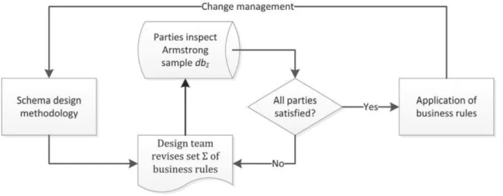
In this section we develop a theory of Armstrong samples for sets of qualitative cardinality constraints. The concept of an Armstrong database is well established in database research[13]. They are widely regarded as an effective tool to visualize abstract sets of con-straints in a user-friendly way[13,33,34]. As such data engineers exploit Armstrong databases as a communication tool in their interac-tion with domain experts in order to determine the set of constraints that are meaningful to the applicainterac-tion at hand[22,30,33,34]. As Fig. 3illustrates, a design team generates an Armstrong sample dbΣthat perfectly represents their current perceptions of the set Σ of con-straints that should be enforced. The team then jointly inspects the sample with domain experts in order to discover flaws or shortcom-ings in the perception of the design team. Evidently, the Armstrong sample helps designers and domain experts communicate more effectively, thereby overcoming the mismatch in expertise[30]. This process repeats until all parties are happy.
We now introduce the concept of an Armstrong p-instance for qualitative cardinality constraints. While we show that Armstrong p-instances do exist for arbitrary sets of QCs, some of these sets require every Armstrong p-instance to be infinite. Obviously, this is a strong inhibitor to the usefulness of Armstrong samples in practice, as illustrated inFig. 3. We overcome this challenge by introducing the new concept of an Armstrong p-sketch, which is a finite representation of some potentially infinite Armstrong p-instances. We establish sufficient and necessary conditions for when a given p-instance is Armstrong for a given set of qualitative cardinality con-straints. Based on these conditions, we show how to compute Armstrong p-sketches for an arbitrary set of such concon-straints. While the problem of finding an Armstrong p-sketch is precisely exponential in the size of the input, our algorithm computes an Armstrong p-sketch whose size is always guaranteed to be bounded by the product of the size of a minimum-sized Armstrong p-sketch and the cardinality of the input. Finally, we characterize the situation when finite Armstrong p-instances exist and that their existence can be decided in linear time in the input.
5.1. Armstrong instances and sketches
We first restate the original definition of Armstrong databases[13]in our context.
Definition 3. A p-instance ι is said to be Armstrong for a given set Σ of qualitative cardinality constraints on a given p-object type ðO;SÞ if and only if for all qualitative cardinality constraintsφ over ðO;SÞ it is true that ι satisfies φ if and only if Σ implies φ.
Armstrong p-instances for Σ are exact visual representations of Σ.Fig. 1shows an Armstrong p-instance for the set Σ of QCs from Example 1. While Armstrong p-instances always exist there are QC sets that require infinite Armstrong p-instances. As infinite samples cannot be used directly to communicate with domain experts, we introduce the new concept of Armstrong p-sketches. Definition 4. Let Σ be a set of qualitative cardinality constraints over p-object type ðO;SÞ. Let O∗denote the object type that results from O by adding to the domain of each attribute the distinguished symbol *. A p-sketch over ðO;SÞ consists of a finite p-instance (ς = {ω1, …,ωn}, Possς) over ðO/;SÞ, and a function Cardςthat maps eachωi∈ ς to a value ci= Cardς(ωi) ∈ ℕ ∪ {∞}. A p-expansion of (ς, Possς, Cardς) is a p-instance (ι, Possι) over ðO;SÞ such that
• ι ¼ ∪ni¼1fo1i;…;o
ci
ig;
• (preservation of p-degrees) for all i = 1, …, n, for all j = 1, …, ci, Possι(oij) = Possς(ωi), and all other objects receive the bottom p-degree, • (preservation of domain values) for all i = 1, …, n, for all j = 1, …, ci, for all A ∈ O∗, ifωi(A) ≠ ∗, then oij(A) =ωi(A),
• (uniqueness of values substituted for *) for all i = 1, …, n, for all A ∈ O∗, ifωi(A) = ∗, then for all j = 1, …, ci, for all l = 1, …, n, and for all m = 1, …, cl(where j ≠ m, if l = i), oij(A) ≠ olm(A).
Sometimes we omit Possςand Cardςand simply refer to the p-sketch (ς, Possς, Cardς) byς. We call ς an Armstrong p-sketch for Σ if and only if every p-expansion ofς is an Armstrong p-instance for Σ.
Example 9.Fig. 1shows an Armstrong p-sketchς for the QC set Σ fromExample 1. The Armstrong p-instanceι inTable 3is a p-expansion ofς, which yields the p-instance fromFig. 1after suitable substitutions.
Armstrong p-sketches are most beneficial when they have only infinite expansions, as characterized inTheorem 11later. The fol-lowing example illustrates how Armstrong p-sketches can still finitely represent sets of qualitative cardinality constraints for which only infinite Armstrong p-instances exist.
Example 10. Table 4 shows an Armstrong p-sketch for the following set of QCs: (card(Zone) ≤ 3,β1), (card(Time) ≤ 3,β1), (card(Time, Rfid) ≤ 2,β1), (card(Rfid) ≤ 1,β2) and (card(Zone, Time) ≤ 2,β3). Notably, every p-expansion of this p-sketch requires infinitely many objects. Designers and domain expert who jointly inspect this p-sketch are immediately alerted to the fact that no ‘fully certain’ finite upper bound has been specified on Rfid.
Our ultimate aim in this section is to compute Armstrong p-sketches for any given set of qualitative cardinality constraints. For this purpose it is useful to find conditions that allow us to say when a given p-instance is Armstrong for a given set of qualitative cardinality constraints.Section 5.2addresses this subject.
5.2. Structural characterization
For characterizing the structure of Armstrong p-instances we define notions of agreement between objects of an instance. Cardi-nality constraints require us to compare any number of distinct objects. Intuitively, the agree set of two objects consists of all attributes on which the two objects have the same value; and the b-agree set of an instance consists of the intersection of all agree sets for all pairs of any b distinct objects that are part of the instance.
Definition 5. Let O be an object type, w an instance, and o1, o2two objects of O. The agree set of o1and o2is defined as ag(o1, o2) = {A ∈ O|o1(A) = o2(A)}. For every b ∈ ℕ ∪ {∞}, b N 1 we define the b-agree set of w as agb(w) = {∩1 ≤ i bj ≤ bag(oi, oj)| ∃ o1, …, ob∈
Note that ag∞(w) = ∅ whenever w is finite.
Example 11. For the worlds w1, w2and w3from our running example inFig. 1we obtain ag2(w1) = {{Zone}, {Time}, {Rfid}} and agb(w1) = t for all b N 2, ag2(w2) = {{Zone}, {Time}, {Rfid}, {Zone, Time}} and agb(w2) = t for all b N 2, ag2(w3) = {{Zone}, {Time}, {Rfid}, {Zone, Time}, {Zone, Rfid}, {Time, Rfid}}, and ag3(w3) = {{Zone}, {Rfid}} and agb(w3) = ∅ for all b N 3.
An Armstrong p-instanceι violates all QCs not implied by the given QC set Σ. It suffices for any non-empty set X to have card(X) ≤ bXi− 1 violated by the world wk + 1 − iofι where bXidenotes the minimum positive integer for which card(X) ≤ bXiis implied by Σβi. If there are implied card(X) ≤ bX
iand card(Y) ≤ bYisuch that bXi= bYi
and Y ⊆ X, then it suffices to have card(X) ≤ bXi− 1 violated by wk + 1 − i. Finally, if there are implied card(X) ≤ bXiand card(X) ≤ bXjsuch that bXi= bXjand i b j, then it suffices to have card(X) ≤ bXj− 1 violated by wk + 1 − j. This motivates the following definition of duplicate sets X with certainty βiand their associated cardinalities bXi. Intuitively, if we know these sets and cardinalities, we can construct an Armstrong p-sketch by generating objects with associated p-degrees that violate the qualitative cardinality constraints (card(X) ≤ bXi − 1, βi).
Definition 6. Let Σ be a set of qualitative cardinality constraints over p-object type ðO;SÞ with jSj ¼ k þ 1. For t ≠ X ⊂ O and i = 1, …, k, let biX¼ min b∈ℕjΣβi⊨card Xð Þ≤b n o ;if b∈ℕjΣβi⊨card Xð Þ≤b n o ≠t ∞ ;otherwise ( :
The set dupΣ
βiðOÞ of duplicate sets of c-degree βiis defined as dupΣβiðOÞ ¼ fX⊆Ojb
i XN 1∧ð∀A∈O−Xðb i XAbb i XÞÞ∧∀jNiðb j Xbb i XÞg. p-Sketchς
Card Zone Time Rfid p-Degree
2 cZ,1 * * α1 1 cZ,1 * * α3 2 * cT,2 * α1 2 * * cR,3 α1 1 * * cR,3 α3 2 cZ,4 cT,4 * α2 2 cZ,5 * cR,5 α3 2 * cT,6 cR,6 α3 p-Expansionι of ς
Zone Time Rfid p-Degree
cZ,1 cT,11 cR,11 α1 cZ,1 cT,12 cR,12 α1 cZ,1 cT,13 cR,13 α3 cZ,21 cT,2 cR,21 α1 cZ,22 cT,2 cR,22 α1 cZ,31 cT,31 cR,3 α1 cZ,32 cT,32 cR,3 α1 cZ,33 cT,33 cR,3 α3 cZ,4 cT,4 cR,41 α2 cZ,4 cT,4 cR,42 α2 cZ,5 cT,51 cR,5 α3 cZ,5 cT,52 cR,5 α3 cZ,61 cT,6 cR,6 α3 cZ,62 cT,6 cR,6 α3 Table 4
An Armstrong p-sketch for the QC set fromExample 10without finite p-expansion.
Card Zone Time Rfid p-Degree
2 cZ,1 cT,1 ∗ α1 1 cZ,1 cT,1 ∗ α2 3 cZ,2 ∗ ∗ α1 3 ∗ cT,2 ∗ α1 2 ∗ cT,3 cR,1 α3 3 cZ,3 ∗ cR,2 α3 ∞ ∗ ∗ cR,3 α3 Table 3
Armstrong p-sketch for set Σ from Example 1 and one of its p-expansions.
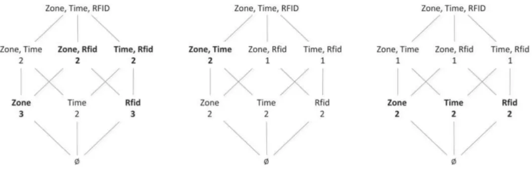
Example 12. Consider the set Σ over p-object type ðO;SÞ fromExample 1.Fig. 4shows the non-trivial subsets X of O associated with their bXi values for i = 1, 2, 3 from left to right. Among these, the duplicate sets of c-degreeβ1(left figure),β2(middle figure) andβ3(right figure) are indicated in bold font. Here, Y = {Zone, Time} is not a duplicate set of c-degreeβ1as bY2= 2 = bY1. Similarly, Z = {Rfid} is not a duplicate set of c-degreeβ2since bZ3= 2 = bZ2.
Next we characterize the structure of Armstrong p-instances. A given p-instance satisfies a given QC cardðXÞ ≤ b ∈ Σβiif there are
not b + 1 distinct objects in world wk + 1 − ithat have matching values on X. Also, a given p-instance violates all non-implied QCs if every duplicate set X of c-degreeβiis contained by some attribute set on which bXidistinct objects in wk + 1 − iagree.
Theorem 7. Let Σ denote a set of qualitative cardinality constraints, and let (ι, Possι) denote a p-instance over ðO;SÞ with jSj ¼ k þ 1. Then (ι, Possι) is an Armstrong p-instance for Σ if and only if for all i = 1, …, k, the world wk + 1 − iis Armstrong for Σβi. That is, for all i = 1, …, k,
for all X∈dupΣ
βiðOÞ there is some Z∈agbi
Xðwkþ1−iÞ such that X ⊆ Z, and for all cardðXÞ≤b∈Σβiand for all Z ∈ agb + 1(wk + 1 − i), X ⊈ Z.
Proof. The p-instance (ι, Possι) is Armstrong for Σ if and only if for all i = 1, …, k, for all QCs (φ, βi), it holds that ⊨ðι;PossιÞðφ;βiÞ iff
Σ⊨ (φ, βi). However, ⊨ðι;PossιÞðφ;βiÞ iff ⊨wkþ1−iφ, and Σ ⊨ (φ, βi) iff Σβi⊨φ. Therefore, the p-instance (ι, Possι) is Armstrong for Σ if
and only if for all i = 1, …, k, wk + 1 − iis Armstrong for Σβi. The second statement follows from the known result that a world w is
Armstrong for a set Σ of cardinality constraints if and only if for all X ∈ dupΣ(O) there is some Z ∈ agbXðwÞ such that X ⊆ Z, and for all card(X) ≤ b ∈ Σ and for all Z ∈ agb + 1(wk + 1 − i), X ⊈ Z[20,33]. □
Example 13. Consider the p-instanceι fromFig. 1and the set Σ of QCs fromExample 1.Examples 11 and 12show thatι satisfies the con-ditions ofTheorem 7, and is therefore a finite Armstrong p-instance for Σ.
5.3. Computational characterization
We now applyTheorem 7to compute Armstrong p-sketches for any given QC set over any given p-object type. It follows that Armstrong p-sketches always exist, even though finite Armstrong p-instances may not. While the problem of finding an Armstrong p-sketch is precisely exponential in the size of the given constraints we show that the size of our output Armstrong p-sketch is always bounded by the product of the number of the given constraints and the size of a minimum-sized Armstrong p-sketch. Finally, we show that there are Armstrong p-sketches whose size is logarithmic in the size of the given constraints. We recommend using both representations: i) the set Σ which explicitly lists the qualitative cardinality constraints, and ii) an Armstrong p-sketch for Σ.
For a given QC set Σ over a given p-object type ðO;SÞ and jSj ¼ k þ 1, we visualize Σ by computing an Armstrong p-sketch ς for Σ. If finite Armstrong p-instances exist for Σ, then we may compute one in the form of a p-expansion of ς.Theorem 7provides us with a strategy to compute an Armstrong p-sketch for Σ. The main complexity of this strategy goes into the computation of duplicate sets and their associated cardinalities. Conceptually, we could proceed in three stages. First, we compute for all i = 1, …, k and for all non-trivial X ⊂ O, bXiby starting with ∞ and setting bXito b whenever there is some cardðYÞ≤ b ∈ Σβisuch that Y ⊆ X and b b bX
i. Secondly, for all i = 1, …, k and starting with all non-trivial subsets X as the set of duplicate sets of c-degreeβi, we remove X whenever bXi= 1 or there is some A ∈ O − X such that bXAi = bXi.Algorithm 3calls this procedure in the loop at lines 1–3, which computes an Armstrong p-sketch for a given QC set Σ over some given p-object type ðO;SÞ. We now outline the remaining steps ofAlgorithm 3.
Algorithm 3computes objects over O∗for each duplicate set X of c-degreeβi, starting from i = k down to 1. Before moving on to another duplicate set of c-degreeβi, the algorithm processes all occurrences of X as a duplicate set of c-degreeβl≥ βi(lines 8–9), introducing an objectωr(lines 10–18) with p-degreeαk + 1 − l(line 16) and cardinality bXl − b (line 17) where b is the cardinality of the duplicate set X already processed in the previous steps (line 19). Line 23 marks X as processed to exclude it from repeated computations in the future (line 6).
For a set S let |S| denote the number of elements in S. An Armstrong p-sketch for Σ is said to be minimum-sized if there is no Armstrong p-sketch for Σ with fewer objects.
Theorem 8. Letςmindenote a minimum-sized Armstrong p-sketch for Σ.Algorithm 3computes an Armstrong p-sketchςcfor Σ such that |ςc| ≤ |ςmin| × |Σ|.
Proof. The soundness ofAlgorithm 3follows fromTheorem 7: every p-expansion of the Armstrong p-sketch computed by Algorithm 3meets the conditions inTheorem 7by construction. The upper bound on the size of the Armstrong p-sketchςccomputed byAlgorithm 3follows from a series of arguments. Firstly, the number of objects inςcequals the number of duplicate sets of c-degree βifor i = 1, …, k. Secondly, for each duplicate set of c-degreeβithere is some (card(Y) ≤ b,βj) ∈ Σ such that Y ⊆ X and j ≤ i. Thirdly, different duplicate sets X;Z ∈ dupΣ
βiðOÞ that both derive their cardinalities bX
i = bZi = b from the same (card(Y) ≤ b,βj) ∈ Σ must have different objects with p-degreeαk + 1 − iin every Armstrong p-sketch. Finally, the number of objects in any Armstrong p-sketchς equals the number of objects in its largest “world” wk. We therefore get the following:
jςcj ¼ Xk i¼1 X X∈dup∑β ið ÞO 1 ≤ Xk i¼1 ∑ðσ;βjÞ∈∑;j ≤ i ∑X∈dup∑βiðσ;β jÞ 1 ) * ) * ≤ Xk i¼1 ∑ðσ;βjÞ∈∑;j ≤ i w min kþ1−i + + +− + + +w min kþ1−i−1 + + + + + + , -, -≤ j∑j 0 jwmink j ¼ j∑j 0 jςminj
which shows the upper bound. □
Algorithm 3. Armstrong p-sketch
Note thatTheorem 8shows that qualitative cardinality constraints enjoy Armstrong sketches, that is, for every given p-object type and every given QC set Σ over this p-object type there is an Armstrong p-sketch for Σ.
We show next that the computational problem of finding an Armstrong p-sketch for Σ is precisely exponential in the size of Σ. That is, an Armstrong p-sketch for Σ can be found in time at most exponential in the size of Σ, and there are QC sets Σ such that every Armstrong p-sketch for Σ requires a number of objects that is exponential in the size of Σ.
Theorem 9. Finding an Armstrong p-sketch is precisely exponential in the size of the given set Σ of qualitative cardinality constraints. Proof. Algorithm 3computes an Armstrong p-sketch for Σ in time at most exponential in its size. Some QC sets Σ have only Armstrong p-sketches with exponentially many objects in the size of Σ. For O = {A1, …, A2n}, S ¼ fα1;α2g and Σ = {(card(A1, A2) ≤ 1,β1), …, (card(A2n − 1, A2n) ≤ 1,β1)} with size 2 ⋅ n, dupΣβ1ðOÞ consists of the 2nduplicate sets ∪j = 1n Xjwhere Xj∈ {A2j − 1, A2j}.
We also show that there other extreme cases where there are Armstrong p-sketches for QC sets Σ′ that only require a size loga-rithmic in that of Σ′.
Theorem 10. There are sets Σ′ of qualitative cardinality constraints for which there are Armstrong p-sketches whose size is logarithmic in that of Σ′.
Proof. Such a set Σ′ is given by the following 2nQCs: for all i = 1, …, n, for all X = ∪i = 1n Xiwhere Xi∈ {A2i − 1, A2i}, (card(X) ≤ 1,β1). Then the size of Σ′ is n 0 2n∈ Oð2nÞ and there is no equivalent set for Σ′ of smaller size. Furthermore, dup
Σβ1ðOÞ consists of the n sets O
− {A2i − 1, A2i} for i = 1, …, n. Thus,Algorithm 3computes an Armstrong p-sketch for Σ′ whose number of objects is in OðnÞ. □ Due toTheorems 9 and 10we recommend the use of both abstract constraint sets and their Armstrong p-sketches. Indeed, the con-straint sets enable design teams to identify concon-straints that they currently incorrectly perceive as semantically meaningful; and the Armstrong p-sketches enable design teams to identify constraints that they currently incorrectly perceive as semantically meaningless.
Our final result characterizes the situations in which finite Armstrong p-instances exist, and that the problem of deciding whether there is a finite Armstrong p-instance for a given QC set can be decided efficiently.
Theorem 11. Let Σ be a set of QCs over some given p-object type ðO;SÞ. Then there is a finite Armstrong p-instance for Σ if and only if for all A ∈ O there is some b ∈ ℕ such that Σ implies (card(A) ≤ b,β1). It can therefore be decided in time OðjOj 1 jjΣjjÞ whether there is a finite Armstrong p-instance for Σ.
Proof. If it is true that for all A ∈ O there is some b ∈ ℕ such that Σ implies (card(A) ≤ b,β1), then bXi
b ∞ for all non-empty X ⊂ O. Hence, every p-expansion of an Armstrong p-sketch thatAlgorithm 3computes is finite. Vice versa, suppose there is some A ∈ O such that Σ does not imply (card(A) ≤ b,β1) for any b ∈ ℕ. Consequently, there is some duplicate set X of c-degreeβ1and A ∈ X such that bX1= ∞. Theorem 7shows that every Armstrong p-instance for Σ must contain infinitely many objects that agree on X. The condition that for all A ∈ O there is some b ∈ ℕ such that Σ implies (card(A) ≤ b,β1) can be verified in time OðjOj 1 jjΣjjÞ. □
6. Implementation
We have implementedAlgorithm 3within a prototype system. The system enables users to enter a p-object type and a finite set of p-cardinality constraints over this type, and computes an Armstrong p-sketch for the constraint set. We illustrate the basic function-ality of our system by some examples.
6.1. Running example
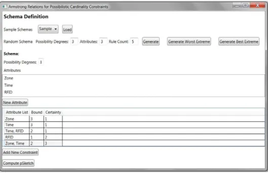
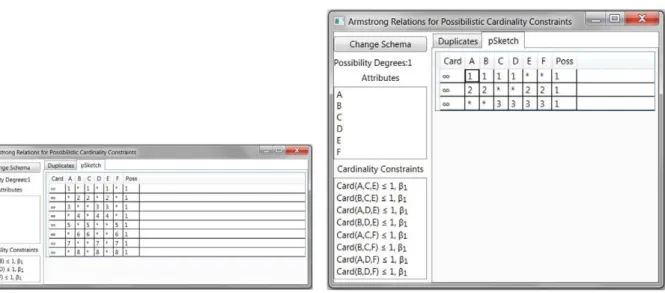
We begin with some screenshots that show how the instance fromExample 10is processed by our system. The left ofFig. 5shows the input interface where the p-object type and input constraint set ofExample 10have been entered. The figure also shows that our system can randomly generate input that complies with any user specification of the following parameters: number of p-degrees, number of attributes, and number of cardinality constraints.
The left ofFig. 6shows the Armstrong p-sketch for the input constraint set ofExample 10as computed by our prototype system. Note that only integer values are used as domain values and that these can be interpreted as indices for actual domain values, where different indices represent different domain values. Similarly, the integer i in the column Poss represents the p-degreeαi. Observe that the p-sketch shown in the left ofFig. 6is isomorphic to the p-sketch shown inTable 4.
As an explanation of the p-sketch, our prototype system can also show the duplicate sets it computes as part ofAlgorithm 3. The right ofFig. 6shows the duplicate sets for the input constraint set ofExample 10. The system shows for each attribute subset X and for each c-degreeβi, the minimum upper bound bXithat can be inferred from the input constraints. The system indicates by T that a given attribute subset is a duplicate set of c-degreeβi.
6.2. Extreme cases
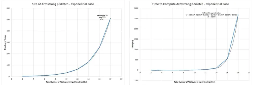
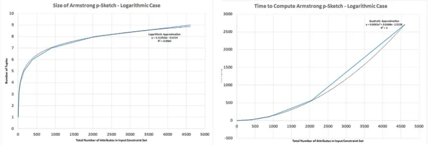
Fig. 5shows that our system can automatically generate instances of the extreme cases of p-cardinality constraints reported in Theorems 9 and 10, for any given even number of attributes. The left ofFig. 7shows the output for the case n = 3 ofTheorem 9,