Blind regression : nonparametric regression for latent variable models via collaborative filtering

(1)

Blind Regression: Nonparametric Regression for

Latent Variable Models via Collaborative Filtering

by

Dogyoon Song

Submitted to the Department of Electrical Engineering and Computer

Science

in partial fulfillment of the requirements for the degree of

Master of Science in Electrical Engineering and Computer Science

at the

MASSACHUSETTS INSTITUTE OF TECHNOLOGY

June 2016

c

○ Massachusetts Institute of Technology 2016. All rights reserved.

Author . . . .

Department of Electrical Engineering and Computer Science

May 20, 2016

Certified by . . . .

Devavrat Shah

Professor

Thesis Supervisor

Accepted by . . . .

Leslie A. Kolodziejski

Chair, Department Committee on Graduate Students

(2)

(3)

Blind Regression: Nonparametric Regression for Latent

Variable Models via Collaborative Filtering

by

Dogyoon Song

Submitted to the Department of Electrical Engineering and Computer Science on May 20, 2016, in partial fulfillment of the

requirements for the degree of

Master of Science in Electrical Engineering and Computer Science

Abstract

Recommender systems are tools that provide suggestions for items that are most likely to be of interest to a particular user; they are central to various decision making processes so that recommender systems have become ubiquitous. We introduce blind regression, a framework motivated by matrix completion for recommender systems: given 𝑚 users, 𝑛 items, and a subset of user-item ratings, the goal is to predict the unobserved ratings given the data, i.e., to complete the partially observed matrix. We posit that user 𝑢 and movie 𝑖 have features 𝑥1(𝑢) and 𝑥2(𝑖) respectively, and

their corresponding rating 𝑦(𝑢, 𝑖) is a noisy measurement of 𝑓 (𝑥1(𝑢), 𝑥2(𝑖)) for some

unknown function 𝑓 . In contrast to classical regression, the features 𝑥 = (𝑥1(𝑢), 𝑥2(𝑖))

are not observed (latent), making it challenging to apply standard regression methods. We suggest a two-step procedure to overcome this challenge: 1) estimate distance for latent variables, and then 2) apply nonparametric regression. Applying this frame-work to matrix completion, we provide a prediction algorithm that is consistent for all Lipschitz functions. In fact, the analysis naturally leads to a variant of collaborative filtering, shedding insight into the widespread success of collaborative filtering. As-suming each entry is revealed independently with 𝑝 = max(𝑚−1+𝛿, 𝑛−1/2+𝛿) for 𝛿 > 0, we prove that the expected fraction of our estimates with error greater than 𝜖 is less than 𝛾2/𝜖2, plus a polynomially decaying term, where 𝛾2 is the variance of the noise. Experiments with the MovieLens and Netflix datasets suggest that our algorithm provides principled improvements over basic collaborative filtering and is competitive with matrix factorization methods. The algorithm and analysis naturally extend to higher order tensor completion by simply flattening the tensor into a matrix. We show that our simple and principled approach is competitive with respect to state-of-art tensor completion algorithms when applied to image inpainting data. Lastly, we conclude this thesis by proposing various related directions for future research. Thesis Supervisor: Devavrat Shah

(4)

(5)

Acknowledgments

I would like to express my gratitude to my thesis supervisor, Devavrat Shah, for all his guidance and encouragement over the last two years.

I would also like to thank Christina Lee and Yihua Li for helpful discussions on related subjects.

Lastly, I would like to thank my parents, whom I owe everything for their uncon-ditional love.

This research was supported in part by a Samsung Scholarship, an MIT EECS Advanced Television & Signal Processing Fellowship, and a Siebel Scholarship.

(6)

(7)

List of Figures

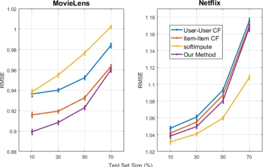
6-1 Performance of algorithms on Netflix and MovieLens data set with 95% confidence interval. 𝜆 values used by our algorithm are 2.8 (10%), 2.3 (30%), 1.7 (50%), 1 (70%) for MovieLens, and 1.8 (10%), 1.7 (30%), 1.6 (50%), 1.5 (70%) for Netflix. . . 67 6-2 Performance comparison between different tensor completion algorithms

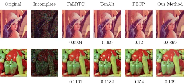
based on RSE vs testing set size. For our method, we set overlap pa-rameter 𝛽 to 2. . . 68 6-3 Recovery results for Lenna, Pepper and Facade images with 70% of

missing entries. RSE is reported under the recovery images. . . 69 6-4 Risk𝜖 achieved on MovieLens data set (10% evaluation). . . 70

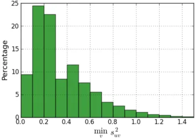
6-5 Effect of 𝜆 on RMSE from MovieLens data set (10% evaluation). . . . 70 6-6 Distribution of minimum sample variance (𝛽 = 5). . . 71 6-7 Variation of squared error across min𝑣𝑠2𝑢𝑣 buckets (𝛽 = 5). The red

line plots the median, while the box shows the 25𝑡ℎ_{and 75}𝑡ℎ_percentile,

and end of dashed lines extends to the most extreme data point within 1.5 interquartile range of the upper quartile. . . 72

(12)

(13)

Chapter 1 Introduction

1.1 Background

Recommender systems have become ubiquitous in our lives. They help us filter a vast amount of information we encounter into smaller selections of likable items customized to the users’ tastes. Amazon recommends items to customers; Netflix recommends movies to users; and LinkedIn recommends job positions to users or candidate profiles to recruiters.

There have been many studies on recommender systems, which were fueled by the Netflix Prize competition that began in October 2006 [5,6,7]. Because of the compe-tition, the research community was able to gain access to large-scale data consisting of 100 million movie ratings, and a huge group of researchers were attracted to attack the problem. The competition has encouraged rapid development in techniques to improve prediction accuracy. As a result, much progress has been made in the field of collaborative filtering.

One natural approach for recommendation is to use auxiliary/exogenous content information about the users or items. For example, the information on the director, the lineup of actors, genre, or the language can help us figure out whether two movies are similar or not. Likewise, information including age, geographic location, and academic background reveals some characteristics of a user. Recommendations based on such content-specific data is called content filtering [4, 8, 44]. With quantitative

(14)

content features, this setting becomes that of traditional regression problems.

However, in practice, recommendations are often made via a technique called col-laborative filtering (CF), which provides recommendations in a content-agnostic way by exploiting patterns to determine similarity between users or items. The use of such techniques is partly because the exogenous content information (or its quantitative representation) is usually not available. Moreover, it is known that recommender systems purely based on content generally suffer from the problems of limited content analysis and over-specialization [48].

Instead of relying on content information, collaborative filtering approaches use the rating information of other users and items in the system. For example, if two users are revealed to have similar tastes, a CF algorithm might recommend the items the first user liked to the second user (user-user CF). On the other hand, if many users agree on two items, a CF algorithm might recommend the second item to a user who likes the first (item-item CF). Collaborative filtering has been successful and used extensively for decades including Amazon’s recommendation system [32] and the Netflix Prize winning algorithm by BellKor’s Pragmatic Chaos [29].

There are two primary approaches to relate two different entities: users and items, by utilizing such similarities. They are two main branches of CF: one is the neighborhood-based mehod, and the other is the latent factor method (=model-based method). Neighborhood-based methods concentrate on similarities (or relationships) between items or between items. For example, an item-item CF models the prefer-ence of a user for an item based on the past ratings of similar items by the user. Latent factor methods comprise an alternative approach by transforming both items and users to the same (low-dimensional) latent factor space. Matrix factorization methods, such as singular value decomposition (SVD) is an example of a latent factor method [30, 41].

Although latent factor models have gained popularity because of their relatively high accuracy and theoretical elegance, neighborhood-based approaches to CF are still widely used in practice. One reason for this is that good prediction accuracy is not the sole objective for recommender systems. Other factors, for instance, recommendation

(15)

serendipity, can play an important role in the appreciation of users [21,47].

The main advantages of neighborhood-based methods are as follows. They are intuitive and simple to implement (simplicity). They can provide intuitive explana-tions for the reasons recommendaexplana-tions work (justifiability). Unlike most model-based systems, they require less or no costs of training phases, which need to be carried at frequent intervals in large commercial applications; meanwhile, storing nearest neighbors requires very little memory (efficiency). In addition, a neighborhood-based approach is little affected by the constant addition of new data (stability). That is, once item similarities have been computed, an item-based system can readily provide immediate recommendations to a newly entered user based on her feedback. This property makes it desirable for an online recommendation setting [41].

1.2 Related Work

The term collaborative filtering was coined in [19]. Collaborative filtering approaches can be grouped into two general classes: model and neighborhood-based methods.

Model-based CF: Model-based approaches use the stored ratings to learn a pre-dictive model. Principal characteristics of users and items are captured by a set of model parameters, learned from a training dataset, and used to predict ratings on new items. There have been numerous model-based approaches toward the task of recommendation, which include Bayesian Clustering [11], Latent Dirichlet Allocation [9], Maximum Entropy [54], Boltzmann Machines [46], Support Vector Machines [20], and Singular Value Decomposition [50, 43, 28, 51].

Low-rank Matrix Factorization: In the recent years, there has been excit-ing theoretical development in the context of matrix-factorization-based approaches. Since any matrix can be factorized, its entries can be described by a function with the form 𝑓 (𝑥1, 𝑥2) = 𝑥𝑇1𝑑𝑖𝑎𝑔(𝜎)𝑥2, and the goal of factorization is to recover the

la-tent features for each row and column. [50] was one of the earlier works to suggest the use of low-rank matrix approximation, observing that a low-rank matrix has a

(16)

comparatively small number of free parameters. Subsequently, statistically efficient approaches were suggested using optimization based estimators, proving that ma-trix factorization can fill in the missing entries with sample complexity as low as 𝑟𝑛 log 𝑛, where 𝑟 is the rank of the matrix [15, 25, 45, 40, 23]. Also, there has been an exciting line of ongoing work to make the resulting algorithms faster and scalable [17, 14,31, 49, 34,38].

These approaches are based on the structural assumption that the underlying ma-trix is low-rank and the mama-trix entries are reasonably “incoherent”. Unfortunately, the low-rank assumption may not hold in practice. The recent work [18] makes pre-cisely this observation, showing that a simple non-linear, monotonic transformation of a low-rank matrix could easily produce an effectively high-rank matrix, despite few free model parameters. They provide an algorithm and analysis specific to the form of their model, which achieves sample complexity of 𝑂((𝑚𝑛)2/3). However, their algorithm only applies to functions 𝑓 which are a nonlinear monotonic transformation of the inner product of the latent features. The limitations of these approaches lie in the restrictive assumptions of the model.

Neighborhood-based CF: In neighborhood-based (also called memory-based) collaborative filtering, the stored user-item ratings are directly used to predict ratings for new pairs of user-item. This prediction can be done in two ways: user-based or item-based. User-based systems, such as Ringo [48], GroupLens [27], and Bellcore video [22], evaluate the preference of a target user for items by using the ratings for the items by other users (neighbors) who have similar preference patterns.

There are two main paradigms in neighborhood-based collaborative filtering: the user-user paradigm and the item-item paradigm. To recommend items to a user in the user-user paradigm, one first looks for similar users, and then recommends items liked by those similar users. In the item-item paradigm, in contrast, items similar to those liked by the user are found and subsequently recommended. Much empirical evidence exists that the item-item paradigm performs well in many cases [47, 32,

(17)

recent works, Latent mixture models have been introduced to explain the collaborative filtering algorithm as well as the empirically observed superior performance of item-item paradigms, c.f. [12, 13].

However, these results assume a specific parametric model, such as a mixture distribution model for preferences across users and movies. We hope that by provid-ing an analysis for collaborative filterprovid-ing within our broader nonparametric model, we can provide a more complete understanding of the potentials and limitations of collaborative filtering.

Tensor completion: A tensor is the higher-dimensional analogue of a matrix (or a vector). Therefore, it is natural to consider extending the neighborhood-based ap-proaches to the context of tensor completion; however, there is little known literature about this setting.

Tensor completion is known to be much harder than matrix completion. Ten-sors do not have a canonical decomposition such as the singular value decomposition (SVD) for a matrix, which simultaneously possesses two desirable properties: (i) it computes a rank-r decomposition, and (ii) it yields orthonormal row/column matri-ces. These properties makes obtaining a decomposition for a tensor challenging [26]. There have been recent developments in obtaining an efficient rank-1 tensor decompo-sition [1], which is effective in learning latent variable models and estimating missing data [24, 42]. In the context of learning latent variable models or mixture distri-butions, there have been developments in non-negative matrix/tensor factorizations [3,2] which go beyond SVD.

Kernel regression: The algorithm we propose in this work is inspired by the local approximation of functions by the Taylor series expansion. We would first build local estimators with observed ratings, and then combine these with appropriately chosen weights. For this reason, there is a connection to the classical setting of kernel regression, which also relies on smoothed local approximations [35, 52]. However, both the power series expansion and the kernel regression require explicit knowledge

(18)

of the geometry of feature space, which is not permitted in the setting of recommender systems. As a result, their analysis and proof techniques do not extend to our context of Blind regression, in which the features are latent; the analysis required is entirely different despite the similarity in the form of computing a convex combination of nearby datapoints.

1.3 Our Contribution

In contrast to numerous empirical attempts to obtain accurate prediction methods, we have few theoretical studies on neighborhood-based models. One objective of this thesis is to provide a general statistical framework for performing nonparametric regression over latent variable models, from which a neighborhood-based algorithm with provable performance bounds follows. We are initially motivated by the problem of matrix completion arising in the context of designing recommendation systems, but we additionally show that our framework allows for systematic extensions to higher order tensor completion as well.

In the popularized setting of Netflix, there are 𝑚 users, indexed by 𝑢 ∈ [𝑚], and 𝑛 movies, indexed by 𝑖 ∈ [𝑛]. Each user 𝑢 has a rating for each movie 𝑖, denoted as 𝑦(𝑢, 𝑖). The system observes ratings for only a small fraction of user-movie pairs. The goal is to predict ratings for the rest of the unknown user-movie pairs, i.e., to complete the partially observed 𝑚 × 𝑛 rating matrix. To be able to obtain meaningful predictions from the partially observed matrix, it is essential to impose a structure on the data.

We assume each user 𝑢 and movie 𝑖 is associated to features 𝑥1(𝑢) ∈ 𝒳1 and

𝑥2(𝑖) ∈ 𝒳2 for some compact metric spaces 𝒳1, 𝒳2. We assume that the latent features

are drawn independently from an identical distribution (IID) with respect to some Borel probability measures on 𝒳1, 𝒳2. Following the philosophy of non-parametric

(19)

rating of user 𝑢 for movie 𝑖 is given by

𝑦(𝑢, 𝑖) = 𝑓 (𝑥1(𝑢), 𝑥2(𝑖)) + 𝜂𝑢𝑖, (1.1)

where 𝜂𝑢𝑖 is some independent bounded noise. However, we refrain from any specific

modeling assumptions on 𝑓 , requiring only mild regularity conditions following the traditions of non-parametric statistics. We observe ratings for a subset of the user-movie pairs, and the goal is to use the given data to predict 𝑓 (𝑥1(𝑢), 𝑥2(𝑖)) for all

(𝑢, 𝑖) ∈ [𝑚] × [𝑛] whose rating is unknown.

In classical nonparametric regression, we observe input features 𝑥1(𝑢), 𝑥2(𝑖) along

with the rating 𝑦(𝑢, 𝑖) for each datapoint, and thus we can approximate the function 𝑓 well using local approximation techniques as long as 𝑓 satisfies mild regularity conditions. However, in our setting, we do not observe the latent features 𝑥1(𝑢), 𝑥2(𝑖),

but instead we only observe the indices (𝑢, 𝑖). Therefore, we use blind regression to refer to the challenge of performing regression with unobserved latent input variables. This paper addresses the question, does there exist a meaningful prediction algorithm for general nonparametric regression when the input features are unobserved?

Our answer is “yes.” In spite of the minimal assumptions of our model, we provide a consistent matrix completion algorithm with finite sample error bounds as well. Furthermore, as a coincidental by-product, we find that our framework provides an explanation for the mystery of “why collaborative filtering algorithms work well in practice.”

As the main technical result, we show that the user-user nearest neighbor variant of collaborative filtering method with our similarity metric yields a consistent estimator for any Lipschitz function as long as we observe max(𝑚−1+𝛿, 𝑛−1/2+𝛿) fraction of the matrix with 𝛿 > 0. In the process, we obtain finite sample error bounds, whose details are stated in Theorem 1. We compared the Gaussian kernel variant of our algorithm to classic collaborative filtering algorithms and a matrix factorization based approach (softImpute) on predicting user-movie ratings for the Netflix and MovieLens datasets. Experiments suggest that our method improves over existing collaborative

(20)

filtering methods, and sometimes outperforms matrix-factorization-based approaches depending on the dataset.

There are two conceptual parts to our algorithm. First, we derive an estimate of 𝑓 (𝑥1(𝑢), 𝑥2(𝑖)) for an unobserved index pair (𝑢, 𝑖) by using linear approximation

of 𝑓 pivoted at (𝑥1(𝑢′), 𝑥2(𝑖′)). By Taylor’s theorem, this estimates the unknwon

𝑓 (𝑥1(𝑢), 𝑥2(𝑖)) quite well as long as 𝑥1(𝑢′) is close to 𝑥1(𝑢) or 𝑥2(𝑖′) is close to 𝑥2(𝑖).

However, since the latent features are not observed, we need a method to approxi-mate the distance in the latent space. The second observation we make is that under our mild Lipschitz conditions, the similarity metrics commonly used in collaborative filtering heuristics correspond to an estimate of distances in the latent space. In par-ticular, we use the sample variance of the differences between observations between a pair of users to capture distances between two users in this thesis. Formally speaking, we cannot guarantee that if the sample variance is small, the distance in the latent space is small, yet we show in our analysis that there is a direct relation between the sample variance and the estimation error.

To analyze the performance of our algorithm, we make minimal model assumptions just like any such work in non-parametric statistics. Let the latent features be drawn independently from an identical distribution (IID) over a compact metric spaces; the function 𝑓 is Lipschitz with respect to the latent space metrics; entries are observed independently with some probability 𝑝; and the additive noise in observations is bounded and independently distributed with zero mean.

In addition, there is no reason to limit ourselves to bivariate functions 𝑓 in (1.1). The equivalent extension of the bivariate latent variable model to multivariate latent models is to extend from matrices to higher order tensors. The algorithm and analysis that we provide for matrix completion also extends to higher order tensor completion, due to the flexible and generic assumptions of our model.

The algorithm discussed above, as well as its analysis, naturally extends beyond matrices, to completing higher order tensors. In Section 4.2, we show that the tensor completion problem can be reduced to matrix completion, and thus we have a con-sistent estimator for tensor completion under similar model assumptions. We show

(21)

in experiments that our method is competitive with respect to state of the art tensor completion methods when applied to the the image inpainting problem. Our esti-mator is naively simple to implement, and its analysis sidesteps the complications of non-unique tensor decompositions. The ability to seamlessly extend beyond matri-ces to higher order tensors suggests the general applicability and value of the blind regression framework.

1.4 Organization of Thesis

In Chapter 2 of this thesis, we propose a novel nonparametric framework to make predictions without knowledge on the latent function and feature representations. The framework comprises two steps: 1) estimating the distance between unknown feature representations, and 2) running nonparametric kernel regression. Unlike low-rank matrix factorization techniques, this framework does not require strict structural assumptions. Meanwhile, the framework may not need the explicit feature represen-tations of the input, but only their identifiers. This property justifies the name ’blind’ regression and differentiates our framework from classical nonparametric regression.

In Chapter 3, we suggest a recommendation algorithm based on the suggested framework. It is essentially a neighborhood-based algorithm, motivated by the Tay-lor series expansion and the idea of boosting, which is a machine learning technique. The suggested algorithm is simple to implement, widely applicable due to its non-parametric nature, and fairly competitive in terms of its prediction accuracy.

In Chapter 4, we present our main technical results for the proposed algorithm. To the best of our knowledge, this analysis provides the first provable performance bounds on the sample complexity and prediction accuracy of neighborhood-based methods. Our algorithm is proven to be a consistent estimation algorithm as the size of the matrix grows infinitely large. In Section 4.2, the analysis extends to the tensor completion setting via flattening. In addition, the trade-off of averaging multiple estimators is briefly discussed in Section 4.3 under a set of simplifying assumptions.

(22)

section of this chapter contains a key lemma used in the proof of the theorem, and auxiliary lemmas if necessary. The proof of the lemmas are based on various concen-tration inequality techniques, whose details can be found in the Appendix.

In Chapter 6, we present the performance of our algorithm with experiments on real world datasets. First of all, we show our algorithm outperforms other neighbor-based collaborative filtering algorithms on MovieLens and Netflix datasets. Also, its performance is comparable to a matrix factorization method (SoftImpute). Next, we apply our algorithm for image reconstruction via tensor flattening. Despite its simplicity, our algorithm performs nearly as good as the best tensor completion algo-rithms reported.

In Chapter 7 we summarize all the pieces and discuss some directions for future work.

(23)

Chapter 2 Blind Regression

This chapter covers the introduction to our novel framework of blind regression. Re-gression is a statistical process for estimating relationships among variables, which help to understand how dependent variable varies as one or more independent vari-ables changes. Regression includes many techniques, and is widely used for prediction. However, geometric information on the feature space is essential for all of these tech-niques, whereas it is not available for the class of problems we are interested in. In this chapter, we will briefly review regression, with an emphasis on kernel regression, a non-parametric technique. Then, we will describe the blind regression framework, pointing out its connection to the traditional regression as well as its unique features.

2.1 Traditional Regression

2.1.1 Regression Regime

Regression is a statistcal process for estimating relationships among variables. More specifically, the aim of regression analysis is to describe the value of a dependent variable in terms of other variables. This objective is achieved by estimating a target function of independent variables, called regression function. In many cases, it is also of interest to characterize the variation of dependent variable around the regression function, which can measure the descriptive power of the regression function.

(24)

Regression analysis is widely used for prediction and forecasting, and thus has connection to the field of machine learning. Consider the following situation, which is familiar in supervised learning context: we are given a traning dataset consisting of 𝑁 labeled data points {(𝑥𝑖, 𝑦𝑖)}𝑁𝑖=1. Our task is to estimate the relationship between

the feature 𝑥𝑖 and the response 𝑦𝑖, or to learn the structure concealed in the data, in

order to make a prediction ˆ𝑦 when given a new input 𝑥.

There are many techniques developed for regression analysis. Some methods, such as linear regression and ordinary least squares estimation, are parametric, in which the regression function is defined in terms of a finite number of unknown parameters to be estimated from the data. On the other hand, nonparametric regression techniques allow the regression function to lie in a more general class of functions, which may possibly constitute an infinite-dimensional space of functions.

Parametric regression models assume a specific form of the underlying function y = 𝑓𝛽(x) where the model involves the following variables: the independent variables

x ∈ R𝑑

; the dependent variable y ∈ R; and the unknown parameters 𝛽. For example, a linear regression model can be written as

𝑌 = ⎡ ⎢ ⎢ ⎢ ⎢ ⎢ ⎢ ⎣ 𝑦1 𝑦2 .. . 𝑦𝑛 ⎤ ⎥ ⎥ ⎥ ⎥ ⎥ ⎥ ⎦ = ⎡ ⎢ ⎢ ⎢ ⎢ ⎢ ⎢ ⎣ 1 𝑥1 1 𝑥2 .. . ... 1 𝑥𝑛 ⎤ ⎥ ⎥ ⎥ ⎥ ⎥ ⎥ ⎦ ⎡ ⎣ 𝛽0 𝛽1 ⎤ ⎦+ 𝜖 = 𝑋𝛽 + 𝜖,

and the objective is to estimate the parameter 𝛽 = (𝛽0, 𝛽1)𝑇 ∈ R𝑑+1 from the data.

Sometimes, the matrix 𝑋, a stack of independent variable instances [︁

1 𝑥𝑖

]︁

, is called a design matrix. This kind of structural assumption simplifies the problem and makes the parametric models easier to implement and analyze.

One of the most famous and standard approaches to parametric regression is the method of least squares. It attempts to minimize the mean squared error in the dependent variables, or the sum of squared residuals ∑︀𝑁

𝑖=1(𝑦𝑖− 𝑥𝑖𝛽) 2

, assuming there are zero or negligible errors in the independent variables. It has closed-form expressions for ˆ𝛽 = (𝑋𝑇𝑋)−1𝑋𝑇𝑌 and a nice geometric interpretation. The least

(25)

square solution ˆy(x) = x ˆ𝛽 is a Euclidean projection of 𝑦 onto the subspace spanned by 𝑋.

Although parametric approaches are efficient, making incorrect structural assump-tions may result in a poor estimator. For example, estimating a trigonometric func-tion with polynomial bases will require an unnecessarily large number of parameters. Moreover, an attempt to estimate a quadratic function with a linear model will not be productive. Sometimes, machine learning practitioners deal with this problem with model selection and regularization techniques.

There is an alternative approach to overcome the rigidity of parametric regression, which is commonly referred to as nonparametric regression. This is a generic term for methods which do not make a priori structural assumptions for the underlying function. Typical examples include kernel regression and spline interpolation, which allow the data to decide which function fits them the best via local approximation. Abandoning such restrictions imposed by a parametric model allows more general-ity for this approach. However, nonparametric methods are computationally more expensive compared to parametric models.

2.1.2 Kernel Regression

There are several approaches to the nonparametric regression. Some of the most pop-ular methods are based on local function smoothing, using kernel functions, spline functions, and wavelets. Each of these techniques has its own strengths and weak-nesses. Among various nonparametric estimators, kernel estimators have the advan-tage of being intuitive, and are simple to analyze.

In any nonparametric regression, the objective is to find an estimator ˆ𝑓 (𝑋) for the conditional expectation E [𝑌 |𝑋] of a dependent variable 𝑌 relative to a given independent variable 𝑋. Kernel regression is a technique to estimate this conditional expectation as a locally weighted average, using kernel as a weighting function.

(26)

esti-mator: ˆ 𝑓𝜆(𝑥) = ∑︀𝑛 𝑖=1𝐾𝜆(𝑥, 𝑥𝑖)𝑦𝑖 ∑︀𝑛 𝑖=1𝐾𝜆(𝑥, 𝑥𝑖) ,

where 𝐾 is a kernel with a bandwidth ℎ. A kernel determines the intensity of influence one point can exert on other points, while the bandwidth ℎ controls how fast the effect decays in space.

This estimator is known to be consistent when certain technical conditions on the kernel 𝐾 and the bandwidth 𝜆 are satisifed. For the rest of this thesis, we will exclusively consider the Gaussian kernel (also known as the heat kernel):

𝐾𝜆(𝑥, 𝑥𝑖) = 𝑒−𝜆(𝑥−𝑥𝑖)

2

.

2.2 Blind Regression

We are interested in a certain class of problems, for which each instance of indepen-dent variable 𝑥𝑖 is distinguishable by identities, but there is no meaningful feature

representation. For example, Amazon can distinguish one customer from another from their customer IDs, but their IDs are arbitrary and do not represent their char-acteristics. In addition, they do not provide any clue on the distance between two users. This makes the traditional regression approach impossible because all the above approaches rely on the geometry of feature representations. In fact, having such a void representation is quite easily observed in real-world data applications.

This challenge mainly arises from the fact that we do not have a metric to measure distance between any two datapoints without having meaningful feature representa-tions. Therefore, we suggest to learn geometry of a latent representation of data from the data themselves. In some applications, such as recommender systems, the notion of similarity between users or between items is already widely used. We propose to unify such heuristic approaches in language of a pseudo-metric in the latent space and kernel regression.

The term ‘blind regression’ refers to this two-step procedure: 1) estimate the distance between data points, using heuristics if applicable; and 2) make prediction

(27)

based on a kernel regression estimator. One benefit of this framework is that we can adopt techniques for kernel regression to analyze estimators that can be parsed via lens of blind regression.

In the following chapters, we apply this framework to build and analyze neighbor-based algorithms for matrix completion.

(28)

(29)

Chapter 3 Application to Matrix Completion

In this chapter, we apply the blind regression framework to the matrix completion problem. We will describe the problem, and our modeling assumptions to obtain provable guarantees in the following chapters. Then we will describe our collaborative filtering algorithm, with two variants which will be analyzed in subsequent chapters. We will also provide some intuition behind the algorithm.

3.1 Model and Notation

3.1.1 Motivation

Our work is motivated by the problem of matrix completion arising in the context of designing recommendation systems. In the popularized setting of the Neflix Chal-lenge, there are 𝑚 users, indexed by 𝑢 ∈ [𝑚], and 𝑛 movies, indexed by 𝑖 ∈ [𝑛]. Each user 𝑢 has a rating for each movie 𝑖, denoted as 𝑅(𝑢, 𝑖). The system observes ratings for only a small fraction of user-movie pairs. The goal is to predict ratings for the rest of the unknown user-movie pairs, i.e., to complete the partially observed 𝑚 × 𝑛 rating matrix. To be able to obtain meaningful predictions from the partially observed matrix, it is essential to impose a structure on the data.

(30)

3.1.2 Model and Assumptions

Model. We assume the following data generation process: each user 𝑢 and movie 𝑖 is associated to feature representations 𝑥1(𝑢) ∈ 𝒳1 and 𝑥2(𝑖) ∈ 𝒳2 for some metric

spaces 𝒳1, 𝒳2. The rating of user 𝑢 for movie 𝑖 is given by

𝑅(𝑢, 𝑖) = 𝑓 (𝑥1(𝑢), 𝑥2(𝑖)) ,

for some function 𝑓 : 𝒳1× 𝒳2 → R.

We observe ratings for 𝑁 ≪ 𝑚×𝑛 user-movie pairs, denoted as 𝒟 ={︀(𝑢𝑘_{, 𝑖}𝑘_{, 𝑅}𝑘₎}︀𝑁

𝑘=1,

where (𝑢𝑘_{, 𝑖}𝑘_{, 𝑅}𝑘_{) ∈ [𝑚] × [𝑛] × R. Also, we assume that the measurements are noisy:}

𝐴(𝑢, 𝑖) = 𝑅(𝑢, 𝑖) + 𝜂(𝑢, 𝑖), (3.1)

for (𝑢, 𝑖, 𝑅) ∈ 𝒟 with noise 𝜂(𝑢, 𝑖). The goal is to use the data 𝒟 to predict 𝑅(𝑢, 𝑖) for all (𝑢, 𝑖) ∈ [𝑚] × [𝑛] whose rating is unknown.

For brevity, this can be summarized as follows in terms of matrices: we are given an incomplete matrix 𝐴 ∈ R𝑚×𝑛 _{generated by}

𝐴 = 𝑀 ∘ (𝑅 + 𝐸) .

where ∘ is the Hadamard product (= entrywise multiplication) and

∙ The mask matrix 𝑀 takes either 1 or ∞

𝑀 (𝑢, 𝑖) = ⎧ ⎪ ⎨ ⎪ ⎩ 1 if (𝑢, 𝑖, 𝑅(𝑢, 𝑖)) ∈ 𝒟, ∞, otherwise.

∙ Each entry of the noise matrix 𝐸 represents i.i.d. additive noise

(31)

Assumptions. We shall make the following assumptions on regularity of the latent spaces 𝒳1, 𝒳2 (assumptions 1 and 2), the latent function 𝑓 (assumption 3), the noise

𝜂 (assumption 4), and the dataset 𝒟 (assumption 5).

1. 𝒳1 and 𝒳2 are compact metric (therefore totally bounded, and hence bounded)

spaces endowed with metrics 𝑑1 and 𝑑2 respectively:

𝑑1(𝑥1, 𝑥′1) ≤ 𝐵, ∀𝑥1, 𝑥′1 ∈ 𝒳1,

𝑑2(𝑥2, 𝑥′2) ≤ 𝐵, ∀𝑥2, 𝑥′2 ∈ 𝒳2.

2. Let 𝑃1 and 𝑃2 be Borel probability measures on (𝒳1, 𝑇1) and (𝒳2, 𝑇2),

respec-tively, where 𝑇𝑖 denotes the Borel 𝜎-algebra of 𝒳𝑖 generated by the metric 𝑑𝑖

above. We shall assume that the latent features of each user 𝑢 and movie 𝑖, 𝑥1(𝑢) and 𝑥2(𝑖), are drawn i.i.d. from the distribution given by 𝑃1 and 𝑃2

respectively.

3. The latent function 𝑓 : 𝒳1× 𝒳2 → R is 𝐿-Lipschitz with respect to ∞-product

metric (see Definition 3 in Appendix A.1) of 𝑑1 and 𝑑2:

|𝑓 (𝑥1, 𝑥2) − 𝑓 (𝑥′1, 𝑥 ′

2)| ≤ 𝐿 (𝑑1(𝑥1, 𝑥′1) ∨ 𝑑2(𝑥2, 𝑥′2)) , ∀𝑥1, 𝑥′1 ∈ 𝒳1, ∀𝑥2, 𝑥′2 ∈ 𝒳2.

4. The additive noise for all data points are independent and bounded with zero mean and variance 𝛾2_{: for all 𝑢 ∈ [𝑛}

1], 𝑖 ∈ [𝑛2],

𝜂(𝑢, 𝑖) ∈ [−𝐵𝜂, 𝐵𝜂], E[𝜂(𝑢, 𝑖)] = 0, Var[𝜂(𝑢, 𝑖)] = 𝛾2.

5. Rating of each entry is revealed (observed) with probability 𝑝, independently. In other words,

(32)

3.1.3 Notations

We introduce some notations which will be used in later sections.

Index sets: We let 𝒪𝑢 denote the set of column indices of observed entries in row

𝑢. Similarly, let 𝒪𝑖 denote the set of row indices of the observed in column 𝑖, namely,

𝒪𝑢 := {𝑖 : 𝑀 (𝑢, 𝑖) = 1},

𝒪𝑖 := {𝑢 : 𝑀 (𝑢, 𝑖) = 1}.

For rows 𝑣 ̸= 𝑢, we define the overlap between two rows 𝑢 and 𝑣 as

𝒪𝑢𝑣 := 𝒪𝑢∩ 𝒪𝑣,

the set of column indices of commonly observed entries for the pair of rows (𝑢, 𝑣). Similarly, the overlap between two columns 𝑖 and 𝑗 (𝑗 ̸= 𝑖) is defined as

𝒪𝑖𝑗 := 𝒪𝑖∩ 𝒪𝑗.

𝛽-overlapping neighbors: Given a parameter 𝛽 ≥ 2, and (𝑢, 𝑖), define 𝛽-overlapping neighbors of 𝑢 and 𝑖 respectively as

𝒮𝛽

𝑢(𝑖) = {𝑣 𝑠.𝑡. 𝑣 ∈ 𝒪𝑖, 𝑣 ̸= 𝑢, |𝒪𝑢𝑣| ≥ 𝛽},

𝒮_𝑖𝛽(𝑢) = {𝑗 𝑠.𝑡. 𝑗 ∈ 𝒪𝑢, 𝑗 ̸= 𝑖, |𝒪𝑖𝑗| ≥ 𝛽}.

Empirical statistics: For each 𝑣 ∈ 𝒮_𝑢𝛽(𝑖), we can compute the empirical row variance between 𝑢 and 𝑣,

𝑠2_𝑢𝑣 := 1

2 |𝒪𝑢𝑣| (|𝒪𝑢𝑣| − 1)

∑︁

𝑖,𝑗∈𝒪𝑢𝑣

(33)

We can also compute empirical column variances between 𝑖 and 𝑗, for all 𝑗 ∈ 𝒮_𝑖𝛽(𝑢), 𝑠2_𝑖𝑗 := 1 2 |𝒪𝑖𝑗| (|𝒪𝑖𝑗| − 1) ∑︁ 𝑢,𝑣∈𝒪𝑖𝑗 ((𝐴(𝑢, 𝑖) − 𝐴(𝑢, 𝑗)) − (𝐴(𝑣, 𝑖) − 𝐴(𝑣, 𝑗)))2. (3.3)

In fact, these quantities can be computed in a more traditional manner:

𝑚𝑢𝑣 := 1 |𝒪𝑢𝑣| (︃ ∑︁ 𝑖∈𝒪𝑢𝑣 𝐴(𝑢, 𝑖) − 𝐴(𝑣, 𝑖) )︃ , (3.4) 𝑚𝑖𝑗 := 1 |𝒪𝑖𝑗| ⎛ ⎝ ∑︁ 𝑢∈𝒪𝑖𝑗 𝐴(𝑢, 𝑖) − 𝐴(𝑢, 𝑗) ⎞ ⎠, 𝑠2_𝑢𝑣 := 1 |𝒪𝑢𝑣| − 1 ∑︁ 𝑖∈𝒪𝑢𝑣 (𝐴(𝑢, 𝑖) − 𝐴(𝑣, 𝑖) − 𝑚𝑢𝑣) 2 , 𝑠2_𝑖𝑗 := 1 |𝒪𝑖𝑗| − 1 ∑︁ 𝑢∈𝒪𝑖𝑗 (𝐴(𝑢, 𝑖) − 𝐴(𝑢, 𝑗) − 𝑚𝑖𝑗) 2 .

Here, 𝑚𝑢𝑣 is the row displacement from 𝑣 to 𝑢, which is the sample mean of 𝐴(𝑢, 𝑗) −

𝐴(𝑣, 𝑗) for 𝑗 ∈ 𝒪𝑢𝑣; 𝑚𝑖𝑗 is the column displacement from 𝑗 to 𝑖.

3.1.4 Performance Metrics

We will introduce three types of performance metrics. Root mean squared error (RMSE), or the Frobenius norm is most traditional. But our analysis based on Chebyshev’s inequality doesn’t allow a finite provable bound for RMSE.

We define a new metric, the 𝜖-risk that we analyze to quantify the performance of our prediction algorithm. Let 𝐸 ⊂ [𝑚] × [𝑛] be the evaluation set which is a subset of unobserved user-movie indices for which the algorithm predicts a rating. Specifically, let ˆ𝑅(𝑢, 𝑖) be the predicted rating while the true (unknown) rating is 𝑅(𝑢, 𝑖) for (𝑢, 𝑖) ∈ 𝐸.

(34)

is defined as follows: 𝑅𝑀 𝑆𝐸 = √︃ 1 |𝐸| ∑︁ (𝑢,𝑖)∈𝐸 (︁ 𝑅(𝑢, 𝑖) − ˆ𝑅(𝑢, 𝑖))︁ 2 .

This is a risk with the squared loss, and converges to the 𝐿2 distance between

the estimated matrix and the true (unknown) matrix as 𝐸 approaches to the whole index set. The RMSE is widely accepted as a standard performance metric.

∙ Relative squared error (RSE): Relative squared error is the ratio between the norms of the residual error and the true signal. We can also interpret this as the normalized version of RMSE:

𝑅𝑆𝐸 = ⃦ ⃦ ⃦𝑌 − ˆ𝑌 ⃦ ⃦ ⃦ 𝐹 ‖𝑌 ‖_𝐹 = √︂ 1 |𝐸| ∑︀ (𝑢,𝑖)∈𝐸 (︁ 𝑅(𝑢, 𝑖) − ˆ𝑅(𝑢, 𝑖))︁ 2 √︁ 1 |𝐸| ∑︀ (𝑢,𝑖)∈𝐸|𝑅(𝑢, 𝑖)| 2 .

∙ 𝜖-risk: For a given error threshold 𝜖 > 0, we define 𝜖-risk of the algorithm as the fraction of the entries for which our estimate has error greater than 𝜖:

𝑅𝑖𝑠𝑘𝜖 = 1 |𝐸| ∑︁ (𝑢,𝑖)∈𝐸 I (︁⃒ ⃒ ⃒𝑅(𝑢, 𝑖) − ˆ𝑅(𝑢, 𝑖) ⃒ ⃒ ⃒> 𝜖 )︁ .

3.2 Description of the Algorithm

Let 𝐵𝛽(𝑢, 𝑖) denote the set of positions (𝑣, 𝑗) such that the entries 𝐴(𝑣, 𝑗), 𝐴(𝑢, 𝑗) and 𝐴(𝑣, 𝑖) are observed, and the commonly observed ratings between (𝑢, 𝑣) and between (𝑖, 𝑗) are at least 𝛽.

(35)

Compute the final estimate as a convex combination of estimates derived in (3.6) for (𝑣, 𝑗) ∈ 𝐵𝛽_{(𝑢, 𝑖),} ˆ 𝑅(𝑢, 𝑖) = ∑︀ (𝑣,𝑗)∈𝐵𝛽_(𝑢,𝑖)𝑤𝑢𝑖(𝑣, 𝑗) (𝐴(𝑢, 𝑗) + 𝐴(𝑣, 𝑖) − 𝐴(𝑣, 𝑗)) ∑︀ (𝑣,𝑗)∈𝐵𝛽_(𝑢,𝑖)𝑤𝑢𝑖(𝑣, 𝑗) , (3.5)

where the weights 𝑤𝑢𝑖(𝑣, 𝑗) are defined as a function of (3.2) and (3.3). We proceed

to discuss a few choices for the weight function, each of which results in a different algorithm.

3.2.1 User-User or Item-Item Nearest Neighbor Weights.

We can evenly distribute the weights only among entries in the nearest neighbor row, i.e., the row with minimal empirical variance,

𝑤𝑣𝑗 = I(𝑣 = 𝑢*), for 𝑢* ∈ arg min 𝑣∈𝒮𝑢𝛽(𝑖)

𝑠2_𝑢𝑣.

If we substitute these weights in (3.5), we recover an estimate which is asymptotically equivalent to the mean-adjusted variant of the classical user-user nearest neighbor (collaborative filtering) algorithm,

ˆ

𝑅(𝑢, 𝑖) = 𝐴(𝑢*, 𝑖) + 𝑚𝑢𝑢*.

Equivalently, we can evenly distribute the weights among entries in the nearest neigh-bor columns, i.e., the column with minimal empirical variance, recovering the classical mean-adjusted item-item nearest neighbor collaborative filtering algorithm. Theorem 1 proves that this simple algorithm produces a consistent estimator, and we provide the finite sample error analysis. Due to the similarities, our analysis also directly im-plies the proof of correctness and consistency for the classic user-user and item-item collaborative filtering method.

(36)

3.2.2 User-Item Gaussian Kernel Weights.

Inspired by kernel regression, we introduce a variant of the algorithm which com-putes the weights according to a Gaussian kernel function with bandwith parameter 𝜆, substituting in the minimum row or column sample variance as a proxy for the distance,

𝑤𝑣𝑗 = exp(−𝜆 min{𝑠2𝑢𝑣, 𝑠 2 𝑖𝑗}).

When 𝜆 = ∞, the estimate only depends on the basic estimates whose row or col-umn has the minimum sample variance. When 𝜆 = 0, the algorithm equally averages all basic estimates. We applied this variant of our algorithm to both movie recom-mendation and image inpainting data, which show that our algorithm improves upon user-user and item-item classical collaborative filtering.

3.2.3 Some Intuition

Connection to Taylor Series Approximation

Our prediction algorithm for unknown ratings is inspired by the classical Taylor ap-proximation of a function. Suppose 𝒳1 ∼= 𝒳2 ∼= R, and we wish to predict unknown

rating, 𝑓 (𝑥1(𝑢), 𝑥2(𝑖)), of user 𝑢 ∈ [𝑚] for movie 𝑖 ∈ [𝑛]. Using the first order Taylor

expansion of 𝑓 around (𝑥1(𝑣), 𝑥2(𝑗)) for some 𝑢 ̸= 𝑣 ∈ [𝑚], 𝑖 ̸= 𝑗 ∈ [𝑛], it follows that

𝑓 (𝑥1(𝑢), 𝑥2(𝑖)) ≈ 𝑓 (𝑥1(𝑣), 𝑥2(𝑗))+ + 𝜕𝑓 (𝑥1(𝑣), 𝑥2(𝑗)) 𝜕𝑥1 (𝑥1(𝑢) − 𝑥1(𝑣)) + 𝜕𝑓 (𝑥1(𝑣), 𝑥2(𝑗)) 𝜕𝑥2 (𝑥2(𝑖) − 𝑥2(𝑗)).

We are not able to directly compute this expression, as we do not know the latent features, the function 𝑓 , or the partial derivatives of 𝑓 . However, we can again apply Taylor series expansion for 𝑓 (𝑥1(𝑣), 𝑥2(𝑖)) and 𝑓 (𝑥1(𝑢), 𝑥2(𝑗)) around (𝑥1(𝑣), 𝑥2(𝑗)),

(37)

rearranging terms and substitution that

𝑓 (𝑥1(𝑢), 𝑥2(𝑖)) ≈ 𝑓 (𝑥1(𝑣), 𝑥2(𝑖)) + 𝑓 (𝑥1(𝑢), 𝑥2(𝑗)) − 𝑓 (𝑥1(𝑣), 𝑥2(𝑗)),

as long as the first order approximation is accurate. Thus if the noise term in (3.1) is small, we can approximate 𝑓 (𝑥1(𝑢), 𝑥2(𝑖)) by using observed ratings 𝐴(𝑣, 𝑗), 𝐴(𝑢, 𝑗)

and 𝐴(𝑣, 𝑖) according to

ˆ

𝑅(𝑢, 𝑖) = 𝐴(𝑢, 𝑗) + 𝐴(𝑣, 𝑖) − 𝐴(𝑣, 𝑗). (3.6)

Connection to Kernel Regression

Once basic estimates are obtained, our algorithm computes both the row and column sample variance, and uses the minimum of the two as the reliability of the estimate. We weight each estimate using a Gaussian kernel computed on the sample variance with the kernel bandwidth parameter 𝜆 , which isexp(−𝜆 min{(𝑠𝑢𝑣)2, 𝑠2_𝑖𝑗}). When 𝜆 = ∞, the estimate only depends on the basic estimates from the row or column which has the minimum sample variance. When 𝜆 = 0, the algorithm equally weights all basic estimates and takes simple average. The final estimate as a function of 𝜆 and 𝛽 is computed to be a Nadaraya-Watson estimator with distance proxy.

Reliability of Local Estimates: We will show that the variance of the difference between two rows or columns upper bounds the estimation error. Therefore, in order to ensure the accuracy of the above estimate, we use empirical observations to estimate the variance of the difference between two rows or columns, which directly relates to an error bound. By expanding (3.6) according to (3.1), the error 𝑅(𝑢, 𝑖) − ˆ𝑅(𝑢, 𝑖) is equal to

(38)

If we condition on 𝑥1(𝑢) and 𝑥1(𝑣),

E[︀(Error)2| 𝑥1(𝑢), 𝑥1(𝑣)]︀ = 2 𝑉 𝑎𝑟x∼𝑃2[𝑓 (𝑥1(𝑢), x) − 𝑓 (𝑥1(𝑣), x) | 𝑥1(𝑢), 𝑥1(𝑣)] + 3𝛾

2_.

Similarly, if we condition on 𝑥2(𝑖) and 𝑥2(𝑗) it follows that the expected squared error

is bounded by the variance of the difference between the ratings of columns 𝑖 and 𝑗. This theoretically motivates weighting the estimates according to the variance of the difference between the rows or columns.

Connections to Cosine Similarity Weights: In our algorithm, we determine reliability of estimates as a function of the sample variance, which is equivalent to the squared distance of the mean-adjusted values. In classical collaborative filtering, cosine similarity is commonly used, which can be approximated as a different choice of the weight kernel over the squared difference. In other words, our blind regression framework subsumes collaborative filtering with cosine similarity as another variant for which 𝑤𝑢𝑖(𝑣, 𝑗) is determined by the cosine kernel.

(39)

Chapter 4 Main Theorems

In this chapter, we state our main results for the algorithm presented in Chapter 3. Theorem 1 argues that the nearest neighbor algorithm is consistent when there is no noise. With presence of the noise, our error bound for the expected 𝜖-risk will converge to the Chebyshev bound for the noise, which is the optimal achevable bound without imposing further structural assumptions. The proof of the main theorem depends on the lemmas in Chapter 5, whose proofs hinge on concentration inequalities and regularity assumptions on the latent feature space. We also discuss about extending our algorithm and analysis to tensor completion of higher order by simple flattening method. In Section 4.3, we provide a preliminary discussion for the effect of the parameter 𝜆 in more general Gaussian kernel variant of the proposed algorithm.

4.1 Consistency of the Nearest Neighbor Algorithm

Recall that for 𝜖 > 0, we defined in Section 3.1.4 the overall 𝜖-risk of the algorithm as the fraction of estimates whose error is larger than 𝜖

𝑅𝑖𝑠𝑘𝜖 = 1 |𝐸| ∑︁ (𝑢,𝑖)∈𝐸 I (︁⃒ ⃒ ⃒𝑅(𝑢, 𝑖) − ˆ𝑅(𝑢, 𝑖) ⃒ ⃒ ⃒> 𝜖 )︁ ,

where 𝐸 ⊂ [𝑚]×[𝑛] denote the set of user-movie pairs for which the algorithm predicts a rating.

(40)

Theorem 1 provides an upper bound for the expected 𝜖-risk of the nearest neighbor version of our algorithm. It proves the nearest neighbor estimator is consistent, in the presence of no noise, which means the estimates converge to the true values as 𝑚, 𝑛 → ∞. We may assume 𝑚 ≤ 𝑛 without loss of generality.

Theorem 1 (Consistency of the Nearest-neighbor version). For a fixed 𝜖 > 0, as long as 𝑝 ≥ max{𝑚−1+𝛿, 𝑛−1/2+𝛿} (where 𝛿 > 0), for any 𝜌 > 0, the user-user nearest-neighbor variant of our method with 𝛽 = 𝑛𝑝2_{/2 achieves}

E [𝑅𝑖𝑠𝑘𝜖] ≤ 3𝜌 + 𝛾2 𝜖2 (︂ 1 + 3 · 2 1/3 𝜖 𝑛 −2₃𝛿 )︂ + 𝑂 (︂ exp (︂ −1 4𝐶𝑚 𝛿 )︂ + 𝑚𝛿exp (︂ − 1 5𝐵2𝑛 2 3𝛿 )︂)︂ , where 𝐵 = 2(𝐿𝐵𝒳+𝐵𝜂), and 𝐶 = ℎ (︀√︀ 𝜌 𝐿2)︀∧ 1

6 for ℎ(𝑟) := ess inf𝑥0∈𝒳1Px∼𝑃_𝒳1(𝑑(x, 𝑥0) ≤ 𝑟).

For a generic 𝛽, we can also provide precise error bounds of a similar form, with modified rates of convergence. Choosing 𝛽 to grow with 𝑛𝑝2 _{ensures that as 𝑛 goes}

to infinity, the required overlap between rows also goes to infinity, thus the empirical mean and variance computed in the algorithm converge precisely to the true mean and variance. The parameter 𝜌 in Theorem 1 is introduced purely for the purpose of analysis, and is not used within the implementation of the the algorithm.

The function ℎ behaves as the cumulative distribution function of 𝑃𝒳1, and it

always exists under our assumptions that 𝒳1 is compact (see Section 5.2 for more

detail). It is used to ensure that for any 𝑢 ∈ [𝑚], with high probability, there exists another row 𝑣 ∈ 𝒮_𝑢𝛽(𝑖) such that 𝑑𝒳1(𝑥1(𝑢), 𝑥1(𝑣)) is small, implying that we can use

the values of row 𝑣 to approximate the values of row 𝑢 well. For example, if 𝑃𝒳1 is a

uniform distribution over a unit cube in 𝑞 dimensional Euclidean space, then ℎ(𝑟) = min(1, 𝑟)𝑞_{, and our error bound becomes meaningful for 𝑛 ≥ (𝐿}2_/𝜌)𝑞/2𝛿_{. On the other}

hand, if 𝑃𝒳1 is supported over finitely many points, then ℎ(𝑟) = minx∈supp(𝑃_𝒳1)𝑃𝒳1(x)

is a positive constant, and the role of the latent dimension becomes irrelevant, allowing us to extend the theorem to 𝜌 = 0. Intuitively, the “geometry” of 𝑃𝒳1 through ℎ near

0 determines the impact of the latent space dimension on the sample complexity, and our results hold as long as the latent dimension 𝑞 = 𝑜(log 𝑛).

(41)

4.1.1 Proof of Theorem 1

In this section, we will prove Theorem 1. From the definition of 𝑅𝑖𝑠𝑘𝜖, it follows that

for any evaluation set of unobserved entries 𝐸, the expectation of 𝜖-risk is

E [𝑅𝑖𝑠𝑘𝜖] = E ⎡ ⎣ 1 |𝐸| ∑︁ (𝑢,𝑖)∈𝐸 I (︁⃒ ⃒ ⃒𝑅(𝑢, 𝑖) − ˆ𝑅(𝑢, 𝑖) ⃒ ⃒ ⃒> 𝜖 )︁ ⎤ ⎦ = 1 |𝐸| ∑︁ (𝑢,𝑖)∈𝐸 E [︁ I (︁⃒ ⃒ ⃒𝑅(𝑢, 𝑖) − ˆ𝑅(𝑢, 𝑖) ⃒ ⃒ ⃒> 𝜖 )︁]︁ = P(︁⃒⃒ ⃒𝑅(𝑢, 𝑖) − ˆ𝑅(𝑢, 𝑖) ⃒ ⃒ ⃒> 𝜖 )︁ ,

because the indexing of the engries are exchangeable and identically distribued. Therefore, in order to bound the expected risk, it suffices to upper bound the proba-bility P(︁⃒⃒ ⃒𝑅(𝑢, 𝑖) − ˆ𝑅(𝑢, 𝑖) ⃒ ⃒ ⃒> 𝜖 )︁

to prove the theorem.

Proof. For any fixed 𝑎, 𝑏 ∈ 𝒳1, and random variable x ∼ 𝑃𝒳2, we denote the mean

and variance of the difference 𝑓 (𝑎, x) − 𝑓 (𝑏, x) by

𝜇𝑎𝑏 , Ex[𝑓 (𝑎, x) − 𝑓 (𝑏, x)]

𝜎2_𝑎𝑏 _{, Var}x[𝑓 (𝑎, x) − 𝑓 (𝑏, x)].

These are also equivalent to the expectation of the empirical means and variances computed by the algorithm when we condition on the latent representations of the users, i.e.

E [𝑚𝑢𝑣|x1(𝑢) = 𝑎, x1(𝑣) = 𝑏] = 𝜇𝑎𝑏, and E[︀𝑠2𝑢𝑣|x1(𝑢) = 𝑎, x1(𝑣) = 𝑏]︀ = 𝜎𝑎𝑏2 .

The computation of ˆ𝑅(𝑢, 𝑖) involves two steps: first the algorithm determines the neighboring row with the minimum sample variance, 𝑢* = arg min_𝑣∈𝒮𝛽

𝑢(𝑖)𝑠

2 𝑢𝑣,

and then it computes the estimate by adjusting according to the empirical mean, ˆ

𝑅(𝑢, 𝑖) := 𝐴(𝑢*, 𝑖) + 𝑚𝑢𝑢*.

(42)

Lemma 1 proves that with high probability the observations are dense enough such that there is sufficient number of rows with overlap of entries larger than 𝛽. Precisely, the number of the candidate rows, |𝒮_𝑢𝛽(𝑖)|, concentrates around (𝑚 − 1)𝑝. This relies on concentration of Binomial random variables via Chernoff’s bound.

Lemma 2 proves that due to the assumption that the latent features are sampled iid from a bounded metric space, for any index pair (𝑢, 𝑖), there exists “good” neighboring row 𝑣 ∈ 𝒮_𝑢𝛽(𝑖), whose true variance 𝜎_𝑥2

1(𝑢)𝑥1(𝑣) is small. In the process, we use the

function ℎ(·) which satisfies

𝑃1(x ∈ 𝐵(𝑥0, 𝑟)) ≥ ℎ(𝑟), ∀𝑥0 ∈ 𝒳1, 𝑟 > 0,

where 𝐵(𝑥0, 𝑟) , {𝑥 ∈ 𝒳1 𝑠.𝑡. 𝑑𝒳1(𝑥, 𝑥0) ≤ 𝑟}. Discussion about existence of such

functions for essentially all probability distributions is discussed in Section 5.2. Subsequently, conditioned on the event that ⃒⃒𝒮𝛽

𝑢(𝑖)

⃒

⃒ ≈ (𝑚 − 1)𝑝, Lemmas 4 and 6 prove that the sample mean and sample variance of the differences between two rows concentrate around the true mean and true variance with high probability. This involves using the Lipschitz and bounded assumptions on 𝑓 and 𝒳1, as well as the

Bernstein and Maurer-Pontil inequalities. Given that there exists a neighbor 𝑣 ∈ 𝒮𝛽

𝑢(𝑖) whose true variance 𝜎𝑥21(𝑢)𝑥1(𝑣)is small,

and conditioned on the event that all the sample variances concentrate around the true variance, it follows that the true variance between 𝑢 and its nearest neighbor 𝑢*is small with high probability. Finally, conditioned on the event that |𝒮_𝑢𝛽(𝑖)| ≈ (𝑚 − 1)𝑝 and the true variance between the target row and the nearest neighbor row is small, we provide a bound on the tail probability of the estimation error by using Chevyshev inequalities. The only term in the error probability which does not decay to zero is the error from Chebyshev’s inequality, which dominates the final expression, thus leading to the desired result.

For readability, we define the following events: with 𝛽 = 𝑛𝑝2_/2,

∙ Let 𝐴 denote the event that |𝒮𝛽

𝑢(𝑖)| ∈ [(𝑚 − 1)𝑝/2, 3(𝑚 − 1)𝑝/2].

∙ Let 𝐵 denote the event that min_𝑣∈𝒮𝛽 𝑢(𝑖)𝜎

2

(43)

∙ Let 𝐶 denote the event that ⃒

⃒𝜇𝑥1(𝑢)𝑥1(𝑣)− 𝑚𝑢𝑣

⃒

⃒< 𝛼 for all 𝑣 ∈ 𝒮_𝑢𝛽(𝑖). ∙ Let 𝐷 denote the event that ⃒⃒

⃒𝑠 2 𝑢𝑣− (𝜎𝑥21(𝑢)𝑥1(𝑣)+ 2𝛾 2₎⃒⃒ ⃒< 𝜌 for all 𝑣 ∈ 𝒮 𝛽 𝑢(𝑖).

Consider the following:

P (︁ |𝑅(𝑢, 𝑖) − ˆ𝑅(𝑢, 𝑖)| > 𝜖 )︁ ≤ P(︁|𝑅(𝑢, 𝑖) − ˆ𝑅(𝑢, 𝑖)| > 𝜖 | 𝐴, 𝐵, 𝐶, 𝐷)︁ + P (𝐴𝑐) + P (𝐵𝑐|𝐴) + P (𝐶𝑐 |𝐴, 𝐵) + P (𝐷𝑐_{|𝐴, 𝐵, 𝐶) .} (4.1) Now, P (𝐴𝑐) = P (︂ |𝒮𝛽 𝑢(𝑖)| /∈ [︂ (𝑚 − 1)𝑝 2 , 3(𝑚 − 1)𝑝 2 ]︂)︂ ≤ 2 exp (︂ −(𝑚 − 1)𝑝 12 )︂ + (𝑚 − 1) exp (︂ −𝑛𝑝 2 8 )︂ , (4.2)

using Lemma 1. Similarly, using Lemma 2

P (𝐵𝑐|𝐴) ≤ (︂ 1 − ℎ(︂√︂ 𝜌 𝐿2 )︂)︂ (𝑚−1)𝑝 2 ≤ exp (︃ −(𝑚 − 1)𝑝 ℎ (︀√︀ 𝜌 𝐿2 )︀ 2 )︃ . (4.3)

Given choice of parameters, i.e. choice of 𝑚 and 𝑝 large enough for a given 𝜌, as we shall argue, the right hand side of (4.3) will be going to 0, and hence definitely less than 1/2. That is, P (𝐵|𝐴) ≥ 1/2. Using this fact and Bayes formula, we have

P (𝐶𝑐|𝐴, 𝐵) ≤ 2P (𝐶𝑐|𝐴) = 2P ⎛ ⎝ ⋃︁ 𝑣∈𝒮𝑢𝛽(𝑖) {︀⃒ ⃒𝜇𝑥1(𝑢)𝑥1(𝑣) − 𝑚𝑢𝑣 ⃒ ⃒> 𝛼 }︀ ⃒ ⃒ ⃒ ⃒ ⃒ ⃒ 𝐴 ⎞ ⎠ ≤ 3(𝑚 − 1)𝑝 exp (︂ − 3𝑛𝑝 2_𝛼2 12𝐵2_{+ 4𝐵𝛼} )︂ , (4.4)

(44)

Again, choice of parameters, i.e. 𝑚, 𝑛, 𝑝 and 𝛼 will be such that we will have the right hand side of (4.4) going to 0 and definitely less than 1/8. Using this and arguments as used above based on Bayes’ formula, we bound

P (𝐷𝑐|𝐴, 𝐵, 𝐶) ≤ P (𝐷 𝑐_|𝐴) P (𝐵|𝐴) P (𝐶|𝐴, 𝐵) ≤ 4P (𝐷𝑐_{|𝐴) .} = 4P ⎛ ⎝ ⋃︁ 𝑣∈𝒮𝑢𝛽(𝑖) {︀⃒ ⃒𝑠2_𝑢𝑣−(︀𝜎2 𝑥1(𝑢)𝑥1(𝑣) + 2𝛾 2)︀⃒ ⃒> 𝜌 }︀ ⃒ ⃒ ⃒ ⃒ ⃒ ⃒ 𝐴 ⎞ ⎠ ≤ 12(𝑚 − 1)𝑝 exp (︂ − 𝛽𝜌 2 4𝐵2_(2𝐿𝐵2 𝒳 + 4𝛾2 + 𝜌) )︂ , (4.5)

where last inequality follows from union bound and Lemma 6. Finally, with the choice of 𝛼 = 𝛽−1/3, which is (︁𝑛𝑝₂2)︁

−1/3

since 𝛽 = 𝑛𝑝₂2, using Lemma 7, we obtain that

P ( |𝑓 (𝑥1(𝑢), 𝑥2(𝑖)) − ˆ𝑦(𝑢, 𝑖)| > 𝜖 | 𝐴, 𝐵, 𝐶, 𝐷) ≤ 3𝜌 + 𝛾2 𝜖2 (︁ 1 − 𝛼 𝜖 )︁−2 ≤ 3𝜌 + 𝛾 2 𝜖2 (︂ 1 + 3𝛼 𝜖 )︂ . (4.6)

where we have used the fact that for given choice of 𝛼 (since 𝜖 is fixed), as 𝑚 increases, the term 𝛼/𝜖 becomes less than 1/5; for 𝑥 ≤ 1/5, (1 − 𝑥)−2≤ (1 + 3𝑥).

If 𝑝 = 𝜔(𝑚−1) and 𝑝 = 𝜔(𝑛−1/2), all error terms from (4.2) to (4.5) diminish to 0 as 𝑚, 𝑛 → ∞. Specifically, if we choose 𝑝 = max(𝑚−1+𝛿, 𝑛−1/2+𝛿), then putting everything together, we obtain (we assume that 𝑚/2 ≤ 𝑚 − 1 ≤ 𝑚)

P (︁ |𝑅(𝑢, 𝑖) − ˆ𝑅(𝑢, 𝑖)| > 𝜖)︁ ≤ 3𝜌 + 𝛾 2 𝜖2 (︃ 1 + 3 3 √ 2 𝜖 𝑛 −2 3𝛿 )︃ + 2 exp (︂ − 1 24𝑚 𝛿 )︂ + 𝑚 exp (︂ −1 8𝑛 2𝛿 )︂ + exp (︂ −1 4ℎ (︂√︂ 𝜌 𝐿2 )︂ 𝑚𝛿 )︂ + 3𝑚𝛿exp (︂ − 1 5𝐵2𝑛 2 3𝛿 )︂ + 12𝑚𝛿exp (︂ − 𝜌 2 8𝐵2_(2𝐿𝐵2 𝒳 + 4𝛾2+ 𝜌) 𝑛2𝛿 )︂ .

(45)

The above bound holds for any 𝜌 > 0, though as 𝜌 → 0, 𝑚, 𝑛 also need to increase accordingly such that ℎ(︀√︀_𝐿𝜌2)︀ is not too small. When the support of 𝑃𝒳 is finite,

then ℎ(︂√︂ 𝜌 𝐿2 )︂ ≥ min 𝑥∈𝒳𝑃𝒳(𝑥),

such that the above bound holds even when 𝜌 = 0.

4.2 Tensor Completion by Flattening

A tensor is a higher order analog of a matrix. As a matrix represents interactions be-tween two entities (e.g. users and movies), higher order tensors represent interactions between more than two entries. As a result, tensors can yield more appropriate and flexible models for reality in some situations. For example, we may have time series data for each user-movie rating, such that the completion problem concerns predict-ing an unknown user-movie ratpredict-ing at a given time instance. Then the completion problem concerns predicting the unknown rating of a user for a movie at a given time instance. However, a tensor completion problem is known to be much harder than a matrix completion. Recently, specific tensor decomposition approaches have been suggested for tensor completion, but there is still little understanding on the problem. One naïve approach toward tensor completion is to simply consider it as a matrix completion via flattening. Due to the mildness and simplicity of our assumptions, we can easily reduce a tensor to an appropriate matrix problem which our algorithm and analysis can solve. Let 𝑇 ∈ R𝑘1×𝑘2×...𝑘𝑡 _{denote a 𝑡-order tensor. Assume that}

the equivalent higher order assumptions presented in Section 3.1.2 hold, in particular that the indices are associated with latent features drawn according to a probability measure over a compact metric space, and that the observed values can be described by a Lipschitz function over the latent spaces with an independent bounded zero-mean additive noise.

We consider the higher order extension of the same assumptions as presented in Section 3.1.2. Assume that for each dimension 𝑟 ∈ [𝑡], each index 𝑖 ∈ [𝑘𝑡] is associated

(46)

a compact metric space 𝒵𝑟. Assume that there exists some 𝐿-Lipschitz function

𝑔 : ∏︀

𝑟∈[𝑡]𝒵𝑟 → R which relates latent features to the observed values, such that for

i = (𝑖1, 𝑖2, . . . 𝑖𝑡) ∈ [𝑘1] × [𝑘2] × . . . [𝑘𝑡], 𝑇 (i) = 𝑔(𝑧1(𝑖1), 𝑧1(𝑖2), . . . 𝑧𝑡(𝑖𝑡)) + 𝜂i, where 𝜂i

is some independent bounded zero-mean noise.

Let (𝒯1, 𝒯2) be a disjoint partition of [𝑡] such that 𝒯1 ∪ 𝒯2 = [𝑡]. Then we can

reduce the tensor to a matrix 𝐴𝑇 by “flattening” or combining all dimensions in 𝒯1 as

the rows of the matrix, and similarly combining dimensions in 𝒯2 as the columns of

the matrix, such that the flattened matrix has dimensions 𝑚 × 𝑛 where 𝑚 =∏︀

𝑟∈𝒯1𝑘𝑟

and 𝑛 =∏︀

𝑟∈𝒯2𝑘𝑟. The latent spaces of the matrix are defined as the product spaces

over the corresponding latent spaces of the tensor. Similarly the probability measures 𝑃𝒳1 and 𝑃𝒳2 are defined according to the appropriate product measures.

The matrix we constructed satisfies all assumptions required in Section 3.1.2, therefore we can proceed to apply our algorithm and analysis to predict the missing entries.When reducing a general 𝑡-order tensor to a matrix, it is desirable to balance the size of the two partitions so that 𝑚 ≈ √𝑛 in order to achieve the best sample complexity. For a specific setting in which the dimensions of the tensor are equivalent (i.e. identical latent spaces, probability measures, and number of sampled indices), Theorem 2 presents error bounds for our tensor completion method, derived from Theorem 1.

Theorem 2. For a 𝑡-order tensor 𝑇 ∈ R𝑘𝑡, given any partition (𝒯1, 𝒯2) of [𝑡] such

that |𝒯1| = 𝑡/3 and |𝒯2| = 2𝑡/3, let 𝐴𝑇 denote the equivalent matrix which results

from flattening the tensor according to the partitioning (𝒯1, 𝒯2). For a fixed 𝜖 > 0,

as long as 𝑝 ≥ 𝑘−𝑡/3+𝛿 (where 𝛿 > 0), for any 𝜌 > 0, the user-user nearest-neighbor variant of our method applied to matrix 𝐴𝑇 with parameter 𝛽 = 𝑘2𝑡/3𝑝2/2 achieves

E [Risk𝜖] ≤ 3𝜌 + 𝛾2 𝜖2 (︂ 1 + 3 · 2 1/3 𝜖 𝑘 −2 3𝛿 )︂ + 𝑂 (︂ exp (︂ −1 4𝐶𝑘 𝛿 )︂ + 𝑘𝛿exp (︂ − 1 5𝐵2𝑘 2 3𝛿 )︂)︂ , where 𝐵 = 2(𝐿𝐵𝒵+𝐵𝜂), and 𝐶 = ℎ (︀√︀ 𝜌 2𝐿2 )︀𝑡/3 ∧1

(47)

4.3 The Effects of Averaging Estimates over Rows:

Brief Discussion

Unlike the nearest neighbor algorithm, it is hard to obtain an error bound for the algorithm with general kernel weights. In this section, we will consider an intermediate between the nearest neighbor algorithm and the general kernel algorithm. Define row-collaborative algorithm by taking weights as

𝑤𝑣𝑗 = exp(−𝜆𝑠2𝑢𝑣).

Alternatively, if we let the estimator for (𝑢, 𝑖) based on the row 𝑣 be

ˆ 𝑅𝑣(𝑢, 𝑖) = 1 |𝒪𝑢𝑣| ∑︁ 𝑗∈𝒪𝑢𝑣 [𝐴(𝑢, 𝑗) + 𝐴(𝑣, 𝑖) − 𝐴(𝑣, 𝑗)] ,

then the row-averaged estimator can be written as a weighted average of these:

ˆ 𝑅(𝑢, 𝑖) = ∑︀ 𝑣∈𝒮𝑢𝛽(𝑖)𝑐𝑣 ˆ 𝑅𝑣(𝑢, 𝑖) ∑︀ 𝑣∈𝒮𝑢𝛽(𝑖)𝑐𝑣 , (4.7) where 𝑐𝑣 = exp (−𝜆𝑠2𝑢𝑣).

In fact, it is not easy to obtain an error bound even for the row-collaborative algorithm. Nevertheless, the analysis on it can help to understand trade-off between the increase in signal variance and the decrease in noise variance as 𝜆 changes. In this section, we briefly discuss the effect of averaging and the role of kernel parameter 𝜆 with some calculations for the row-collaborative algorithm, thereby gaining insights on the influence of averaging on the Chebyshev bound in Theorem 1. To simplify calculations, we will impose a set of strong assumptions on the latent space and the latent function throughout this section, which will help us appreciate the essential effects of averaging:

1. Consider R𝑑 _{and the standard Gaussian measure 𝛾}𝑑

0,1 on it. For any 𝜖 > 0, we

(48)

2. Let 𝒳1 = 𝐵(0, 𝑅) ⊂ R𝑑, and 𝑃𝒳1 is a uniform probability measure on 𝒳1.

3. Suppose that 𝑓 and (𝒳2, 𝑃𝒳2) satisfies that for any 𝑎, 𝑏 ∈ (𝒳1, 𝑑1),

𝑑1(𝑎, 𝑏) = 𝑉 𝑎𝑟 [𝑓 (𝑎, x2) − 𝑓 (𝑏, x2)] .

4. Consider 𝑐𝑣 := exp (−𝜆𝑠2𝑢𝑣) → exp (−𝜆(𝜎2𝑢𝑣+ 2𝛾2)) for a fixed parameter 𝜆.

The following analyses show that varying 𝜆 affects the signal variance and the noise variance in the opposite directions. As 𝜆 decreases, the algorithm becomes to count more on neighbors farther away, thereby the signal variance enlarges. On the other hand, as independent noises cancel each other, the noise variance diminishes from 𝛾2 _{to 0. Therefore, we can expect a trade-off between these two effects. We can}

interpret the parameter 𝜆 as the inverse temperature _𝑇1: as temperature increases the thermal noises cancel out in expectation, however, when the system freezes as 𝑇 → 0, one single row dominates with noise 𝛾2.

4.3.1 Rough Signal Analysis

Since the noise is independent of the structured signal, we can analyze the variance of signals and noises separately. Although we do not have information on the co-variance between row estimators, we can provide an upper bound from the following observation: |𝐶𝑜𝑣(𝑋1, 𝑋2)| ≤√︀𝑉 𝑎𝑟(𝑋1)𝑉 𝑎𝑟(𝑋2) and hence,

𝑉 𝑎𝑟( 𝑛 ∑︁ 𝑖=1 𝑐𝑖𝑋𝑖) = 𝑛 ∑︁ 𝑖=1 𝑛 ∑︁ 𝑗=1 𝑐𝑖𝑐𝑗𝐶𝑜𝑣(𝑋𝑖, 𝑋𝑗) ≤ (︃ _𝑛 ∑︁ 𝑖=1 𝑐𝑖 √︀ 𝑉 𝑎𝑟(𝑋𝑖) )︃2 .

Under the simplifying assumptions, the combined variance

(∑︀ 𝑣𝑐𝑣𝜎𝑢𝑣) 2 (∑︀ 𝑣𝑐𝑣) 2 = (︁ ∑︀ 𝑣𝑒 −𝜆𝑠2 𝑢𝑣𝜎𝑢𝑣 )︁2 (∑︀ 𝑣𝑒−𝜆𝑠 2 𝑢𝑣)2 . (4.8)

Blind regression : nonparametric regression for latent variable models via collaborative filtering

Blind Regression: Nonparametric Regression for

Latent Variable Models via Collaborative Filtering

by

Dogyoon Song

Submitted to the Department of Electrical Engineering and Computer

Science

in partial fulfillment of the requirements for the degree of

Master of Science in Electrical Engineering and Computer Science

at the

MASSACHUSETTS INSTITUTE OF TECHNOLOGY

June 2016

c

○ Massachusetts Institute of Technology 2016. All rights reserved.

Author . . . .

Department of Electrical Engineering and Computer Science

May 20, 2016

Certified by . . . .

Devavrat Shah

Professor

Thesis Supervisor

Accepted by . . . .

Leslie A. Kolodziejski

Chair, Department Committee on Graduate Students

Blind Regression: Nonparametric Regression for Latent

Variable Models via Collaborative Filtering

by

Dogyoon Song

Abstract

Acknowledgments

Contents

List of Figures

Chapter 1

Introduction

1.1

Background

1.2

Related Work

1.3

Our Contribution

1.4

Organization of Thesis

Chapter 2

Blind Regression

2.1

Traditional Regression

2.1.1

Regression Regime

2.1.2

Kernel Regression

2.2

Blind Regression

Chapter 3

Application to Matrix Completion

3.1

Model and Notation

3.1.1

Motivation

3.1.2

Model and Assumptions

3.1.3

Notations

3.1.4

Performance Metrics

3.2

Description of the Algorithm

3.2.1

User-User or Item-Item Nearest Neighbor Weights.

3.2.2

User-Item Gaussian Kernel Weights.

3.2.3

Some Intuition

Chapter 4

Main Theorems

4.1

Consistency of the Nearest Neighbor Algorithm

4.1.1

Proof of Theorem 1

4.2

Tensor Completion by Flattening