HAL Id: hal-00298330
https://hal.archives-ouvertes.fr/hal-00298330
Submitted on 14 May 2007
HAL is a multi-disciplinary open access
archive for the deposit and dissemination of
sci-entific research documents, whether they are
pub-lished or not. The documents may come from
teaching and research institutions in France or
abroad, or from public or private research centers.
L’archive ouverte pluridisciplinaire HAL, est
destinée au dépôt et à la diffusion de documents
scientifiques de niveau recherche, publiés ou non,
émanant des établissements d’enseignement et de
recherche français ou étrangers, des laboratoires
publics ou privés.
Towards measuring the meridional overturning
circulation from space
D. Cromwell, A. G. P. Shaw, P. Challenor, R. E. Houseago-Stokes, R.
Tokmakian
To cite this version:
D. Cromwell, A. G. P. Shaw, P. Challenor, R. E. Houseago-Stokes, R. Tokmakian. Towards measuring
the meridional overturning circulation from space. Ocean Science, European Geosciences Union, 2007,
3 (2), pp.223-228. �hal-00298330�
www.ocean-sci.net/3/223/2007/
© Author(s) 2007. This work is licensed under a Creative Commons License.
Ocean Science
Towards measuring the meridional overturning circulation from
space
D. Cromwell1, A. G. P. Shaw1, P. Challenor1, R. E. Houseago-Stokes1, and R. Tokmakian2 1Ocean Observations and Climate, National Oceanography Centre, Southampton (NOCS), UK 2Naval Postgraduate School, Monterey, California, USA
Received: 20 September 2006 – Published in Ocean Sci. Discuss.: 6 October 2006 Revised: 7 February 2007 – Accepted: 26 April 2007 – Published: 14 May 2007
Abstract. We present a step towards measuring the
merid-ional overturning circulation (MOC), i.e. the full-depth water mass transport, in the North Atlantic using satellite data. Us-ing the Parallel Ocean Climate Model, we simulate satellite observations of ocean bottom pressure and sea surface height (SSH) over the 20-year period from 1979–1998, and use a linear model to estimate the MOC. As much as 93.5% of the variability in the smoothed transport is thereby explained. This increases to 98% when SSH and bottom pressure are first smoothed. We present initial studies of predicting the time evolution of the MOC, with promising results. It should be stressed that this is an initial step only, and that to pro-duce an actual working system for measuring the MOC from space would require considerable future work.
1 Introduction
Heat transported northwards in the Atlantic by the thermoha-line circulation (THC) produces a warmer climate in Western Europe than would otherwise be the case. Modelling studies suggest that, under global warming, the THC will slow down or even shut off (e.g. Rahmstorf and Ganopolski, 1999; Wood et al., 1999; Stocker et al., 2001; Gregory et al., 2005).
Some studies suggest that a slowdown of the North At-lantic THC might already be occurring (H¨akkinen, 2001; Bryden et al., 2006). According to H¨akkinen and Rhines (2004), in the last two decades there has been an increase in sea surface height (SSH) in the North Atlantic subpolar gyre and a reduction in the strength of the North Atlantic subpolar gyre in the 1990s. However, because of the lack of SSH data prior to 1978, there is uncertainty as to whether this feature is a multidecadal cycle or a long-term trend. Lever-mann et al. (2005) used a coupled climate model to
investi-Correspondence to: D. Cromwell
gate changes in SSH that would be expected as a result of a weakening of the THC: this would directly affect sea level through both warming of the global deep ocean and regional sea level changes associated with changing currents and mass distribution in the ocean. The study shows the usefulness of SSH measurements in observing the varying strength of the THC.
To detect the early onset of rapid climate change, the THC thus needs to be monitored. Separating the density-driven THC (the thermal wind component of ocean circula-tion) from the wind-driven ocean circulation is impossible due to lack of data. However, measuring the THC by indi-rect methods is feasible. This can be achieved by using the meridional overturning circulation (MOC) as a proxy for the THC. The MOC is defined as the mass transport of water as a function of latitude and depth (e.g. Rahmstorf, 2006). As part of the UK Natural Environment Research Council’s RAPID programme, an array has been deployed near 26◦N to monitor the MOC from which measurements of temper-ature, salinity, currents and bottom pressure are obtained. Combining this information with satellite observations, ca-ble measurements in the Florida Strait and ocean circulation models will enable a true ‘observed’ estimate of the MOC (Hirschi et al., 2003). An alternative strategy is to moni-tor the strength of the MOC from routine observations, in-cluding satellite data. We present the results of a feasibil-ity study that adopts this latter approach. As we suggest in the conclusions, the two approaches could, in fact, comple-ment each other. The Gravity Recovery And Climate Exper-iment (GRACE) satellite mission enables bottom pressure to be estimated monthly to an accuracy of ∼0.1 mbar at a spa-tial resolution of ∼400 km, and thus allows one to determine bottom pressure gradients (Tapley et al., 2003; 2004a, b). We could therefore, in principle, infer bottom velocity cur-rents using GRACE (Wahr and Molenaar, 1998). Just two physical parameters, ocean bottom pressure and sea surface height, could effectively yield the total (i.e. the sum of the
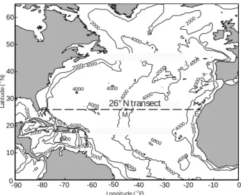
224 D. Cromwell et al.: Towards measuring the MOC from space M -90 -80 -70 -60 -50 -40 -30 -20 -10 0 0 10 20 30 40 50 60 2000 4000 4000 4000 2000 2000 2000 4000 2000 4000 4000 6000 2000 2000 2000 4000 4000 4000 6000 4000 2000 2000 4000 4000 4000 2000 6000 4000 26° N transect W E Longitude ( O E) L a ti tu d e ( ON )
Fig. 1. The region of study in which model output was extracted
from the Parallel Ocean Climate Model (POCM). Empirical orthog-onal functions of sea surface height anomaly and bottom pressure anomaly were calculated for the two subregions north and south of
the 26◦N transect. The corresponding terms in Eqs. (5) and (6) are
indicated by prefixes N and S. In addition, the location of the three
simulated in situ measurements on the 26◦N transect, also extracted
from POCM, are indicated by the prefixes W , M and E.
barotropic and baroclinic components) geostrophic flow, and thus allow an estimate of the full-depth mass transport of the MOC.
As there are currently insufficient satellite-derived bottom pressure data, we simulate satellite observations of bottom pressure using the Parallel Ocean Climate Model (POCM). We do the same for SSH. The initial task, which is the topic of this paper, is to test how well the MOC could be estimated using satellite observations alone. The basic method is to use a linear model to predict the MOC from the simulated satellite observations of bottom pressure and SSH.
We emphasise that this paper is a feasibility study show-ing that it is possible to estimate the strength of the MOC from space; but it does not demonstrate an actual working system. It will take considerable follow-up work, and an im-proved resolution gravity mission, before such a system can be produced.
2 Meridional overturning circulation
2.1 Introduction
The MOC is defined as the mass transport of water as a func-tion of latitude and depth. The MOC stream funcfunc-tion, 9, is: 9(y, z0, t ) = z0 Z −H L Z 0 v(x, y, z, t )dxdz (1)
where v=v(x, y, z, t ) is the meridional velocity; H =H (x, y) is the water depth; L=L(y, z) is the zonal width of the basin; and x, y, z and t are the longitude, latitude, depth and time coordinates.
2.2 Model description
Our proposed method of monitoring the MOC is tested here using output from POCM-4C, a global eddy-permitting model (Semtner and Chervin, 1992). This is an established and realistic ocean model covering a multidecadal time pe-riod. Its MOC has average values of around 20 Sv (1 Sver-drup or Sv = 106m3/s), consistent with in situ observations (Marsh et al., 2005).
POCM is on a Mercator geographical grid with a lon-gitudinal resolution of 0.4◦ and a latitudinal resolution of 0.4◦×cos(φ), where φ is latitude, yielding an average spa-tial resolution of 0.25◦. The bottom topography is derived from the 5-minute of arc resolution grid of the Earth To-pography dataset (ETOPO5). The model is forced with at-mospheric fluxes (wind stress, freshwater and heat) using the European Centre for Medium-Range Weather Forecasts (ECMWF) twenty-year reanalysis (i.e., ERA-15 reanalysis product + 5 years of consistent ECMWF operational fields processed with the same algorithms) data (Matano et al., 2002). The model run extends from Jan 1979 to Dec 1998, inclusive. The model was initialized from previous runs of the model (one 20-year simulation: see Stammer et al., 1996; and the initial 0.5◦simulation of Semtner and Chervin, 1992,
with a spin-up of 33 years).
POCM has twenty depth levels, and a free surface con-sistent with the formulation of Killworth et al. (1991). A description of the POCM equations and algorithms can be found in Stammer et al. (1996). The geographical region from which POCM output is extracted here is 0◦to 68◦N, 0◦to 90◦W (see Fig. 1). We use temperature, salinity, zonal (u) and meridional (v) velocities, as well as density.
To determine the realism of POCM, previous studies have compared the model with altimetry, hydrography and tide gauge observations (Stammer et al., 1996; Tokmakian, 1996; Tokmakian and Challenor, 1999). There was good agreement between POCM and hydrography at low latitudes of the At-lantic Ocean, where the rms difference was less than 7 cm (Stammer et al., 1996). The simulation of large-scale general circulation patterns was also realistic, although POCM gen-erally had weak circulation on all scales. For example, the eddy kinetic energy was four times lower in the model com-pared with altimetry data (Stammer et al., 1996). Tokmakian (1996) compared a nine-year time series of POCM sea sur-face heights with tide gauge records and found that the model gave realistic local sea level variability.
It must be stressed here that the present paper is a feasibil-ity study. Although, like all models, POCM is not a precise representation of the real ocean – notwithstanding that its MOC values in the North Atlantic are close to the observed
strength – it does provide a useful test bed for developing the statistical methodology, which we now describe in the fol-lowing section.
3 Methodology
3.1 Description of the statistical method
Our aim is to see if the MOC can be estimated from sim-ulated SSH and bottom pressure data from POCM output. Obtaining SSH is straightforward as it is output directly by the model. Bottom pressure, pH, is obtained from:
pH ∼= gρ0ζ + g 0
Z
−H
ρdz + pa (2)
where ζ is SSH and pa is the atmospheric pressure. We use
an average of four grid points for SSH and bottom pressure. Thus our bottom pressure data (∼100 km resolution) do not simulate the current GRACE satellite observations (∼400 km resolution), but a future higher resolution mission instead.
Rather than use complex non-linear fitting procedures, such as neural networks or support vector machines (Hastie et al., 2003), we use a linear model. Our statistical model is given by: MOCi = p X j =1 αjXij+εi (3)
where MOCi is the value of the MOC at the ith timestep,
αj are coefficients corresponding to the linear predictors
Xij(j =1, p), and εi is an error term such that:
εi ∼N (0, σ2) and E(εiεj) = 0, i 6= j (4)
In other words, the error terms belong to a Normal distribu-tion, N , with zero mean and standard deviadistribu-tion, σ ; and the error terms are assumed to be independent of each other; i.e. the expectation value, E, of cross-correlations of different error terms is 0.
The variables to be used as predictors in Eq. (3) need to be determined. Two sets of predictors are used: (1) a “geostrophic” set comprising SSH and bottom pressure val-ues at either end (79◦W and 15◦W) of the 26◦N basin tran-sect, and also at one point in the middle (45◦W; see Fig. 1); and (2) a “gyre” set comprising the first three empirical or-thogonal functions (EOFs) for both SSH anomaly and bot-tom pressure anomaly (BPA) over the whole region of Fig. 1, as well as the subregions north and south of 26◦N. The ratio-nale for the former set, i.e. (1), is clear. For the latter set, we exploit the suggestion by H¨akkinen and Rhines (2004) that EOFs provide a measure of the gyre strength. Using EOFs north and south of 26◦N, as well as for the whole basin, lows us to distinguish the subpolar and subtropical gyres, al-beit in a crude way. Equivalently, we may regard 26◦N as
the line of zero windstress curl, to a rough first approxima-tion. Note that, like most ocean general circulation models, POCM conserves volume rather than mass (McDougall et al., 2002). In order to reduce the effect of any change in mass that may influence our results, we detrended SSH and BP locally (i.e., gridpoint by gridpoint).
In the statistical model we allow interaction between the various SSH terms and between the various BPA terms. However, for simplicity, we do not allow interactions be-tween the SSH and BPA terms. Similarly, we do not allow in-teractions between the geostrophic terms and the gyre terms, or between the north, south or total gyre terms. H¨akkinen and Rhines (2004) investigated the possible role of the North At-lantic Oscillation (NAO) in the strength of the MOC. There-fore, we also include an NAO index in the model.
Our model notation in Eq. (5) follows that of Wilkin-son and Rogers (1973). Thus, “*” includes the interaction terms whilst “+” does not. Therefore, A*B+C, for exam-ple, means the terms A+B+A.B+C; and A*B*C indicates A+B+C+A.B+A.C+B.C+A.B.C. Our initial model is:
MOC = Constant + NAO
+Wssh ∗ Mssh ∗ Essh + Wbpa ∗ Mbpa ∗ Ebpa +Bssh 1 ∗ Bssh 2 ∗ Bssh 3 + Bbpa 1 ∗ Bbpa 2 ∗ Bbpa 3 +Nssh 1 ∗ Nssh 2 ∗ Nssh 3 + Nbpa 1 ∗ Nbpa 2 ∗ Nbpa 3
+Sssh 1 ∗ Sssh 2 ∗ Sssh 3 + Sbpa 1 ∗ Sbpa 2 ∗ Sbpa 3 (5)
where ssh is sea surface height anomaly, bpa is bottom pres-sure anomaly, the prefixes W , M, and E refer to the west, middle and east of the 26◦N transect, respectively. The
num-ber at the end of the term denotes the xth EOF. The prefix B means the EOF covers the whole basin, N is north of 26◦N
and S is south of 26◦N. A location map showing the region of interest is given in Fig. 1. The results are presented in Sect. 4.
3.2 EOF analysis
As explained above, to obtain the linear predictors needed for Eq. (3) we require an EOF analysis of the two POCM datasets. These are sea surface height anomaly and bottom pressure anomaly. In both cases, “anomaly” simply means calculated with respect to the respective time-mean of the model variable over the POCM run from January 1979 to December 1998, inclusive.
The EOF principal components (i.e. the time series asso-ciated with each EOF) are used as inputs for the linear re-gression model. We calculate EOFs of SSH anomaly for the complete North Atlantic basin using POCM output. We re-peat for the area north of 26◦N and also the area south of 26◦N. There is a secular trend in SSH anomaly principal component mode 1 (not shown), indicative of model drift. We address this below.
226 D. Cromwell et al.: Towards measuring the MOC from space
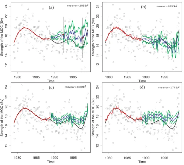
(a) rms error = 2.02 Sv2 (b) rms error = 0.63 Sv2
(c) rms error = 0.93 Sv2 (d) rms error = 1.74 Sv2
Fig. 2. The strength of the meridional overturning circulation in Sv at 26◦N in POCM (open black circles are monthly averages; black line is smoothed MOC: see text for details). Linear model fit (red line) for the training data, and predictions (blue line) with 95% standard errors of the prediction (green line) for (a) the simplest regression model; (b) using smoothed and partially detrended inputs for the model; (c) adding satellite-equivalent noise to the inputs; and (d) using smoothed and detrended SSHA only. The diamonds in (a) represent actual observations, with the vertical lines representing their respective error bars (Marsh et al., 2005).
4 Results
Figure 2a shows the monthly strength of the MOC in Sv over the years 1979–1998. There is strong month-to-month vari-ability. Our primary interest is in the long-term variation of the MOC, with most interest focusing on early warning of any imminent shutdown in the thermohaline circulation, rather than inter-month variation; therefore these MOC val-ues are smoothed appropriately. We apply a simple spline smoother (smooth.spline in the R language (R Development Core Team, 2004)). The smoothed MOC is shown as the solid black line in Fig. 2. The long-term behaviour of the MOC is apparent: after an initial rise, the MOC strength falls almost linearly until 1997 when it recovers close to its earlier maximum strength of 20 Sv. The reasons for this variability are as yet unknown.
We now fit the statistical model described in Sect. 3 to the
data shown in Fig. 2. We use a standard F-test for the linear model (Venables and Ripley, 2002) to see which terms are significant. Note that we do not fit the terms sequentially; we simply fit the most complex model described in Sect. 3. The input variables for the model are smoothed using the spline smoother. The statistical model explains 93.5% of the variability prior to smoothing the inputs, and 98% following smoothing. In none of our fits is the NAO significant. This is consistent with the finding of H¨akkinen and Rhines (2004) that the NAO is not a significant factor in the subpolar gyre weakening observed in the 1990s.
To test the strength of this model, we use the first half of the data as a training set to predict the MOC for the second half of the data. Using Eq. (5), the resulting fit explains 99% of the variability in the half of the data used for the fitting, but does not give a good prediction of the second half of the
data (Fig. 2a). The mean square error of this prediction is 2.02 Sv2. We believe this relatively poor prediction arises from drift in the model output, even though model output data had been previously detrended locally (i.e., gridpoint by gridpoint). Earlier, we mentioned that POCM conserves vol-ume rather than mass. It is possible for the model to gain or lose mass, which seems to have happened here. This likely affects the density structure of the ocean, influencing both the SSH and bottom pressure. In addition, this study only extracted a part of the Atlantic Ocean region from the global POCM dataset. Volume is not necessarily conserved in this subregion: thus, for example, a net loss of volume in the At-lantic Ocean will be compensated by a net gain somewhere else in the global ocean. Because volume is not conserved in the studied subregion there will be model drift, namely a trend in SSH. This is seen in the trend in the 1st EOF of SSH. Therefore, to correct for this model drift, in what follows we only use EOFs 2 to 4 for SSH: all terms involving the first EOF of SSH are removed. The mean square error of the pre-diction is now much improved to just 0.63 Sv2(Fig. 2b).
We also simulated the effect of random errors in the satel-lite data. It is well known that the typical rms precision and accuracy of TOPEX/POSEIDON altimetry is ∼2 cm. When we add 2 cm of noise to the detrended SSH model inputs, noise on the BPA data has very little effect on the error in the transport estimate. The results, using 0.02 mb of noise for bottom pressure (a realistic value for future space grav-ity missions) are shown in Fig. 2c. The mean square error for this prediction is 0.93 Sv2. Intriguingly, the noise on the BPA data makes little difference whereas the noise on SSH has a large effect. The reason for this can be seen from Eq. (6) where we have removed the non-significant terms.
MOC=Constant+Wsshs+Nssh 3s+Nssh 4s
+Bssh 2s.Bssh 4s+Nssh 2s.Nssh 3s+Sssh 2s.Sssh 3s
+Sssh 3s.Sssh 4s+Wsshs.Esshs+Wsshs.Msshs.Esshs
+Bbpa 2s+Bbpa 3s+Sbpa 1s+Bbpa 1s.Bbpa 2s +Bbpa 2s.Bbpa 3s+Nbpa 1s.Nbpa 2s+Sbpa 1s.Sbpa 3s
+Bbpa 1s.Bbpa 2s.Bbpa 3s+Wbpas.Ebpas
(6)
where the subscript “s” refers to a simple spline smoother applied to the parameters.
Equation 6 shows that the only significant BPA variables are the large scale EOFs. The noise on individual measure-ments do not affect these (white noise is taken up by the higher order EOFs). However, if we were to add geograph-ically correlated noise, as might be produced from a real satellite system, these would modify our results. The simu-lation of such errors is complex and is not considered in this paper.
Intriguingly, detrending the data before calculating the EOFs gives a worse prediction than detrending the EOFs themselves. In the former case we remove a separate trend for each grid point. This is probably removing relevant local information. On the other hand, working with the detrended EOFs tends to remove the large-scale trends that we expect to
be caused by non-conservation of mass. This model, which has the best predictive skill (as measured by the lowest mean square error of 0.63 Sv2), is that shown in Fig. 2b.
To test whether the model can produce the same result without bottom pressure, the model was run using only SSH terms and used to predict the MOC for the second half of the data. The results can be seen in Fig. 2d. The mean square error is 1.74 Sv2. Thus omitting the bottom pressure terms gives a significantly worse prediction (compare with Fig. 2b).
5 Discussion and future work
Our study suggests that it is possible to monitor the merid-ional overturning circulation (MOC) using a combination of sea surface height and bottom pressure measurements from space. The eventual aim of this work is an early warning system for possible collapse of the North Atlantic thermoha-line circulation. The considerable month-to-month variabil-ity means that we need to extract carefully the trend from the signal; otherwise many false alarms would be triggered.
The linear regression method explains 98% of the vari-ability in the smoothed MOC when the inputs are smoothed. In fitting the regression we assumed that the residuals were uncorrelated. This is true for the unsmoothed data but the smoothing adds correlation and non-white residual noise. This noise has a rather complex structure and our attempts to model it using ARMA noise models have so far been un-successful. However, the successful prediction of the second, unfitted, half of the data shows that our model is robust, al-though the estimated errors are likely too low.
We have used the Parallel Ocean Climate Model (POCM) in this paper. It would clearly be useful to test the pro-posed method on other models also, such as OCCAM (Webb, 1996), HYCOM (Chassignet et al., 2003) or HadCM3 (Gor-don et al., 2000), and also by exploiting high-resolution grav-ity data from space, probably from a follow-up GRACE mis-sion. Once the MOC monitoring array near 26◦N has been fully operational for some time we hope to compare it with our satellite-based method. Such a test will only be use-ful once a sufficiently long time series becomes available: perhaps ∼10 years, as suggested by our prediction testing. We intend to repeat our studies at additional latitudes to test whether our methodology can be applied to monitor the MOC at locations other than that of the RAPID array, thus complementing and extending the array’s capability.
Acknowledgements. We gratefully acknowledge useful suggestions
and feedback from colleagues at NOCS, especially J. Hirschi and B. Sinha, and from the reviewers. This work was initially funded under the Rapid Climate Change thematic programme of the UK’s Natural Environment Research Council.
228 D. Cromwell et al.: Towards measuring the MOC from space
References
Bryden, H. L., Longworth, H. R., and Cunningham, S. A.:
Slow-ing of the Atlantic meridional overturnSlow-ing circulation at 25◦N,
Nature, 438, 655–657, 2005.
Chassignet, E. P., Smith, L. T., Halliwell, G. R., and Bleck, R.: North Atlantic simulation with the HYbrid Coordinate Ocean Model (HYCOM): Impact of the vertical coordinate choice, ref-erence density, and thermobaricity, J. Phys. Oceanogr., 33, 2504– 2526, 2003.
Gordon, C., Cooper, C., Senior, C. A. , Banks, H.T., Gregory, J. M., Johns, T. C., Mitchell, J. F. B., and Wood, R. A.: The simulation of SST, sea ice extents and ocean heat transports in a version of the Hadley Centre coupled model without flux adjustments, Clim. Dyn., 16, 147–168, 2000.
Gregory, J. M., K. W. Dixon, R. J. Stouffer, A. J. Weaver, E. Driess-chaert, M. Eby, T. Fichefet, H. Hasumi, A. Hu, J. H. Jungclaus, I. V. Kamenkovich, A. Levermann, M. Montoya, S. Murakami, S. Nawrath, A. Oka, A. P. Sokolov, and R. B. Thorpe: A model intercomparison of changes in the Atlantic thermohaline
circu-lation in response to increasing atmospheric CO2concentration,
Geophys. Res. Lett., 32, L12703, doi:10.1029/2005GL023209, 2005.
H¨akkinen, S.: Variability in sea surface height: A qualitative mea-sure for the meridional overturning in the North Atlantic, J. Geo-phys. Res., 106, 13 837–13 848, 2001.
H¨akkinen, S. and Rhines, P. B.: Decline of Subpolar North Atlantic Circulation During the 1990s, Science, 304, 555–559, 2004. Hastie, T., Tibshirani, R., and Friedman, J.: The Elements of
Statis-tical Learning: Data Mining, Inference and Prediction. Springer, 2003.
Hirschi, J, Baehr, J., Marotzke, J., Stark, J., Cunningham, S., and Beismann, J.-O.: A monitoring design for the Atlantic Merid-ional Overturning Circulation, Geophys. Res. Lett., 30(7), 1413, doi:10.1029/2002GL016776, 2003.
Killworth, P. D., Stainforth, D., Webb, D. J., and Patterson, S. M.: The development of a free-surface Bryan-Cox-Semtner ocean model, J. Phys. Oceangr., 21, 1333–1348, 1991.
Levermann, A., Griesel, A., Hofmann, M., Montoya, M., and Rahmstorf, S.: Dynamic sea level changes following changes in the thermohaline circulation, Clim. Dyn., 24, 347–354, 2005. McDougall, T. J., Greatbatch, R. J., and Lu, Y.: On
conserva-tion Equaconserva-tions in Oceanography: How Accurate are Boussinesq Ocean Models?, J. Phys. Oceangr., 32, 1574–1584, 2002. Marsh, R., de Cuevas, B. A., Coward, A. C., Bryden, H. L., and
Al-varez, M.: Thermohaline circulation at three key sections in the North Atlantic over 1985-2002, Geophys. Res. Lett., 32, L10604, doi:10.1029/2004GL022281, 2005.
Matano, R. P., Beier, E. J., Strub, P. T., and Tokmakian, R.: Large-scale forcing of the Agulhas variability: The seasonal cycle, J. Phys. Oceangr., 32, 1228–1241, 2002.
R Development Core Team: R: A language and environment for statistical computing, R Foundation for Statistical Computing, Vienna, Austria, http://www.R-project.org, 2004.
Rahmstorf, S.: Thermohaline Ocean Circulation, in Encyclopedia of Quaternary Sciences, edited by: Elias, S. A., Amsterdam, El-sevier, 2006.
Rahmstorf, S. and Ganopolski, A.: Long-term global warming sce-narios computed with an efficient coupled climate model, Clim. Change, 43, 353–367, 1999.
Semtner, A. J. and Chervin, R. M.: Ocean general circulation from a global eddy-resolving model, J. Geophys. Res., 97, 5493–5550, 1992.
Stammer D., Tokmakian, R., Semtner, A., and Wunsch, C.: How
well does a 1/4◦ global circulation model simulate large-scale
oceanic observations? J. Geophys. Res., 101(C10), 25 779–
25 811, 1996.
Stocker, T. F., Knutti, R., and Plattner, G.-K.: The Future of the Thermohaline Circulation – A Perspective in The Oceans and Rapid Climate Change: Past, Present and Future, edited by: Bar-ron, E. J. and Seidov, D., American Geophysical Union. Geo-physical Monograph., 126, 277–293, 2001.
Tapley, B. D., Chambers, D. P., Bettadpur, S., and Ries, J. C.: Large scale ocean circulation from the GRACE GGM01 Geoid, Geophys. Res. Lett., 30(22), 2163, doi:10.1029/2003GL018622, 2003.
Tapley B. D., Bettadpur, S., Watkins, M., and Reigber,
C.: The gravity recovery and climate experiment: Mission overview and early results, Geophys. Res. Lett. 31, L09607, doi:10.1029/2004GL019920, 2004a.
Tapley, B. D., Bettadpur, S., Ries, J. C., Thompson, P. F., and Watkins, M. M.: GRACE Measurements of Mass Variability in the Earth System, Science, 305, 503–505, 2004b.
Tokmakian, R.: Comparisons of time series from two global models with tide-gauge data, Geophys. Res. Lett., 23(25), 3759–3762, 1996.
Tokmakian, R. and Challenor, P. G.: On the joint estimation of model and satellite sea surface height anomaly errors, Ocean Modell., 1, 39–52, 1999.
Venables, W. N. and Ripley, B. D.: Modern Applied Statistics with S, Springer, New York, 2002.
Wahr, J. and Molenaar, M.: Time variability of the Earth’s gravity field: Hydrological and oceanic effects and their possible detec-tion using GRACE, J. Geophys. Res., 103(B12), 30 205–30 229, 1998.
Webb, D. J.: An ocean model code for array processor computers, Comput. Geosci., 22, 569–578, 1996.
Wilkinson, G. N. and Rogers, C. E.: Symbolic description of facto-rial models for analysis of variance, Appl. Statist., 22, 392–399, 1973.
Wood, R. A., Keen, A. B., Mitchell, J. F. B., and Gregory, J. M.: Changing spatial structure of the thermohaline circulation in
re-sponse to atmospheric CO2forcing in a climate model, Nature,
399, 572–575, 1999.