The Heidelberg iterative cloud retrieval utilities (HICRU) and its application to GOME data

(1)

HAL Id: hal-00301053

https://hal.archives-ouvertes.fr/hal-00301053

Submitted on 7 Mar 2006

HAL is a multi-disciplinary open access

archive for the deposit and dissemination of sci-entific research documents, whether they are pub-lished or not. The documents may come from teaching and research institutions in France or abroad, or from public or private research centers.

L’archive ouverte pluridisciplinaire HAL, est destinée au dépôt et à la diffusion de documents scientifiques de niveau recherche, publiés ou non, émanant des établissements d’enseignement et de recherche français ou étrangers, des laboratoires publics ou privés.

The Heidelberg iterative cloud retrieval utilities

(HICRU) and its application to GOME data

M. Grzegorski, M. Wenig, U. Platt, P. Stammes, N. Fournier, T. Wagner

To cite this version:

M. Grzegorski, M. Wenig, U. Platt, P. Stammes, N. Fournier, et al.. The Heidelberg iterative cloud retrieval utilities (HICRU) and its application to GOME data. Atmospheric Chemistry and Physics Discussions, European Geosciences Union, 2006, 6 (2), pp.1637-1678. �hal-00301053�

(2)

ACPD

6, 1637–1678, 2006 Application of HICRU to GOME data M. Grzegorski et al. Title Page Abstract Introduction Conclusions References Tables Figures J I J I Back Close

Full Screen / Esc

Printer-friendly Version Interactive Discussion

EGU

Atmos. Chem. Phys. Discuss., 6, 1637–1678, 2006 www.atmos-chem-phys-discuss.net/6/1637/2006/ © Author(s) 2006. This work is licensed

under a Creative Commons License.

Atmospheric Chemistry and Physics Discussions

The Heidelberg iterative cloud retrieval

utilities (HICRU) and its application to

GOME data

M. Grzegorski1, M. Wenig2, U. Platt1, P. Stammes3, N. Fournier3, and T. Wagner1

1

Institute of Environmental Physics, University of Heidelberg, Germany 2

NASA Goddard Space Flight Center, Greenbelt, Maryland, USA 3

KNMI, Climate Research and Seismology Department, de Bilt, The Netherlands Received: 23 December 2005 – Accepted: 9 February 2006 – Published: 7 March 2006 Correspondence to: M. Grzegorski (mgrzegor@iup.uni-heidelberg.de)

(3)

ACPD

Full Screen / Esc

EGU

Abstract

Information about clouds, in particular the accurate identification of cloud free pixels, is crucial for the retrieval of tropospheric vertical column densities from space. The Hei-delberg Iterative Cloud Retrieval Utilities (HICRU) retrieve effective cloud fraction using spectra of two instruments designed for trace gas retrievals from space: The Global

5

Ozone Monitoring Experiment (GOME) on the European Remote Sensing Satellite (ERS-2) and the SCanning Imaging Absorption SpectroMeter for Atmospheric CHar-tographY (SCIAMACHY) on ENVISAT.

HICRU applies the widely used threshold method to the so-called Polarization Moni-toring Devices (PMDs) with higher spatial resolution compared to the channels used for

10

trace gas retrievals. Cloud retrieval and in particular the identification of cloud free pix-els is improved by HICRU through a sophisticated, iterative retrieval of the thresholds which takes their dependency on different instrumental and geometrical parameters into account. The lower thresholds, which represent the surface albedo and strongly affect the results of the algorithm, are retrieved accurately through a four stage

classi-15

fication scheme using image sequence analysis.

The design and the results of the algorithm applied to GOME data are described and compared to several other cloud algorithms for GOME. The differences to other cloud algorithms are discussed with respect to the particular characteristics of the al-gorithms.

20

1 Introduction

The detection of cloud parameters like cloud coverage, cloud top pressure or cloud optical thickness from satellite is an important issue: 1.) for meteorology and the in-vestigation of climate change and 2.) for the analysis of tropospheric trace gases from space relevant to environmental and climatological issues. Although the retrieval of

dif-25

(4)

iden-ACPD

Full Screen / Esc

EGU

tification of completely cloud free regions is crucial due to the shielding effect, which causes an underestimation of the vertical column density of tropospheric trace gases measured by satellite.

1.1 The Global Ozone Monitoring Experiment

The Global Ozone Monitoring Experiment (GOME) (Burrows et al., 1999) on board

5

the ESA satellite ERS-2 provides data for the retrieval of vertical column densities of tropospheric trace gases (e.g. NO₂, SO₂, HCHO, H₂O) using the DOAS technique

(Platt, 1994; Burrows et al., 1999; Wagner et al., 2002). The satellite flies along a

sun-synchronous polar orbit at an altitude of about 780 km and crosses the equator at 10:30 a.m. (local time). Global coverage is achieved every three days. The orbit

10

of the satellite leads to an essentially constant relationship between the solar zenith angle and the latitude depending only on the seasonal shift in the position of the sun. GOME measures earthshine spectra in a nadir viewing geometry, i.e. it looks radi-ally towards the earth. The earth’s surface is scanned with an angular range of 31◦ both in western and eastern direction corresponding to a cross track swath width of

15

960 km. During each scan three subpixels are mapped extending 320 km east-west and 40 km north-south: subpixel 0 (east), subpixel 1 (center) and subpixel 2 (west). These three forescan pixels are followed by a backscan pixel (subpixel 3) with an ex-tent of 960*40 km2. GOME consists of four spectrometers in UV/vis wavelength region with moderate spectral resolution (0.2–0.4 nm) used for the DOAS retrieval of trace

20

gases. Furthermore, the GOME instrument bears three broad band detectors covering the UV (PMD1, 295–397 nm) and the visible wavelength region (PMD2, 397–580 nm and PMD3, 580–745 nm). These Polarization Monitoring Devices (PMDs) are mainly intended for measuring the polarization of the observed light. However, the PMDs can be read out more frequently than the channels with moderate spectral resolution.

25

Thus, we receive 16 PMD measurements across each subpixel. This results in a higher spatial resolution of 20×40 km2(instead of 320×40 km2), which makes the PMDs

(5)

es-ACPD

Full Screen / Esc

EGU

pecially suitable for an intensity-based cloud retrieval from GOME data (see Sect.2). 1.2 Cloud retrieval from GOME data

There are already several algorithms retrieving cloud parameters from GOME data: The official GOME cloud product ICFA (Initial Cloud Fitting Algorithm, Kuze and

Chance, 1994) and the FRESCO algorithm (Fast REtrieval Scheme for Clouds from

5

the Oxygen-A-Band,Koelemeijer et al.,2001) use the GOME channels with moderate spectral resolution. There are also several algorithms using the PMD instruments (see Table2, Sect. 4).

Two different quantities are typically applied for cloud retrieval from GOME data: The first class of algorithms use the absorption of the O₂-A-Band: Since clouds reduce the

10

penetration of light down to low layers of the atmosphere, the absorption of oxygen is reduced for a cloudy pixel compared to a cloud free measurement, where the ab-sorption mainly depends on cloud coverage, cloud albedo and cloud top height. This approach is used by ICFA and FRESCO, but cannot be applied to the PMD instruments because of their insufficient spectral resolution. The major idea of the second class of

15

algorithms is, that clouds can also be identified through the intensity of reflected light hardly effected by trace gas absorptions, because clouds are usually brighter than the surface. These intensities are mainly independent of cloud top height, but they also depend on cloud coverage and cloud albedo. This approach is applied using small spectral windows of the detectors with moderate spectral resolution (FRESCO) and

20

by the algorithms using the PMD instruments (Table2, Sect. 4). All these algorithms retrieve an effective cloud fraction, a parameter that combines cloud coverage (cloud abundance) of the pixel and cloud albedo.

The first class of algorithms is used in two different ways: ICFA retrieves effective cloud fraction using the absorption of the O₂-A-band directly, where the cloud top

25

height is defined a priori using the ISCCP climatology (Schiffer and Rossow, 1983). This can create large errors in cloud fraction if the cloud top height deviates from the climatological average (Koelemeijer and Stammes,1999). On the other hand, the O₂

(6)

-ACPD

Full Screen / Esc

EGU

A-band approach is also used to retrieve cloud top height, where a combination of both approaches is used: an intensity-based effective cloud fraction is retrieved simul-taneously (FRESCO) or beforehand (GOME Cloud retrieval AlgoriThm ; GOMECAT,

v. Bargen et al.,2000, Retrieval Of Cloud Information by a Neural Network; ROCINN,

Loyola,2004).

5

There are further cloud algorithms designed for other satellite platforms, which can also be applied to GOME data. The Semi-Analytical CloUd Retrieval Algo-rithm (SACURA) retrieves cloud top height and further cloud parameters using the O₂-A-Band approach (Kokhanovsky et al.,2003; Rozanov and Kokhanovsky, 2004). SACURA is mainly developed for SCIAMACHY, but can also be applied to GOME data.

10

The method is limited to totally cloudy pixels and the algorithm has to be combined with other data products providing cloud coverage for application to partly cloudy pixels.

Besides the methods described above, further quantities, e.g. the absorption bands of O₄and the Ring effect can be used for the retrieval of cloud parameters from GOME data (Wagner et al., 2003; Beek et al., 2001) . These methods are used by two

al-15

gorithms developed for the Ozone Monitoring Instrument (OMI) on the AURA platform

(Acarreta et al.,2004;Joiner et al.,2004). Both algorithms are also applied to selected

GOME data for validation purposes.

2 The Heidelberg Iterative Cloud Retrieval Utilities (HICRU)

The HICRU algorithm uses the PMDs of GOME to retrieve the effective cloud

frac-20

tion, because of their higher spatial resolution compared to the channels with mod-erate spectral resolution. An important advantage of the higher spatial resolution is founded in the strong influence of the surface albedo on the retrieved cloud fraction

(Wenig,2001). The determination of surface albedo requires an adequately large set

of measurements referring to cloud free scenarios, but the probability of a cloud free

25

measurement strongly depends on spatial resolution.

(7)

ACPD

Full Screen / Esc

EGU

trace gases (e.g.Beirle et al.,2004a,b,c). This requires a decrease of the spatial res-olution to the pixel size of the channels with moderate spectral resres-olution, but we can retrieve at least an additional parameter describing cloud heterogeneity and obtain ad-ditional information about the spatial structure of cloud clusters. This is demonstrated by Fig.1. Nevertheless, HICRU is also applied to studies directly focussed on cloud

5

properties. An example is the analysis of the El-Ni ˜no phenomenon (Wagner et al.,

2005). In this case we directly benefit from the higher spatial resolution of the PMD instruments.

2.1 Application of the threshold method

The HICRU algorithm is based on the widely used threshold method. First, lower

10

thresholds I_cloudfree, representing the intensity of cloud free pixels, and upper thresholds

I_cloudy, representing the intensity of completely cloudy pixels, are calculated. The cloud

fraction CF is retrieved from the measured intensity I_meas through linear interpolation between the thresholds:

CF = Imeas− Icloudfree

I_cloudy− I_cloudfree (1)

15

This interpolation assumes a cloud to be lambertian reflector and a GOME pixel that can be divided into a cloud free part and a cloudy part, where the albedo of the cloudy part is implicitly determined by the upper thresholds. HICRU uses earthshine radiances divided by the cosine of the solar zenith angle and the daily solar spectrum. The accuracy of PMD cloud algorithms critically depend on the quality of the

calcu-20

lated lower and upper thresholds. The accurate retrieval of the the lower thresholds are especially important for the detection of cloud free pixels, because the measured intensity is not only sensitive to the cloud coverage and the cloud albedo, but also to the surface albedo, which depends on surface type and the season of the measure-ment. The lower thresholds are mainly determined by the surface albedo, but also

in-25

(8)

ACPD

Full Screen / Esc

EGU

pixels through intercomparison between cloudy and clear-sky top-of-atmosphere ra-diances. The major advantage of the HICRU algorithm is the improvement of cloud retrieval through an iterative retrieval of thresholds, including image sequence analysis for the retrieval of the lower threshold. The algorithms for the retrieval of thresholds are described in Sect.3in detail and make an accurate cloud retrieval also possible for

5

regions like deserts, which often cause to problems for other GOME cloud algorithms (Sect.4).

2.2 PMD detectors used for cloud retrieval

HICRU can be applied to all PMD channels, but we chose to use the sum of the inten-sities of PMD 2 (397–580 nm) and PMD 3 (580–745 nm) for cloud retrieval because of

10

the following considerations: The propagation of errors in the lower thresholds to cloud fraction depends strongly on the intensity difference between the upper and the lower threshold. In desert regions, cloud fraction calculated from PMD 3 is more sensitive to errors in the lower threshold than cloud fraction retrieved from PMD 2, because the albedo of the desert is higher in the wavelength region covered by PMD 3. Obviously it

15

is the other way around for ocean. Hence the combined use of PMD 2 and PMD 3 was found to be a good compromise for different regions on earth. We should not switch between the used channels depending on surface albedo, because the obtained upper threshold and the instrument degradation also differ between the channels. Because of the strong degradation effects, in particular, for PMD 1 (Aben et al.,2000; Krijger 20

et al., 2005) this channel is omitted in HICRU. Further reasons for the exclusion of PMD1 are the strong sensitivity to the polarization of the earth radiance (Schutgens

and Stammes, 2003) and the strong impact of Rayleigh-scattering in the UV-region covered by this detector.

(9)

ACPD

Full Screen / Esc

EGU

2.3 Color space analysis is not used by HICRU

Some PMD algorithms make use of color space analysis additionally to the intensity-based approach (e.g. the Optical Cloud Recognition Algorithm – OCRA, v. Bargen

et al., 2000 – and the Cloud Retrieval algorithm Using image Sequence Analysis – CRUSA,Wenig,2001). The intensities of the three PMDs are interpreted as three

dif-5

ferent colors (red, green and blue) in the RGB colorspace. The main idea is to use the different color characteristics of clouds and the surface. This can be done by an-alyzing different parameters like the saturation in the HSV color space (Wenig,2001), which is determined on the basis of the ratio of the PMDs with the lowest and the highest intensities. We do not include this approach in our retrieval for different

pur-10

poses: as discussed above, the UV channel should be omitted and a switch between the PMD channels should be avoided. Furthermore, if the cloud fraction is retrieved through interpolation between the thresholds a cloud model is implicitly assumed: An intensity-based cloud fraction refers to a lambertian cloud and the cloud fraction can be interpreted as a physical quantity of measurement linearly proportional to cloud albedo

15

and cloud coverage. It is particularly important to know the relation of the retrieved cloud fraction to these parameters for combining the HICRU cloud fractions with other data like the absorption by O₂and O₄for the retrieval of further cloud parameters like cloud top height. This will we be realized by algorithms currently in development. For color characteristics the quantitative relation to physical quantities like cloud albedo

20

is unknown. If we retrieve an intensity-based cloud fraction, the lower threshold rep-resents the intensity of a cloud free measurement, which is lower than in the cloudy case. We found that the retrieval is not predominantly limited by identification of cloud free pixels, but by the lack of measurements of cloud free scenarios.

(10)

ACPD

Full Screen / Esc

EGU

3 Retrieval of HICRU thresholds

3.1 Thresholds for cloud free pixels

The lower threshold strongly depends on surface albedo and has to be calculated with respect to the latitude and longitude of measurement. We have to retrieve a map of the earth containing minimum reflectances of the sum of PMD2 and PMD3 as lower

5

thresholds. Two different strategies could be applied: on the one hand, we should use short periods of time for the retrieval, because of seasonal variations of the surface albedo and the effects of irregular instrument degradation dependent on the time of measurement. Hence we should aim to retrieve maps representing the lower thresh-old separately for each day using periods as short as possible (HICRU uses 25 days).

10

On the other hand, this method only would work appropriately if cloud free pixels ex-ist during the considered period of time. This assumption holds well for regions like the Sahara, but is hardly acceptable for regions with persistent or seasonal cloud cov-erage. Note, that GOME needs three days to cover the earth completely, thus there are not more than 9 measurements during 25 days for some regions on earth and the

15

possibility that all of them are cloudy is not negligible. To take both strategies into ac-count, HICRU uses a four stage classification scheme analyzing both long and short periods of time (see Table1). It is particularly interesting to note that the reflectance of the PMDs depends systematically on the GOME subpixel. Hence we retrieve the thresholds separately for the four subpixels of GOME.

20

HICRU uses an iterative algorithm similar to CRUSA (Wenig,2001) based on image sequence analysis for all four stages of threshold retrieval. The main idea is to retrieve accumulation points of low intensities instead of the absolute minimum during the con-sidered period of time. This approach has at least three advantages: First the algorithm is more robust against errors in level-1 data, especially if long periods of time are

con-25

sidered, because the result is not determined by one measurement alone. Moreover, the accumulation point method can take the seasonal variation of the albedo during the considered period of time into account, if there exist more than one measurement

(11)

ACPD

Full Screen / Esc

EGU

corresponding to cloud free pixels: the average of the intensities for cloud free scenar-ios is a better choice than the absolute minimum in this case. The third advantage is, that the minimum reflectance retrieved by an accumulation point method during long periods can be used as a pre-classification criterion for the analysis of short periods of time: Using long periods, we can identify all clouds which raise the intensity steeply to

5

distinguish them from a variation of the surface albedo during the considered period of time. The assumed maximum variation of the surface albedo is pre-defined.

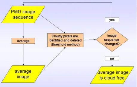
The principle of the iterative fixpoint algorithm is shown in Fig. 2. The algorithm is initialized by building up a set of daily global images containing the sum of the re-flectances from PMD2 and PMD3, whereas all pixels with intensities clearly brighter

10

than the Sahara are skipped. Each point of the image is now compared to the average image retrieved from the whole sequence. If the intensity of a measurement exceeds the sum of the average value and a pre-defined threshold, the measurement is inter-preted as cloudy and skipped from the sequence. The result is an image sequence containing less clouds. This sequence is used as input to run the algorithm again.

15

This is repeated until the image sequence does not change anymore. During stage 1, this algorithm is applied to the whole data set of GOME measurements from 1996 to 2003. The result is used as input for the second stage and the average of this im-age sequence (Fig.3) can be interpreted as first approximation of the lower threshold. During stage 2, 3 and 4 the algorithm is applied to gradually smaller sets of GOME

20

data (see Table1). After the fourth stage we obtain individual thresholds for each day, given by the average of the 25 days considered. An example for subpixel 2 is shown in Fig.4. This image contains several gaps corresponding to points, where no cloud free pixel is found during the 25 days1 (i.e., no value is left in the final image sequence). In this case, the algorithm has to use the average of the image sequences obtained

25

1

In practice, only 9 days of data are considered, because the earth is covered completely by GOME every three days only. Note, that an orbit only approximately covers the same regions of the earth as the corresponding orbits three days earlier or later. Because of this, it is not appropriate to consider periods longer than 25 days during stage 4

(12)

ACPD

Full Screen / Esc

EGU

from the earlier stages. Figure 4 shows, that stage 4 can be used over deserts, but not for most other regions on earth. On the other hand, errors in the retrieved albedo lead to errors in cloud fraction, especially for deserts, because of the high albedo in the wavelength region used by HICRU. This makes higher precision over deserts useful. Nevertheless, HICRU uses the stage covering the shortest period of time that includes

5

cloud free pixels (spatial resolution of the threshold images: 0.5·0.5◦) 3.2 Thresholds for cloudy pixels

The upper threshold represents a completely cloudy pixel for a cloud with high albedo. Image sequence analysis is not necessary for the retrieval, because the thresholds do not depend on surface albedo. Therefore we retrieve the upper threshold

depen-10

dent on solar zenith angle and GOME subpixel only. The algorithm works similar to the retrieval of the lower threshold (Fig. 2), but is applied separately to 1024 di ffer-ent data sets of PMD-measuremffer-ents: Each data set covers PMD-measuremffer-ents for a solar zenith angle bin of 2◦ (overall 32 bins). Separate data sets are used for each year of GOME data and the four subpixels of GOME. The algorithm starts with all

15

PMD-measurements from one of these data sets, whereas pixels definitely not rep-resenting completely cloudy pixels are skipped through a threshold method used for pre-classification. Afterwards, each measurement of the data set is compared with the average of all measurements. If a measurement underestimates the average of all measurements by more than predefined absolute and relative thresholds, it is removed

20

from the data set. The result is a reduced list of PMD measurements, which are used to run the algorithm again. This is repeated until the list does not change anymore. The results show a significant dependency of the retrieved thresholds on both solar zenith angle and subpixel (Fig.5).

The choice of the algorithm’s tuning parameters have to be selected carefully to

ob-25

tain a smooth correlation between the upper threshold and the solar zenith angle with-out with-outliers due to events of single, bright measurements from clouds or ice surfaces. We use huge data sets (a whole year) in order to be mostly independent of

(13)

climato-ACPD

Full Screen / Esc

EGU

logical dependencies and robust to errors in the PMD data. A single measurement with very high intensity should hardly affect the result. The upper threshold represents completely cloudy pixels with a high, but not maximum or explicitly defined or retrieved albedo. Clouds with higher albedo than the “model cloud” represented by the upper threshold are interpreted as cloud fractions higher than 1 by HICRU.

5

Ice and snow covered surfaces can be brighter than clouds with high albedo. For the retrieval of the upper thresholds different, pre-defined regions usually covered by snow or ice are skipped.

4 Intercomparison of HICRU to other cloud algorithms

New cloud algorithms have to be validated through intercomparison with existing cloud

10

datasets. These intercomparisons have to be done carefully especially for effective cloud fractions, because most data sets retrieved from other satellite platforms or sur-face observations do not provide an effective cloud fraction as defined for GOME cloud algorithms, but a cloud coverage retrieved for other assumptions on different cloud properties. Hence the GOME cloud fractions retrieved from HICRU and other cloud

al-15

gorithms cannot be compared directly to, e.g., ISCCP (Schiffer and Rossow,1983) or to meteorological cloud coverage from surface observation. HICRU can be compared to other GOME cloud algorithms or one of the few other cloud products from other satellites retrieving effective cloud fractions. Nevertheless, this paper concentrates on the intercomparison between different cloud algorithms for GOME and the different

20

approaches of the algorithms are discussed with respect to the results. For some of the cloud algorithms analyzed in this paper, intercomparisons are also discussed in

(14)

ACPD

Full Screen / Esc

EGU

4.1 Description of other cloud algorithms

All GOME cloud algorithms retrieve effective cloud fraction and in some cases addi-tional cloud parameters like cloud top height (see Sect.1.2). From a technical point of view, two different methods are used for the retrieval of cloud fraction. The first method is the threshold method (see Sect.2.1), which is used by the PMD algorithms. For the

5

intercomparison with HICRU, we included several PMD algorithms with different im-plementations of the threshold method, which lead to significant differences between the algorithms (Table 2). The second method is applied to the channels with mod-erate spectral and lower spatial resolution and is used to retrieve cloud fractions by ICFA and FRESCO. While the threshold method is founded completely on an empirical

10

base, the latter approach makes use of a radiative transfer model. Cloud fraction and, in the case of FRESCO, also cloud top height are retrieved using a χ2-minimization between the measured and the modelled spectra in and around the O₂-A-Band. The GOME pixel of 320×40 km is artificially divided into a cloud free and a cloudy part, where for the cloudy part a constant albedo is assumed a priori (FRESCO: 80%). For

15

radiative transfer modelling, a lambertian cloud is assumed and Rayleigh scattering is neglected.

The definition of cloud fraction in FRESCO is quite similar to the concept used by HICRU and the other PMD algorithms: both algorithms retrieve an effective, intensity-based cloud fraction with respect to a cloud with high albedo. But while this cloud

20

albedo is arbitrarily set to 80% by FRESCO, it is assumed indirectly for HICRU by re-trieving the upper threshold. For this reason, it is especially interesting to compare the results from HICRU with FRESCO, because on the one hand, both types of al-gorithms use a similar concept of effective cloud fraction, but on the other hand, dif-ferent detectors on the same satellite instruments and completely different retrieval

25

algorithms are used. Furthermore, FRESCO is an established and well validated al-gorithm (e.g. Koelemeijer and Stammes, 2000; Koelemeijer et al., 2002). Besides the intercomparison for one orbit including all described cloud algorithms (Sect. 4.2),

(15)

ACPD

Full Screen / Esc

EGU

we also include a detailed intercomparison between HICRU and FRESCO using one month of GOME data (Sect.4.3). During the development of this paper a new version of the FRESCO algorithm (see alsoFournier et al.,2006) has become available, which makes use of a better surface albedo database (Koelemeijer et al.,2003) and uses an improved calibration of the spectral data. We use the new database, but include both

5

FRESCO versions for some of the studies.

4.2 Correlation of HICRU with other cloud algorithms for GOME orbit 70716086 We analyzed the representative orbit 70716086 (16 July 1997) with respect to the results from HICRU and all the other algorithms described above. The orbit covers different kinds of surfaces: ocean, rain forest in central Africa, the Sahara and East

10

Europe. We found, that overall the cloud fraction is described in a similar way by all cloud algorithms (Fig. 6). But also substantial differences are found. These are analyzed in detail in the following subsections.

4.2.1 General differences between the algorithms

We correlated the results of all algorithms to those of HICRU. The highest correlation

15

coefficient (0.987) and the smallest standard deviation (0.033) is found for the PMD test algorithm, which was implemented by the HICRU developers to constitute the de-sign of HICRU (see Table2) and it is included in the intercomparison to support the interpretation of the data. Although there is strong correlation between HICRU and the more simple test algorithm, the improvement of HICRU for the retrieval of cloud free

20

pixels can be seen directly from the correlation: The significant reduction of negative cloud fractions is an improvement in the cloud retrieval, because both algorithms use an accumulation point method for the retrieval of the thresholds. The cloud fraction becomes negative, if the measured intensity is smaller than the lower threshold. Note, that only the CRUSA algorithm plots negative cloud fractions beside HICRU and the

25

(16)

ACPD

Full Screen / Esc

EGU

to 0, if the measured intensity is less than the lower threshold.

A similar high correlation as for the PMD test algorithm is also found for GOMECAT (0.976, see Table3). For both algorithms the correlation to HICRU is significantly higher than for the others (<0.94).

We found a correlation coefficient lower than 0.9 for only two of the analyzed

algo-5

rithms: ICFA (0.867) and the old FRESCO version (0.828). The old FRESCO version retrieves albedo information using two months of GOME data only, which is smaller than the data sets used for the retrieval of the lower threshold by all PMD algorithms. The seasonal variation of surface albedo is not taken into account. The new FRESCO version uses the database (Koelemeijer et al.,2003), which retrieves monthly albedo

10

maps based on 5 months of GOME data each. Because of the higher correlation co-efficient for the new FRESCO version (0.916), we ascribe the relatively low correlation coefficient of the old version to the shortcomings of the old FRESCO version compared to the new one. The correlations of both FRESCO versions to HICRU are significantly higher (0.921/0.964) if desert regions are neglected. This is explained in Sect.4.2.3.

15

The relatively low correlation of ICFA with HICRU is ascribed to the well-known short-comings of the ICFA algorithm (Sect.1.2).

For OCRA, GOMECAT(ISCCP), CRUSA and FRESCO we found a correlation co-efficient between 0.91 and 0.94. Note, that the standard deviation of the linear fit is significantly lower (0.089) for FRESCO than for the correlation of the three other

al-20

gorithms with HICRU. Nevertheless, these four algorithms mainly differ qualitatively from HICRU for very high or very low cloud fractions. CRUSA sometimes retrieves negative cloud fractions (typically between 0.0 and −0.2, sometimes up to −0.4) for HICRU cloud fractions lower than 0.15. This problem is due to inappropriate assump-tions for the interpolation between the lower and the upper threshold in HSV-color

25

space, which results in difficulties for regions with high saturation values of the lower threshold (especially over ocean). This problem of CRUSA is significantly improved, if regions completely or partly covered by ocean are neglected (Fig. 7). OCRA and GOMECAT(ISCCP) retrieve significant higher cloud fractions than HICRU, but with a

(17)

ACPD

Full Screen / Esc

EGU

good correlation for a wide range of cloud fractions. But HICRU cloud fractions be-tween 0.5 and 1.0 are often interpreted as a cloud fraction of 1.0 by these algorithms. On the other hand, FRESCO and GOMECAT(ISCCP) retrieve a wide range of cloud fractions (between 0.0 and 0.4) in the case of vanishing HICRU cloud fraction. These differences of the three algorithms to HICRU can be explained by analyzing two case

5

studies (Sects.4.2.2and4.2.3). 4.2.2 Case study over Central Africa

The first case study covering African rain forest and ocean demonstrates the impor-tance of an appropriate definition of the upper threshold for PMD algorithms. Most algorithms describe this cloudy scenario qualitatively similar to HICRU. Three

algo-10

rithms deviate: ICFA retrieves significantly lower cloud fractions than the other algo-rithms. OCRA and GOMECAT(ISCCP) retrieve cloud fractions with a nearly constant value of 1 for the latitude range from −3◦ to+6◦. The corresponding Meteosat image (12:00 a.m.) shows a cloudy scenario. However, it now becomes important that an ef-fective cloud fraction is sensitive both to cloud coverage and cloud albedo. HICRU and

15

most other cloud algorithms correctly retrieve a varying cloud fraction, because of the varying albedo as seen on the Meteosat image. While OCRA and GOMECAT(ISCCP) correlate with HICRU for a wide range, they cannot detect a variation of effective cloud fraction in the case of high cloud coverage with high cloud albedo, because the up-per threshold refers to a quite low cloud albedo and the cloud fraction is set to 1 if

20

the measured intensity exceeds the upper threshold. Thus, information is lost in these two algorithms. Note, that GOMECAT and GOMECAT(ISCCP) refer to the same al-gorithm, but the lower and the upper threshold are manipulated after the retrieval in different ways (see Table 2), especially the upper threshold is decreased by 45% for GOMECAT(ISCCP) (T. Koruso, personal communication).

(18)

ACPD

Full Screen / Esc

EGU

4.2.3 Case study over Sahara

Figure9shows the results of all cloud algorithms in North Sahara including the border to the Mediterranean for subpixel 0 (east) and subpixel 2 (west). The scenario is proven to be cloud free over the Sahara using Meteosat images. GOMECAT(ISCCP) and the two FRESCO releases overestimate the cloud fraction over the Sahara. The cloud

5

fraction decreases immediately at the border between the Mediterranean and the Sa-hara. The overestimation of cloud fraction in desert regions by these three algorithms mainly explains the large differences with respect to HICRU for small cloud fractions (see Fig.7). It is again interesting to analyze the difference between GOMECAT and GOMECAT(ISCCP). GOMECAT retrieves small cloud fractions between 0.0 and 0.1

10

over Sahara whereas GOMECAT(ISCCP) calculates values between 0.1 and 0.4. This is due to the smaller increase of the retrieved lower threshold for GOMECAT(ISCCP) and especially to the strong decrease of the upper threshold compared to GOMECAT. Thus the intensity difference between the upper and the lower threshold is very small over the Sahara in GOMECAT(ISCCP), which makes the algorithm very sensitive to

15

small errors. The overestimation of GOMECAT(ISCCP) and FRESCO is higher in sub-pixel 2 than in subsub-pixel 0 in the considered case. This subsub-pixel effect seems to be a general effect for FRESCO (and probably also for other algorithms): Analyzing all FRESCO measurements over central Sahara (latitude range 15–30◦, longitude range 10–30◦) for the corresponding month (July 1997), we found that only 3% of the cloud

20

fractions retrieved by FRESCO in subpixel 2 are lower than 0.1, but 37.3% in subpixel 0. For orbit 70716086 there is a similar effect for further algorithms: GOMECAT, CRUSA and the PMD test algorithm retrieve slightly enhanced cloud fractions in subpixel 2 (be-tween 0.0 and 0.1). In subpixel 0, negative cloud fractions are retrieved by CRUSA and the PMD test algorithm. HICRU retrieves vanishing cloud fraction nearly exactly

25

in both subpixels. Through intercomparison with the PMD test algorithm we conclude, that the subpixel-dependent thresholds improve the results of the HICRU algorithm. Nevertheless, although HICRU works significantly better over desert than other cloud

(19)

ACPD

Full Screen / Esc

EGU

algorithms, we still expect errors of up to 2% from the analysis of a huge set of HICRU data. For the SCIAMACHY data product FRESCO, a new release has been developed, which take the presence of aerosols over deserts into account (Fournier et al.,2006).

Figure 9 shows, that GOMECAT retrieves a vanishing cloud fraction in subpixel 0 and OCRA small or vanishing cloud fractions for subpixel 0 and subpixel 2. On the one

5

hand, this could indicate an accurate retrieval of cloud fraction for these two algorithms. But on the other hand, we cannot distinguish between accurate and overestimated lower thresholds for these algorithms, because negative cloud fractions are set to 0.

Generally we would expect to find negative cloud fractions in the GOMECAT and the OCRA dataset, if negative cloud fractions were not set to 0: the GOMECAT algorithm

10

increases the lower thresholds by 10% after their retrieval, therefore the measured in-tensity should sometimes be lower than the used threshold. For OCRA, the selection of cloud free pixels depends on both the retrieved lower thresholds and pre-defined scaling factors, where one of the scaling factors can result in a similar effect as the increase of the lower threshold. Thus the lower thresholds of OCRA could be

overes-15

timated, which would explain, that in the case of vanishing OCRA cloud fractions, we found HICRU cloud fractions between 0.00 and 0.08 for the investigated orbit, which is a more extended range than for all other algorithms except ICFA and CRUSA with their known problems (Fig.6). A further limitation of the OCRA algorithm is the quite limited set of GOME data used for the retrieval of the lower threshold (Table2), which

20

is according to our experience too small to find cloud free pixels in several cases. 4.2.4 Case study over ocean for high solar zenith angles

The case study (Fig.10) shows measurements over ocean for high solar zenith angles. In subpixel 0 (east) we found a very precise agreement between FRESCO, GOMECAT, the PMD test algorithm and HICRU. On the other hand, only FRESCO agrees with

HI-25

CRU precisely in subpixel 2 (west), whereas the PMD test algorithm retrieves lower values and agrees exactly with the GOMECAT algorithm. Therefore some of the as-pects included in our subpixel-dependent retrieval of the upper threshold are obviously

(20)

ACPD

Full Screen / Esc

EGU

similarly described by the model used in FRESCO, which uses one representive line of sight angle for each subpixel of GOME.

4.3 Detailed intercomparison between HICRU and FRESCO

We performed a more comprehensive comparison between FRESCO and HICRU us-ing all orbits in January 1997. Only measurements between −50◦ and +50◦ latitude

5

are included to avoid a strong influence of measurements over snow and ice covered surfaces on the results. Figure11 and Table4 show that the correlation is generally very good but the correlation over ocean is better than over land (correlation coefficient 0.993 and 0.978). Overall, the correlation between HICRU and FRESCO is significantly better for January 1997 compared to the orbit analyzed in Sect.4.2. This can be easily

10

understood, because the orbit 70716086 contains different kind of surfaces, but ocean is strongly under-represented and desert is over-represented with respect to the global average. But the correlation between HICRU and FRESCO is best over ocean and the results of FRESCO are wrong over desert. Therefore the different compositions of sur-faces for the considered orbit compared to the global average can explain differences

15

in the correlation coefficients.

Although there is generally a very good correlation between HICRU and FRESCO, there are also differences especially for very high and low cloud fractions. Differences for small cloud fractions are mainly due to differences between the surface albedo database used by FRESCO and the lower thresholds used by HICRU, because they are

20

mainly found for pixels over land. The increased FRESCO cloud fractions in the case of vanishing HICRU cloud fractions are again due to the overestimation of FRESCO over deserts. We also found a relatively small set of measurements with enhanced cloud fractions of HICRU but small FRESCO cloud fractions (for 0.25% of the measurements we found HICRU cloud fractions >0.08 with corresponding FRESCO cloud fractions

25

<0.03). These differences are found over land only and we have not yet found a clear explanation.

(21)

ACPD

Full Screen / Esc

EGU

the HICRU cloud fractions are sometimes greater than 1. This is partly due to different, but consistent concepts of effective cloud fraction. If the measured intensity exceeds the upper threshold, HICRU interprets the result as cloud fraction greater than 1, which can happen if the cloud albedo is higher than indirectly assumed by the upper thresh-old. In the same case, FRESCO fixes the cloud fraction close to 1 and increases the

5

cloud albedo to values greater than 80%. HICRU cloud fractions greater than 1.0 only weakly correlate with the assumed cloud albedo of FRESCO (correlation coefficient 0.38), but we nevertheless usually found a FRESCO cloud albedo higher than 80% if the HICRU cloud fraction exceeds 1 (Fig.12).

Overall, we found a very good correlation between HICRU and FRESCO and most

10

differences are explained by the aspects discussed above. Nevertheless, the remaining differences seem to depend on the solar zenith angle, where a better agreement is found for higher solar zenith angles (>40). These differences are under investigation and not completely understood.

4.4 Shortcomings of HICRU and other cloud algorithms

15

There are also shortcomings limiting the cloud retrieval of HICRU: For HICRU and the other cloud algorithms, cloud retrieval is impossible over ice and snow covered surfaces and in the case of sun glint. The cloud fraction is usually overestimated in these cases. The intensities measured by the PMD instruments systematically depend on the subpixel of GOME. HICRU improves cloud retrieval by calculating subpixel-dependent

20

thresholds. Some parts of this correction are similarly described by the model used in FRESCO. Nevertheless, there still remains a relatively small subpixel-dependency of the retrieved cloud fraction on GOME subpixel both for HICRU and FRESCO. These effects are not completely understood and under investigation in cooperation between University of Heidelberg and KNMI. The results will be published in a separate paper.

25

The actual Bidirectional Reflectance Distribution Function (BRDF) can be a possible reason due to scattering properties of water and ice clouds for cloudy scenarios and

(22)

ACPD

Full Screen / Esc

EGU

perhaps also due to Rayleigh-scattering for clear sky pixels.

5 Conclusions and outlook

The HICRU algorithm improves the retrieval of cloud fractions from GOME PMD data using a sophisticated, iterative algorithm for the retrieval of the thresholds. Image sequence analysis is used for the calculation of the lower thresholds. HICRU uses

5

PMD 2 (397–580 nm) and PMD3 (580–745 nm) and improves the calculation through a subpixel-dependent retrieval of the thresholds.

The results of HICRU are compared to several other algorithms for GOME and dis-cussed with respect to particular specialities of the algorithms. The new methods used for the retrieval of thresholds in HICRU significantly improves the results for small cloud

10

fractions. The cloud fraction is generally described in a similar way by all algorithms. For most algorithms we found a correlation coefficient between 0.91 and 0.94 for the linear fit to HICRU (FRESCO, OCRA, GOMECAT(ISCCP), CRUSA). Apart from the PMD test algorithm (a test algorithm implemented by the HICRU developers to support the analysis of the data), the highest correlation is found for the GOMECAT algorithm

15

(0.98). Correlations lower than 0.9 are found for ICFA (0.86) and the old FRESCO ver-sion (0.82), which can be explained by the shortcomings of these two algorithms: ICFA directly uses the absorption of oxygen for the retrieval of cloud fraction. The cloud top height is taken from climatology which can lead to large errors in cloud fraction if the cloud top height deviates from the climatological average. The old FRESCO version

20

uses an inaccurate albedo database retrieved from two months of GOME data only. This is improved by the new FRESCO version.

The intercomparison between HICRU and FRESCO is particularly interesting, be-cause both algorithms use a similar concept of effective cloud fraction, but different detectors and retrieval methods. We therefore compared both algorithms using all

or-25

bits in January 1997. We found overall a very good correlation between FRESCO and HICRU (0.978). The correlation over ocean (0.993) is higher than over land.

(23)

ACPD

Full Screen / Esc

EGU

Over deserts, cloud fraction is overestimated by FRESCO and GOMECAT(ISCCP). This problem is averted by HICRU and the intercomparison over desert shows, that the methods used for HICRU also improve the results over desert compared to the other PMD algorithms.

The upper threshold of HICRU, retrieved as accumulation point of highest

inten-5

sities, depends both on solar zenith angle and GOME subpixel. The different PMD based algorithms use different definitions of the upper threshold. OCRA and GOME-CAT(ISCCP) retrieve an effective cloud fraction which seems to be inconsistent for high cloud fractions, because the upper threshold refers to a lower cloud albedo compared to HICRU and the cloud fraction is set to unity if the measured intensity exceeds the

10

upper threshold. No more variations are detected for high effective cloud fractions by these algorithms.

HICRU is also applied to the SCIAMACHY instrument on ENVISAT-1. Although the SCIAMACHY retrieval is similar to the GOME algorithm presented in this paper, some changes are implemented with respect to the different instrument characteristics and

15

possibilities of SCIAMACHY. The validation of the SCIAMACHY algorithm is in progress and will be presented in a forthcoming paper. First results are presented in (Grzegorski

et al.,2004).

The HICRU data is available both for GOME and SCIAMACHY as database in ASCII format from the webpage of the satellite group at the University of Heidelberg (http: 20

//satellite.iup.uni-heidelberg.de).

Future algorithms will retrieve cloud top height by combining HICRU cloud fraction with DOAS evaluation of O₂and O₄and radiative transfer modelling.

Acknowledgements. We are grateful to ESA and DLR for providing us with GOME level-1 data

and ICFA cloud data, which is taken from the official level-2 dataproduct.

25

We strongly appreciate the TEMIS project for providing us with FRESCO data. The used FRESCO data were downloaded from the TEMIS webpage.

The Netherlands SCIAMACHY data center is acknowledged for making available cloud frac-tions retrieved by the old FRESCO version.

(24)

ACPD

Full Screen / Esc

EGU

We are highly grateful to T. Kurosu for the retrieval of GOMECAT cloud data. We are also very thankful to D. Loyola for providing us with OCRA cloud data.

References

Aben, I., Eisinger, M., Hegels, E., Snel, R., and Tanzi, C.: GOME data quality improvement GDAQI final report, SRON and DLR and Alfred Wegener Institute and Institut fuer

Fern-5

erkundung, 2000. 1643

Acarreta, J. R., Haan, J. F. D., and Stammes, P.: Cloud pressure retrieval using the O₂−O₂ absorption band at 477 nm, J. Geophys. Res., 109(D5), doi:10.1029/2003JD003915, 2004.

1641

Beek, R. D., Vountas, V., Rozanov, V., Richter, A., and Burrows, J. P.: The ring effect in the

10

cloudy atmosphere, Geophys. Res. Lett., 28, 721–772, 2001. 1641

Beirle, S., Platt, U., von Glasow, R., Wenig, M., and Wagner, T.: Estimate of nitrogen ox-ide emissions from shipping by satellite remote sensing, Geophys. Res. Lett., 31, L18103, doi:10.1029/2004GL020312, 2004a. 1642

Beirle, S., Platt, U., Wenig, M., and Wagner, T.: Highly resolved global distribution of

tropo-15

spheric NO₂ using GOME narrow swath mode data, Atmos. Chem. Phys., 4, 1913–1924, 2004b. 1642

Beirle, S., Platt, U., Wenig, M., and Wagner, T.: Weekly cycle of NO₂by GOME measurements: A signature of anthropogenic sources, Atmos. Chem. Phys., 3, 2225–2232, 2004c. 1642

Burrows, J., Weber, M., Buchwitz, M., Rozanov, V., Ladstetter-Weienmayer, A., Richter, A.,

20

DeBeek, R., Hoogen, R., Bramstedt, K., Eichmann, K. U., Eisinger, M., and Perner, D.: The Global Ozone Monitoring Experiment (GOME): Mission concept and first scientific results, J. Atmos. Sci., 56, 151–175, 1999. 1639

Fournier, N., Stammes, P., de Graaf, M., van der A, R., Piters, A., Koelemeijer, R., and Kokhanovsky, A.: Improving cloud information over deserts from SCIAMACHY O2 A-band,

25

Atmos. Chem. Phys., 6, 163–172, 2006. 1650,1654

Grzegorski, M., Frankenberg, C., Platt, U., Wenig, M., Fournier, N., Stammes, P., and Wagner, T.: Determination of cloud parameters from SCIAMACHY data for the correction of tropo-spheric trace gases, in: ESA-publication SP-572 (CD-ROM), Proceedings of the ENVISAT & ERS Symposium, 6–10 September 2004, Salzburg, Austria, 2004. 1658,1664

(25)

ACPD

Full Screen / Esc

EGU

Joiner, J., Vasilkov, A. P., Flittner, D. E., and Gleason, J. F.: Retrieval of cloud pressure and oceanic chlorophyll content using Raman scattering in GOME ultraviolet spectra, J. Geophys. Res., 109(D1), doi:10.1029/2003JD003698, 2004. 1641

Koelemeijer, R. B. A. and Stammes, P.: Validation of global ozane monitoring experiment cloud fractions relevant for accurate ozone column retrieval, J. Geophys. Res., 104D, 18 801–

5

18 814, 1999. 1640

Koelemeijer, R. B. A. and Stammes, P.: Comparison of cloud retrievals from GOME and ATSR-2, ESA Earth Observation Quarterly, 65, 25–27, 2000. 1649

Koelemeijer, R. B. A., Stammes, P., Hovenier, J. W., and de Haan, J. F.: A fast method for retrieval of cloud parameters using oxygen A band measurements from the global ozone

10

monitoring experiment, J. Geophys. Res., 106D, 3475–3490, 2001. 1640

Koelemeijer, R. B. A., Stammes, P., Hovenier, J. W., and de Haan, J. F.: Global distributions of effective cloud fraction and cloud top pressure derived from oxygen A band spectra mea-sured by the Global Ozone Monitoring Experiment: comparison to ISCCP data, J. Geophys. Res., 107(D12), doi:10.1029/2001JD000840, 2002. 1649

15

Koelemeijer, R. B. A., Haan, J. F. D., and Stammes, P.: A database of spectral surface reflectivity in the range 335–772 nm derived from 5.5 years of GOME observations, J. Geophys. Res., 108(D2), 4070, doi:10.1029/2002JH002429, 2003. 1650,1651

Kokhanovsky, A. A., Rozanov, V. V., Zege, E. P., Bovensmann, H., and Burrows, J. P.: A semian-alytical cloud retrieval algorithm using backscattered radiation in 0.4–2.4 µm spectral region,

20

J. Geophys. Res., 108(D1), doi:10.1029/2001JD001543, 2003. 1641

Krijger, J. M., Tanzi, C. P., Aben, I., and Paul, F.: Validation of GOME polariza-tion measurements by method of limiting atmospheres, J. Geophys. Res., 110(D7), doi:10.1029/2004JD005184, 2005. 1643

Kurosu, T., Chance, K., and Spurr, R. J. D.: Cloud Retrieval Algorithm for the European Space

25

Agency’s Global Ozone Monitoring Experiment, in: Proceedings of SPIE, EUROPTO Series: Satellite Remote Sensing of Clouds and the Atmosphere III, edited by: Russel, J. E., vol. 495, pp. 17–26, 1998. 1664

Kurosu, T., Chance, K., and Spurr, R. J. D.: CRAG – Cloud Retrieval Algorithm for the European Space Agency’s Global Ozone Monitoring Experiment, in: Proceedings of the European

30

Symposium of Atmospheric Measurements from Space (ESAMS), vol. II, pp. 513–521, 1999.

1664

(26)

ACPD

Full Screen / Esc

EGU

using the O₂A and B bands, J. Geophys. Res., 99, 14 482–14 491, 1994. 1640

Loyola, D.: A New Cloud Recognition Algorithm for Optical Sensors, in: IEEE International Geoscience and Remote Sensing Symposium, Seattle, vol. II, pp. 572–574, 1998. 1664

Loyola, D.: Automatic Cloud Analysis from Polar-Orbiting Satellites Using Neural Network and Data Fusion Techniques, in: Proceedings of the IEEE International Geoscience and Remote

5

Sensing Symposium, IGARSS’2004, Anchorage, vol. 4, pp. 2530–2534, 2004. 1641,1664

Platt, U.: Differential optical absorption spectroscopy (DOAS), Air Monitoring by Spectrometric Techniques, edited by: Sigrist, M., Chemical Analysis Series, John Wilsy, New York, 127, 27–84, 1994. 1639

Rozanov, V. V. and Kokhanovsky, A. A.: Semianalytical cloud retrieval algorithm as applied

10

to the cloud top altitude and the cloud geometrical thickness determination from top-of-atmosphere reflectance measurements in the oxygen A band, J. Geophys. Res., 109(D5), doi:10.1029/2003JD004104, 2004. 1641

Schiffer, R. and Rossow, W.: The international satellite cloud climatology project: The first project of the world climate research programme, Bulletin of the Amarican Meterological

15

Society, 64, 779–784, 1983. 1640,1648,1664

Schutgens, N. A. J. and Stammes, P.: A novel approach to the polarization correction of space borne spectrometers, J. Geophys. Res., 108(D7), doi:10.1029/2002JD002736, 2003. 1643

Tuinder, O. N. E., de Winter-Sorkina, R., and Builtjes, P. J. H.: Retrieval methods of effective cloud cover from the GOME instrument: an intercomparision, Atmos. Chem. Phys., 4, 255–

20

273, 2004. 1648

v. Bargen, A., Kurosu, T. P., Chance, K., Loyola, D., Aberle, B., and Spurr, R. J.: Cloud re-trieval algorithm for GOME (CRAG), European Space Agency (ESA/ESTEC), ESA/ESTEC, Noordwijk, the Netherlands, 2000. 1641,1644,1664

Wagner, T., Beirle, S., v. Friedeburg, C., Hollwedel, J., Kraus, S., Wenig, M., Wilms-Grabe,

25

W., Kuehl, S., and Platt, U.: Monitoring of trace gas emissions from space: tropospheric abundances of BrO, NO₂, H₂CO, SO₂, H₂O, O₂, and O₄as measured by GOME, vol. 10 of Air Pollution 2002, WIT Press, 2002. 1639

Wagner, T., Richter, A., v. Friedeburg, C., Wenig, M., and Platt, U.: Case Studies for the Investi-gation of Cloud Sensitive Parameters as Measured by GOME, in: TROPOSAT Final Report,

30

Springer, Heidelberg, 2003. 1641

Wagner, T., Beirle, S., Grzegorski, M., Sanghavi, S., and Platt, U.: El-Ni ˜no induced anomalies in global data sets of total column precipitable water and cloud cover derived from GOME on

(27)

ACPD

Full Screen / Esc

EGU

ERS-2, J. Geophys. Res., 110(D15), doi:10.1029/2005JD005972, 2005. 1642

Wenig, M.: Satellite measurements of long-term global tropospheric trace gas distributions and source strength, PhD thesis, University of Heidelberg, Germany, 2001. 1641, 1644,1645,

1664

Wenig, M. and Leue, C.: Cloud Classification Analyzing Image Sequences, in: Handbook

5

of Computer Vision and Applications, edited by: Jaehne, B. and Haussecker, H., 652pp, Academic Press, London, 2000. 1664

Wenig, M., Leue, C., Jaehne, B., and Platt, U.: Cloud Classification Using Image Sequances of GOME data, European Symposium on Atmospheric Measurements from space, European Space Agency, Noordwijk, The Netherlands, 1999. 1664

(28)

ACPD

Full Screen / Esc

EGU

Table 1. HICRU uses four stages for the retrieval of the lower threshold. Stage one retrieves

only one image per subpixel (including backscan) using the whole period of time, stage 4 retrieves separate thresholds for each day. The number of images received as lower thresholds increase from stage to stage.

stage result time period

1 4 images 01/1996–07/2003 (whole time) 2 16 images 01/1996–07/2003 (4 seasons) 3 124 images 4 seasons (separate for each

year)

4 10 444 images daily thresholds (using 25 days: 12 days before and 12 days after the threshold is calculated for)

(29)

ACPD

Full Screen / Esc

EGU

Table 2. Characteristics of the PMD cloud algorithms for GOME. Abbreviations: l = lower

threshold, u= upper threshold, i = interpolation between the thresholds. PMD algo-rithm used PMDs number of maps (l) subpixel correc-tion color spacea iterative re-trieval Retrieval of the upper threshold Manipulation of the thresh-olds after their retrieval

reduced scaleb

References

HICRU 2,3 4–

10 444c empirical – l,u dependent_{on sza and}

subpixel – no further reference (SCIAMACHY): ( Grze-gorski et al.,2004) OCRA/ ROCINN

1,2,3 4d _analyticale _l,u _– _{white point}

in the RGB color space

lower and up-per threshold corrected by OCRA scaling factors yes Loyola(1998),v. Bar-gen et al.(2000), Loy-ola(2004) GOMECAT/ PCRAf,g 1,2,3 36 h _– _– _l _one _value per PMD channel globally lower threshold increased by 10% globally, upper threshold decreased by 10% globally yes Kurosu et al.(1998), Kurosu et al.(1999), v. Bargen et al.(2000) GOMECAT (ISCCP)g 1,2,3 36 h _– _– _l _one _value per PMD channel globally lower threshold increased by 5% globally, upper threshold decreased by 45% globallyg

yes (T. Kurosu, personal communication) and references of GOME-CAT/PCRA CRUSAi _1,2,3 ₁ + subsetsj – l,u,i

k _l,u _one _global

map (+subsets)j

– no

Wenig et al.(1999),

Wenig and Leue

(2000),Wenig(2001) PMD test

algorithml 2,3 1_subsets+j – – l,u one_map global – no –

a_{The usage of color space analysis by the algorithm. No color space analysis means, that the reflectances of the PMDs are used directly.} b

a possible, artificial limitation of the retrieved cloud fractions to [0,1], because the cloud fraction is set to 1, if the measured intensity exceeds the upper threshold and the cloud fraction is set to 0, if the measured intensity is lower than the lower threshold.

c

dependent on the used HICRU stage.

d_{4 maps with the lower thresholds for spring, summer, autumn and winter. Each map is based on three month of GOME data in April, July, October, January}

using three different years of GOME data respectively.

e

The reflectances are divided by the cosine of the line of sight angle. This correction strongly deviates from the results retrieved by HICRU.

f_{GOMECAT is an improved version of the PCRA algorithm. The algorithm di}_{ffers from PCRA as described in (}_{v. Bargen et al.}_,₂₀₀₀_{) in its retrieval of the upper}

threshold. Furthermore, the relation of PMD2 and PMD3 is no more used (T. Kurosu, personal communication).

g

GOMECAT and GOMECAT(ISCCP) are the the same algorithms, but the thresholds are manipulated in different ways after their retrieval. GOMECAT(ISCCP) use one month of the cloud coverage from ISCCP cloud climatology (Schiffer and Rossow,1983) and changes the upper and the lower threshold by a global, constant factor each to receive the smallest difference between GOMECAT(ISCCP) and the ISCCP climatology.

h_{Thresholds separately for the 12 months of the year and for the three PMD channels. All available GOME data is used for the retrieval of the thresholds.} i_{The CRUSA release used for the intercomparisons include some changes with respect to the references: the plotting routine is changed and the cloud fraction}

is retrieved for every GOME measurement using the thresholds from the images. The CRUSA release described in the references is completely based on image sequence analysis and provides images of daily cloud fraction only.

j

The algorithm works similar to stage 1 of the algorithm used in HICRU for the retrieval of the lower thresholds. The image received as lower threshold is the average of an image sequence. Subsets of this image sequence are used to take seasonal variations partly into account.

k_{The cloud fraction is retrieved through a two dimensional, linear interpolation in a HSV subspace. The cloud fraction depends on the brightness and the}

saturation in the color space. The hue is neglected.

l_{This is a test algorithm implemented by the developers of HICRU for test purposes only. It is included to the intercomparison to support the analysis of the}

(30)

ACPD

Full Screen / Esc

EGU

Table 3. Results of the linear fit of the cloud fraction: Xcf(CA)=m·Xcf(HICRU )+b between

HICRU and various other GOME cloud algorithms (CA) for orbit 70716086 (16 July 1997). The table contains the correlation coefficient R and the standard deviation SD. Beside the PMD test algorithm (a algorithm implemented by the HICRU developers for test purposes and interpretation of the data) the best correlation is found for HICRU and GOMECAT.

Algorithm (CA) R SD b m FRESCO 0.9163 0.0889 0.0814 0.9838 ICFA 0.8581 0.1259 −0.0090 1.0647 OCRA 0.9386 0.1225 0.0583 1.6118 GOMECAT 0.9760 0.0498 0.0128 1.0809 CRUSA 0.9234 0.1105 −0.0654 1.2855 GOMECAT(ISCCP) 0.9227 0.1260 0.1542 1.4577 FRESCO old 0.8287 0.1246 0.1489 0.8917 PMD test algorithm 0.9869 0.0328 −0.0054 0.9704

(31)

ACPD

Full Screen / Esc

EGU

Table 4. Results of the linear fit Xcf(F RE SCO)=m·Xcf(HICRU )+b for the correlations between

HICRU and FRESCO shown in Fig.11. The table contains the correlation coefficient R, the

standard deviation SD and the number of the included measurements N.

region R SD N b m

pacific 0.9931 0.0308 43900 0.0314 1.0678 all 0.9776 0.0530 307610 0.0455 1.0459

(32)

ACPD

Full Screen / Esc

EGU

M. Grzegorski et al.: Application of HICRU to GOME data 5

Fig. 3 The first approximation of the lower threshold retrieved by HICRU after stage 1 using all GOME data from 1996 to 2003 in subpixel 2 (west). There is lack of data in Asia close to Pakistan which refer to lack of measurements due to the unavailability of the ERS-2 tape recorder once per day exactly at that spot.

Fig. 4 Cloud free image after stage 4 for 1 day in subpixel 2 (west). The image contains a lot of gaps: In this case no cloud free measurement was available during the 25 days of measurement used for the retrieval during stage 4 and the results from the earlier stages are used.

Fig. 1. HICRU cloud fraction on January 6th, 2000, over central Africa, Sahara and the

Mediter-ranean with original spatial resolution (left) and reduced spatial resolution (right). The right image has the same spatial resolution as the GOME channels with higher spectral resolution and each value is the average of 16 values of HICRU cloud fraction.