Device testing and characterization of thermoelectric nanocomposites

Device Testing and Characterization of

Thermoelectric Nanocomposites

Submitted to the Department of Mechanical Engineering in Partial Fulfillment of the Requirements for the Degree of

Master of Science in Mechanical Engineering

at the

Massachusetts Institute of Technology

June 2008

 2008 Massachusetts Institute of Technology All rights reserved

Signature of

Author………...

Department of Mechanical Engineering May 9, 2008

Certified

by……….…...

Gang Chen Professor of Mechanical Engineering Thesis Supervisor

Accepted

by………...

Lallit Anand Chairman, Department Committee on Graduate Students

Device Testing and Characterization of Thermoelectric Nanocomposites

by

Andrew Muto

Submitted to the Department of Mechanical Engineering in Partial Fulfillment of the Requirements for the Degree of

Master of Science in Mechanical Engineering

Abstract

It has become evident in recent years that developing clean, sustainable energy technologies will be one of the world’s greatest challenges in the 21st century. Thermoelectric materials can potentially make a contribution by increasing energy efficiency of some systems. Thermoelectric materials may play a role in the large scale energy industry, specifically in the applications of refrigeration and waste heat recovery.

In this work a novel thermoelectric material will be tested for conversion efficiency. A Bi2Te3 nanocomposite has been developed by the joint effort of Prof. Gang Chen’s group

at MIT and Prof. Zhifeng Ren’s group at Boston College. The material exhibits enhanced thermoelectric properties from optimized nanoscale structures and can be easily manufactured in large quantities. In order to better characterize its performance a novel power conversion measurement system has been developed that can measure the conversion efficiency directly. The measurement system design will be described in detail; important design considerations will be addressed such as measuring heat flux, optimizing the load matching condition and reducing electrical contact resistance. Finally the measured efficiency will be compared to the calculated efficiency from a temperature-dependent properties model.

It will be shown that a Ni layer must be attached to the nanocomposite to allow soldering and power conversion testing. Results of this work will show that the nanocomposite efficiency is higher than the commercial standard. Electrical contact remains a challenge in realizing the potential efficiency.

Thesis Supervisor : Gang Chen

Acknowledgements

I would like to thank my advisor Gang Chen and all my lab mates in the Nanoengineering

Group. I value highly all our stimulating discussions and friends we’ve shared in the

past 2 1/2 years. I’d also like to thank Professor Zhifeng Ren, and his students and

Boston College. I am fortunate to have had funding support from the NSF graduate

Contents

Chapter 1: Introduction...7

1.1 Thermoelectric Phenomena...7

1.1.1 Seebeck Coefficient ...8

1.1.2 Thermodynamics and Peltier Heat...9

1.2 Governing Equation of Thermoelectricity ... 12

1.3 Power Conversion and ZT ... 15

1.4 Semiconductors as Thermoelectrics ... 18

1.5 State of the Art and Device Design ... 19

Chapter 2: Bi2Te3 Nanocomposite ... 27

2.1 P-type Bi2Te3 nanocomposite... 27

2.2 Sample Preparation... 28

2.3 Property Measurement Methods... 30

2.4 Individual Property Data... 30

Chapter 3: Modeling Based On Temperature Dependent Properties ... 33

3.1 Temperature Dependant Conversion Efficiency ... 33

Chapter 4: 1st Generation Efficiency Testing ...39

4.1 Power Conversion Measurement System Design... 43

4.1.1 One Dimensional Flow ... 46

4.1.2 Thermal Circuit... 48

4.1.3 Electrical Circuit ... 52

4.2 Individual Properties Measurements ... 53

4.3 Results and Analysis ... 55

Chapter 5: Conclusions and Future Work ... 63

5.1 Summary and Conclusions... 63

5.2 Future Work: 2nd Generation Efficiency Testing ... 64

List of Figures

Figure 1.1 Thermoelectric effects in a material. a) Seebeck effect: a temperature difference induces a voltage through the material b) Peltier effect: a current flow induces heat flow through the material ...8 Figure 1.2: The Seebeck effect is when an electric field arises due to the diffusion of charge carriers ...9 Figure 1.3: Peltier heat flow in a segmented material at uniform temperature. Heat transfer is localized at the interface where the Seebeck coefficient changes. ... 11 Figure 1.4: Energy balance in a differential element of a thermoelectric material. From left to right: Peltier heat, Fourier heat conduction, electrical power... 13 Figure 1.5: Thermoelectric energy balance, constant properties ... 16 Figure 1.6: Thermoelectric properties S, σ ,k (Seebeck coefficient, electrical

conductivity, thermal conductivity) as a function of carrier concentration.

Semiconductors make the best thermoelectric materials... 19 Figure 1.7 Schematic of thermoelectric devices: power generator (left) and thermoelectric cooler (right) ... 20 Figure 1.8: TE devices a) TE cooler in a car seat b) TE generator used in NASA space missions ... 21 Figure 1.9: Second law efficiency (total efficiency divided by Carnot efficincy) vs. ZT for TH=500 K and TC=300 K ... 23

Figure 1.10: Timeline of ZT over the past 60 years... 24 Figure 1.11: ZT vs. temperature for different material systems. Bi2Te3 is the most

common room temperature TE ... 25 Figure 2.1: A and B) TEM images of nanograins after hot pressing C) TEM image after ball milling D) TEM image after ball milling [9] ... 29 Figure 2.2: Temperature dependant properties P-type Bi2Te3 nanocomposite, from upper

left going clockwise: electrical resistivity, thermal conductivity, ZT, Seebeck coefficient [9]. The red triangles are from experimental data and the blue curves are from a best fit polynomial. ... 31 Figure 3.1: Maximum efficiency vs. ∆T for the temperature dependant model and a best fit ZT=1.27 model. Property data from previous section ... 36 Figure 3.2: Efficiency vs. load matching for both temperature dependant and independent models. Tc=300°K, TH=500°K... 37

Figure 4.1: Energy balance of a TE sample during the power conversion measurement .39 Figure 4.2: Nanocomposite sample (1.5mm each side) with 12.5µm Nickel foil on the top and bottom of the sample. The Ni layer allows for soldering while acting as a diffusion barrier to solder contamination. ... 41 Figure 4.3: 1st generation power conversion measurement. ... 44 Figure 4.4: Schematic of energy flow within the system. The red arrows are heat

transfers and the green arrows are energy flows from the electrical circuit. ... 45 Figure 4.5: Cryostat vacuum chamber. The pressure gauge and turbopump connection is made at the bottom left. Antifreeze and water (green fluid) are circulated from the top. ... 46

Figure 4.6: Left: schematic of energy flow Right: Thermal circuit from the copper spreader, the blue node is T , the green node is at room temp. and the yellow nodes are _C

at the cold finger temp, which is below room temp. ... 49 Figure 4.7: Experimental system with all the relevant thermal resistances... 50 Figure 4.8: Heat flux sensor calibration curves, QC versus time ... 51

Figure 4.9: Actual heater power to measured power ratio vs. time. This gives an

uncertainty estimate for the heat flux sensor. ...51 Figure 4.10: Electric circuit and load matching procedure. ... 53 Figure 4.11: Efficiency vs. deltaT for measured and model results. The BT P-type nanocomposite is plotted in blue and the commercial P and N types are plotted in pink and yellow... 56 Figure 4.12: Efficiency vs. current around 200 delta T, experimental points are in blue, the pink curve corresponds to ZT=0.786 and Rsample=8.7 mΩ ... 57 Figure 4.13: Commercial sample with diffusion damage at 200°C ...58 Figure 4.14: Thermal conductivity vs. temperature for nanocomposite with and without Ni foil... 60 Figure 4.15: Seebeck voltage vs. temperature difference, the measured and model

predictions are plotted. ...60 Figure 4.16: Efficiency vs. delta T for updated model results and measured

nanocomposite ... 62 Figure 4.17: Efficiency vs. current around 200 delta T. Updated model curve in pink, Experimental curve in blue. ... 62 Figure 5.1 2nd generation thermal circuit from the copper spreader, the green nodes kept at room temp. and the yellow node is kept below room temp by the TE cooler ... 66

Chapter 1: Introduction

The field of thermoelectricity examines the direct coupling of electricity and heat

within a material. Thermoelectric (TE) devices operate as heat engines or heat pumps

and are appealing because they have no moving parts, are highly reliable, and are easily

scaled in size[1]. However, their efficiency needs to be improved if they are to be

broadly implemented beyond a few niche markets, and be competitive with current

energy conversion technology on a large scale [1]. It’s been evident in recent years that

nanostructured thermoelectrics offer the greatest potential for increasing conversion

efficiency [2]. Thermoelectric properties are dominated by the transport characteristics of

electrons and phonons which have mean free paths on the order of nanometers.

Nanostructures close to this length scale or smaller can strongly affect electron and

phonon transport and enhance thermoelectric properties if designed properly [3]. This

chapter introduces the Seebeck effect and Peltier effect, the fundamental equations of

thermoelectricity and provides an overview of the state-of-the-art in the field.

1.1 Thermoelectric Phenomena

When a material is subjected to a temperature difference, an electrical potential

difference is produced (Fig. 1.1a), conversely, when electrical current flows through a

material, heat energy is also moved. These phenomena are called thermoelectric effects,

the former is called the Seebeck effect and the latter is called the Peltier effect, named

after the scientists who first observed these phenomena [ 4]. Fig. 1.1 shows the

thermoelectric phenomena is that charge carriers such as electrons and holes, are also

heat carriers. Heat transfer and current flow are thus coupled phenomena, and will be

briefly explained in the following two sections.

–

+

T

T

I

Heat Q

Heat Q

–

+

T

T

–

+

T

T

I

Heat Q

Heat Q

I

Heat Q

Heat Q

a)

b)

–

+

T

T

I

Heat Q

Heat Q

–

+

T

T

–

+

T

T

I

Heat Q

Heat Q

I

Heat Q

Heat Q

a)

b)

Figure 1.1 Thermoelectric effects in a material. a) Seebeck effect: a temperature difference induces a voltage through the material b) Peltier effect: a current flow induces heat flow through the material

1.1.1 Seebeck Coefficient

The Seebeck effect has been used in thermocouples to measure temperature, for a

long time. Conventional thermocouples are made of metals or metal alloys. They

generate small voltages that are proportional to an imposed temperature difference.

This is the same Seebeck effect which is used in thermoelectric power conversion.

When the electrical current in a material is zero and a temperature gradient is

present, an electric potential Vproportional to the temperature difference will develop.

The proportionality constant between the temperature gradient and the generated electric

potential is called the Seebeck coefficient, defined below.

dV dT

  

(1.1.1)

In principle the thermoelectric effect is present in every material but

following offers a simplified explanation of the mechanism that gives rise to the Seebeck

coefficient in semiconductors.

Let us consider a non-degenerately doped semiconductor. As the temperature

increases in the material so does the chemical potential, and thus the equilibrium carrier

concentration. Therefore when a temperature gradient is imposed in a material, a carrier

concentration gradient will also be present. More charge carriers are generated on the

hot side and diffuse to the cold side creating an internal electric field that resists further

carrier diffusion (Fig 1.2). The steady state electrochemical potential difference

between the two ends at different temperature is the Seebeck voltage.

Figure 1.2: The Seebeck effect is when an electric field arises due to the diffusion of charge carriers

1.1.2 Thermodynamics and Peltier Heat

This section will show that thermodynamically there is expected to be a direct

coupling between heat transfer and electric current by the Seebeck coefficient. A

constitutive relation for heat transfer will be derived to include the Peltier heat. The

current density J, and heat flux q, are inherently coupled phenomena and are linearly

proportional to two intrinsic property gradients: the electrochemical potential and

temperature [5].









J



L



V



L



T











21 22

q





L



V



L



T

(1.1.3)

The coefficients are calculated based on transport theories, such as the Boltzmann

equation. The cross term coefficients L12 andL21 are related by Onsager’s reciprocity

theorem: 21 12

L T

L  [6]. Observe that when the temperature is uniform Eq.1.1.2 becomes

the familiar Ohm’s law and L11 is equal to the electrical conductivity . By setting the

current density to zero it is found that the Seebeck coefficient is equal to the ratio of L12

to L11. 12 11 L L



We can now rearrange the charge transport equation to get a useful equation for

the voltage in which the first term is generated by an Ohmic voltage drop and the second

term is generated by the Seebeck effect.

J

dV

dx



dT



 



Eliminating V from Eq. 1.1.2 and 1.1.3 we arrive at the constitutive relation

for heat flux in its final form

21 21 12 22 12 11

L

L L

q

J

L

T

J

k T

L



L









_



_



   











where 21 12 L T L  

   is the Peltier coefficient and k is the thermal conductivity. The

first term in Eq.1.1.6 is the Peltier heat (below) which is reversible with the direction of

the current. This is what allows for thermoelectric heat pumping because the heat is

transferred in the direction of the current, independent of the temperature gradient.

Peltier

q



 



J

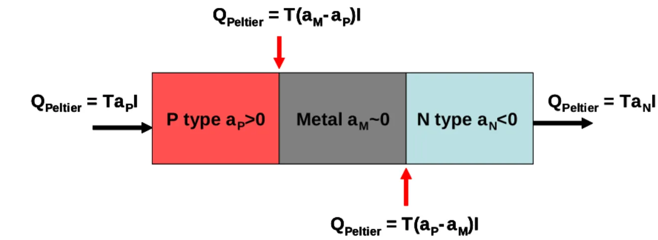
Heat is absorbed or released at the interface of two dissimilar materials by the

Peltier Effect, Fig. 1.3. When current is conducted across two similar materials, a heat

transfer will take place at the boundary due to the different Peltier coefficients of each

material. The Peltier heat term allows for thermoelectric refrigeration because heat can

be transferred in a direction opposite the temperature gradient by simply controlling the

current direction.

Q_Peltier= Ta_NI P type a_P>0 Metal a_M~0 N type a_N<0

Q_Peltier = Ta_PI

Q_Peltier = T(a_M- a_P)I

Q_Peltier= T(a_P- a_M)I

Q_Peltier= Ta_NI P type a_P>0 Metal a_M~0 N type a_N<0

Q_Peltier = Ta_PI

Q_Peltier = T(a_M- a_P)I

Q_Peltier= T(a_P- a_M)I P type a_P>0 Metal a_M~0 N type a_N<0 P type a_P>0 Metal a_M~0 N type a_N<0 Q_Peltier = Ta_PI

Q_Peltier = T(a_M- a_P)I

Q_Peltier= T(a_P- a_M)I

Figure 1.3: Peltier heat flow in a segmented material at uniform temperature. Heat transfer is localized at the interface where the Seebeck coefficient changes.

It is generally understood that heat flux is associated with entropy flux via

S

qT J . Dividing Eq. 1.1.6 by absolute temperature leads to

S

k

J

J

T

T













The above equation reconfirms that the Seebeck coefficient is actually the entropy

carried per particle.

Physically, charge carriers carry entropy proportional to the Seebeck coefficient.

The Seebeck coefficient is like a specific heat that when multiplied by temperature

determines the internal energy of the charge carrier. When an electron crosses an

interface it enters a different material system with different available electron energy

states. The entropy of the electron changes with the Seebeck coefficient and the

electron undergoes a heat transfer with the lattice. In principle this is an isothermal heat

transfer which occurs near the interface and is reversible with no entropy generation.

Advanced transport theory from the Boltzmann equation reveals that the actual interface

region has a thickness on the order of the mean free path of an electron and the

temperature of the lattice may not be uniform.

1.2 Governing Equation of Thermoelectricity

This section will derive the governing equation for thermoelectricity by using the

constitutive relation for heat flux from the last section. Later this equation will be used

to solve for the heat and work transfers on the boundaries of a thermoelectric device.

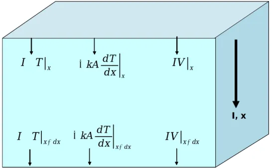
Energy is transferred in and out of the boundaries by three mechanisms: Peltier heat,

Fourier heat conduction, and electrochemical potential.

I, x x d T k A d x  x d x

I V

I



T

I V

I



T

I V

I



T

I V

I



T

Figure 1.4: Energy balance in a differential element of a thermoelectric material. From left to right: Peltier heat, Fourier heat conduction, electrical power

An energy balance is applied to the volume element and 1st order Taylor series

expansions performed on each term to give the following equation. 0 d T d dT dV J k J dx dx dx dx      _{ }    (1.2.1)

The change in voltage can be rewritten from Eq.1.1.5 to yield the following.

2 0 dT dT dT k JT J T dx dx T dx                (1.2.2)

The above equation is a 2nd order, non linear, PDE, and there are two methods to

solving it. One method is to make use of a similarity variable to transform it into a 1st

order, non linear ODE; this will be done in chapter 3. The second method which will be

temperature. This assumption is only valid over small temperature differences; chapter

3 will discuss the case when this assumption is not valid. Holding , ,k  constant we

can rewrite Eq.1.2.2 as the following [4].

2 2 2 0 d T k J dx    (1.2.3)

The above equation can be solved with 2 boundary conditions T _{x L} T_C and

0 H x

T _ T to solve for the temperature everywhere. The hot and cold side heat

transfers QH and QC have contributions from the Peltier heat and Fourier heat conduction,

Figure 1.4. The Fourier heat is found by solving for the temperature gradient at the

boundaries from Eq.1.2.3. The hot and cold side heat transfers are solved for below

2 2 i H H I R kA T Q I T L      (1.2.4) 2 2 i C C I R kA T Q I T L      (1.2.5)

where L is the total length of the material and Ri is the electrical resistance. The

generated electrical power is solved by subtracting QH from QC

2

E i

P I T I R

1.2.6 )

The equations for heat transfer have contributions from three terms: the first

term is the Peltier heat, the second term is the Fourier conduction heat, and the third

term is from a dissipative Joule heating process. Ideally, the Peltier heat term would

dominate in a good thermoelectric because the other terms are viewed as losses. The

Fourier conduction terms represents heat that is conducted by the temperature gradient

electrical work dissipating in the element which leads to unwanted heating in heat pump

mode, or electrical power loss in power conversion mode.

Thermoelectric power generation and refrigeration manifests by the

thermodynamically reversible Peltier heat transfers at the two interfaces. The bulk of

the material is needed only as a conduit for charge carriers to travel between the two

interfaces at high and low temperature. The other two properties k and ρ, represent

intrinsic losses in the conduit. The thermal conductivity represents an additional path

for heat to flow parallel to the heat carried by the electric current. The electrical

resistivity represents power dissipated by carrier transport.

1.3 Power Conversion and ZT

Now that the governing equation for thermoelectricity is built it can be applied to

a real device to solve for the energy conversion efficiency. A new property called the

figure of merit Z, will be defined which fully characterizes energy conversion efficiency.

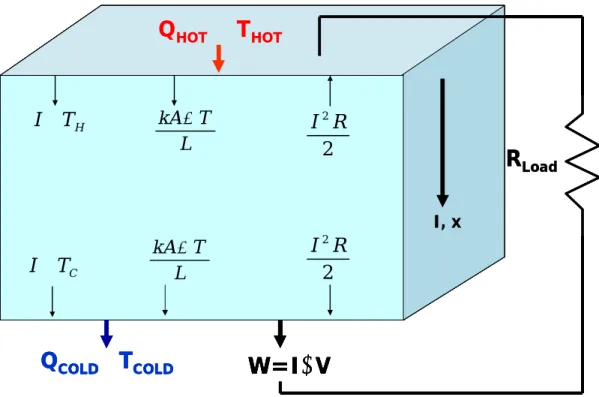
Consider a constant property, Thermoelectric (TE) material operating as a heat engine

with ends maintained at constant temperature and connected to an external load. The

TE element is referred to as a TE leg the current and heat transport is assumed to be one

dimensional and energy is conserved along the length (no heat loss at surface). The

ends are connected to an electrical resistor by perfect conductors with a Seebeck

coefficient equal to zero, so that thermoelectric effects in the leads are neglected. Each

boundary has three energy terms: the Peltier heat, Fourier conduction heat and a Joule

I, x k A T L  H I



T

Q

W=IΔV

Q

T

R



T

Q

W=IΔV

Q

T



T

Q

W=IΔV

Q

T



T

Q

W=IΔV

Q

T

R

Figure 1.5: Thermoelectric energy balance, constant properties

The conversion efficiency is equal to the electrical power dissipated in the load

resistance over the hot side power input.

2 2

2

P

I R

I R

kA T

Q

I T

L















Let us substitute in the resistance ratio M  R_L R_i where Ri is the internal

resistance of the TE leg and RL is the load resistance of the external circuit. The current

is rewritten as



1



T

I

R

M













1

1

1

1

2

T

M

T

ZT M

M





 

















_

_





   is the Carnot efficiency and

2

Z

k







properties called the figure of merit. Eq. 1.3.2 is a general equation for efficiency given

the boundary temperatures, the thermoelectric material properties and resistance ratio, M.

However to find the maximum efficiency we must use the relation d 0

dM 

 to find the

load matching condition corresponding to a maximum efficiency. Upon differentiating

Eq.1.3.2 with respect to M an optimal load matching condition and maximum efficiency

are found below

1

M





ZT

where T is the mean temperature and

2 T ZT k  

 is called the dimensionless figure of

merit. ZT is the most useful non-dimensional number the thermoelectric community

employs because this property alone determines the heat to electrical work conversion

efficiency. The commercial standard TE hasZT 1. A common assumption in device

will be looked at more closely in chapter 3. A similar treatment can be done for a TE

heat pump and will yield similar results for the importance of the figure of merit [2].

1.4 Semiconductors as Thermoelectrics

Good TE materials have a high figure of merit and therefore require a high

Seebeck coefficient, a high electrical conductivity, and a low thermal conductivity. This

is a very unusual combination of properties; for instance, usually good electrical

conductors like metals also have high thermal conductivity. While most thermally

insulating materials like plastics and ceramics are also electrically insulating. This

section will explain why semiconductor materials hold the greatest potential as TEs.

The three thermoelectric properties , ,k _{ are not independent, so it is hard to change}

only one property without changing the others. For example, increasing the number of

electrical carriers not only increases electrical conductivity but also increases thermal

conductivity, and decreases Seebeck coefficient. Both electrons and phonons (lattice

vibrations) contribute to the thermal conductivity of a material; the electron contribution

dominates in metals. The Seebeck coefficient is inversely proportional to carrier

concentration [7]. Fig. 1.6 illustrates each of three properties as a function of carrier

concentration. As the figure shows, metals have high electrical conductivities, but also

high thermal conductivities and low Seebeck coefficients. Insulators have high Seebeck

coefficients and potentially low thermal conductivities, but these properties are countered

by low electrical conductivities. The best thermoelectric materials which produce the

and carrier type can be easily changed with minimal affect to other properties, simply by

changing the doping type and doping concentration. With dopants, electrical

conductivity of semiconductors can reach up to the order of 105 S/m. The contribution

of electrons to thermal conductivity is not dominant for semiconductors, so a change in

doping concentration has a minor effect on thermal conductivity. Optimizing the doping

concentration is an important aspect of developing thermoelectric materials.

Figure 1.6: Thermoelectric properties S, σ ,k (Seebeck coefficient, electrical conductivity, thermal conductivity) as a function of carrier concentration. Semiconductors make the best thermoelectric materials.

1.5 State of the Art and Device Design

Thermoelectric devices operate as heat engines or heat pumps and are primarily

made from semiconductor materials. When the majority of electrical carriers are electrons,

negative values because direction of electron movement is opposite to that of the current.

On the other hand, when the majority of electrical carriers are holes, i.e., a p-type

semiconductor, the Seebeck coefficient and the Peltier coefficient have positive values.

Thermoelectric devices are made with pairs of p-type and n-type TE elements or “legs”.

A p-type leg is arranged electrically in series and thermally in parallel with an n-type leg

to form a “thermocouple couple”. Figure 1.7 shows a schematic of a typical

thermocouple running as a heat engine and as a heat pump.

Current by

diffusion N type P type

Cold Side Hot Side

electron holes

Current by

diffusion N type P type

Cold Side Hot Side

electrons holes

Current by

diffusion N type P type

Cold Side Hot Side

electron holes

Current by

diffusion N type P type

Cold Side Hot Side electrons holes N type P type N type P type Q N type P type N type P type Q Current by

diffusion N type P type

Cold Side Hot Side

electron holes

Current by

diffusion N type P type

Cold Side Hot Side

electrons holes

Current by

diffusion N type P type

Cold Side Hot Side

electron holes

Current by

diffusion N type P type

Cold Side Hot Side electrons holes N type P type N type P type Q N type P type N type P type Q

Figure 1.7 Schematic of thermoelectric devices: power generator (left) and thermoelectric cooler (right)

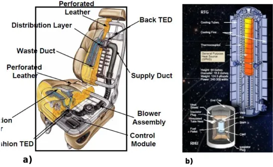
TE devices have been used in a several niche markets like small scale

refrigeration, and radioisotope generators. The most successful long term

implementation of TE devices has been in NASA’s deep-space spacecraft where

thermoelectrics have been used to generate power from a radioisotope (nuclear) fuel

source, Fig. 1.8b. When a spacecraft travels to the outer solar system, solar radiation is

too weak to be used as an energy source. In this case, the spacecraft’s electrical power

is generated by a thermoelectric heat engine operating between a hot nuclear fuel source

and cold space. One such RTG weighs about 55 kg and produces about 240 Watts of

graphite-encased plutonium heat source and the cold side radiates heat into space at 600

K. There is no ‘off’ switch: the radioisotope has a half-life of 87 years[8]. TE

refrigerators have recently been used in high-end automobile seats to deliver temperature

controlled air throughout the seats, Fig. 1.8a.

a)

a) b)b)

Figure 1.8: TE devices a) TE cooler in a car seat b) TE generator used in NASA space missions

Thermoelectric devices have several advantages in their design and operation:

1) No moving parts. Thermoelectrics are solid state materials with no moving

parts, no acoustic noise, and the material itself requires no maintenance. The

entire system design is greatly simplified over conventional cycles because

there is no working fluid and fewer components.

2) Reliability. TE materials are very stable when operated in the proper

temperature range. NASA has used TE generators in missions lasting for

decades and even in the harsh environment of space these generators have

3) Scalability. TE devices can be implemented in anything from integrated

circuits and MEMs to industrial sized waste heat recovery and can have high

power densities. TE devices are easily scalable over a huge range but are out

competed by other heat engine and refrigeration cycles at large scale.

4) Reversible. TE devices can be switched from power generation mode to

refrigeration mode simply by reversing the current, allowing for superior

temperature control.

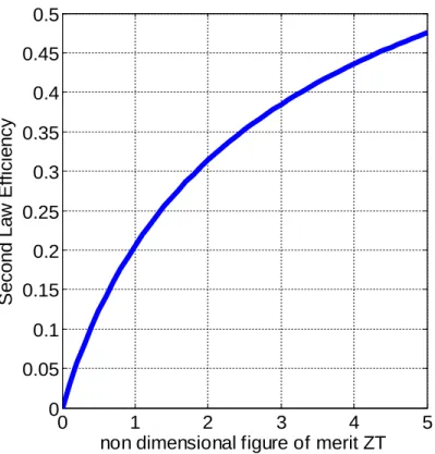
Fig. 1.9 plots the second law efficiency from Eq.1.3.4 versus ZT. It is believed that

TEs could begin replacing large scale refrigeration cycles at ZTs around 3-4

corresponding to second law efficiencies of 38-45%[2]. Thermoelectric generator

(TEG) second law efficiencies may never be directly competitive with traditional large

scale heat engines like steam and gas turbines that have second law efficiencies above

60%. However TEGs may play a large role in combined cycle applications where TEGs

operate at the hot side of an existing heat engine such as in a steam boiler or the cold

0 1 2 3 4 5 0 0.05 0.1 0.15 0.2 0.25 0.3 0.35 0.4 0.45 0.5

non dimensional figure of merit ZT

S e c o n d L a w E ff ic ie n c y

Figure 1.9: Second law efficiency (total efficiency divided by Carnot efficincy) vs. ZT for TH=500 K and

TC=300 K

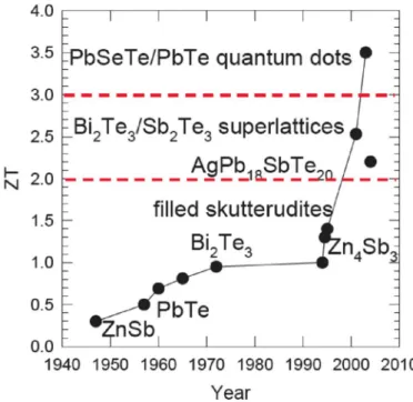
Over the last several decades the non-dimensional figure of merit has remained at

a maximum value of about unity. However, recent developments in nanostructured

thermoelectric materials have produced significantly higher figures of merit, Fig. 1.10.

Research at NASA-JPL, MIT-Lincoln Labs, Michigan State University, and other

organizations from about 1995 to the present has led to the discovery, characterization,

and laboratory-demonstration of a new generation of TE materials: skutterudites,

thin-film superlattice materials, quantum well materials, and PbAgSbTe (LAST)

compounds and their derivatives[1]. These materials have either demonstrated ZT of

~1.5-2 or shown great promise for higher ZT approaching 3 or 4. Quantum well materials

These materials make it possible to create TE systems that display higher ZT values than

those obtained in bulk materials because quantum well effects tend to accomplish two

important effects: 1) they tend to significantly increase density of states which increases

the Seebeck coefficient in these materials; and 2) they tend to de-couple the electrical and

thermal conductivity allowing quantum well materials to exhibit low thermal

conductivities without a corresponding decrease in electrical conductivity. The LAST

compounds have shown embedded nanostructures within the crystal matrix that may

exhibit quantum well effects[1].

Figure 1.10: Timeline of ZT over the past 60 years

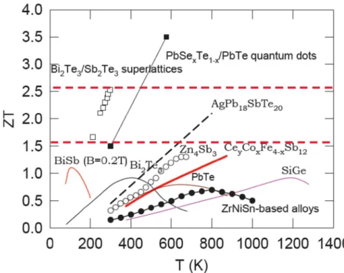
TE materials have temperature dependant properties and temperature dependant

ZT values. Each material has a finite operating temperature range around the maximum ZT value which means if a device is to operate over a large temperature range then more

than one material system must be employed. Fig. 1.11 plots the temperature dependant

Figure 1.11: ZT vs. temperature for different material systems. Bi2Te3 is the most common room

temperature TE

Although there are many reports of nano-featured TE materials with high ZTs few

of these materials can be fabricated economically or in sufficient quantities. Bi2Te3 is

the best bulk thermoelectric around room temperature and is the only commercially

available TE. Bi2Te3 has been widely used in small scale refrigeration for decades and

has recently been seriously considered for power generation. Researchers have taken a

renewed interesting in thermoelectric power generation in light of pressing issues of

energy and environment the world faces in the 21st century. The challenge is to create a

TE material that is economical and scalable to large systems in order to improve energy

efficiency and energy conservation.

In the next chapter a high ZT nanocomposite will be introduced. The purpose of

the following work is to develop a power conversion measurement system in order to test

designed to measure conversion efficiency under the same conditions of a real

thermoelectric generator. A temperature dependant model will be used to compare the

Chapter 2: Bi

Te

Nanocomposite

The Bi2Te3 material system is the only commercially available TE material and

one of the most well studied. The ZT for this alloy is around 1 at room temperature

which makes it very attractive for refrigeration and waste heat recovery applications.

Bi2Te3 was thus the logical choice of material systems to implement a novel

nanocomposite approach on. This chapter will describe the synthesis and individual

property measurements of the Bi2Te3 P-type nanocomposite. This work represents a

collaborative effort between Dr. Chen’s group at MIT and Dr. Ren’s group at BC. The

results where recently published in [9].

2.1 P-type Bi

Te

nanocomposite

The dimensionless thermoelectric figure-of-merit (ZT) in bulk bismuth antimony

telluride alloys has remained around 1 for more than 50 years. We’ve shown that a peak

ZT of 1.4 at 100°C can be achieved in p-type nanocrystalline bismuth antimony telluride

bulk alloy. These nanocrystalline bulk materials were made by hot pressing

nanopowders ball-milled from crystalline ingots under inert conditions. Thermoelectric

property measurements and microstructure studies that the ZT improvement is the result

of low thermal conductivity caused by increased phonon scattering by grain boundaries

and defects. This nanocomposite approach may allow the development of high

performance bulk thermoelectric materials at low cost.

In the past researchers have successfully increased ZT in superlattices due to a

reduced thermal conductivity [10,11]. The nanocomposite approach uses the same

randomly oriented way. The nanoscale grains effectively increase phonon scattering

without adversely affecting the Seebeck coefficient and electrical conductivity. As

opposed to thin films the P-type Bi2Te3 nanocomposite bulk properties are nearly

isotropic. Other thin film methods grow the material layer by layer, which is a very

slow and expensive process. The nanocomposite method is based on ball milling and

hot-pressing of nanoparticles into bulk ingots. This approach is simple, cost effective, and

can be applied to other materials.

It is known that hot pressed TE material can be readily made into segmented legs

where more than one TE material is stacked in series [ 12 ]. In this way the

nanocomposite can be easily used in high temperature power generation applications

where segmented legs are employed. Nanocomposites do not suffer from the cleavage

problem that is common in traditional zone-melting made ingots, which leads to easier

device fabrication and system integration, and a potentially longer device lifetime [9].

2.2 Sample Preparation

All nanocomposite samples were fabricated at Boston College (BC).

Nanopowders were prepared by ball milling bulk p-type BiSbTe alloy ingots [13]. Bulk

disk samples of 1¼ to 2½ cm in diameter and 2 to 15 mm thick were made by

hot-pressing the nanopowders loaded in 1¼ to 2½ cm (inner diameter) graphite dies[13].

Disks of 1¼ cm (diameter) and 2 mm thick, and bars of about 2 mm by 2 mm by 12 mm,

were cut from both the axial and disk plane directions. The disks and bars were also

polished for electrical and thermal conductivity and for Seebeck coefficient

To achieve high ZT, control of the size and quality of the starting nanoparticles is

essential. TEM images of the ball-milled powder show that the particle size is between

5 and 50 nm with a mean of about 20 nm (Fig. 2.1 C and D). Detailed microstructure

studies by BC show that in general, most of the grains are nanosized (Fig. 2.1 A and B).

Furthermore, these nanograins are highly crystalline, completely random (large angles

between adjacent lattice planes) and have very clean boundaries between grains.

Figure 2.1: A and B) TEM images of nanograins after hot pressing C) TEM image after ball milling D) TEM image after ball milling [9]

2.3 Property Measurement Methods

Thermoelectric properties are difficult to measure accurately. Often they are

measured independently of each other on different machines using different samples.

Combined experimental error from the three measurements can easily dominate the

results.

All of these measurements were confirmed by two independent techniques at both

BC and MIT on more than 100 samples. The electrical conductivity was measured by a

four-point current switching technique. The Seebeck coefficient was measured by a static

DC method based on the slope of a voltage versus temperature-difference curve, using

commercial equipment [14] on the same bar-type sample with a dimension of 2 mm by 2

mm in cross-section and 12 mm in length.

The thermal diffusivity α, was measured by a laserflash method on a disk using a

commercial system [15]. Thermal conductivity was calculated using the equation k = α ρ

cp, where ρ is the density and cp is the specific heat of the material which was measured

using a differential scanning calorimeter [15].

2.4 Individual Property Data

Our nanocomposite properties were measured as a function of temperature by

MIT and BC. Fig. 2.2 shows all the properties as a function of temperature including

250 300 350 400 450 500 550 0.8 1 1.2 1.4 1.6 1.8 2 2.2x 10 -5 Hot Temperature E le c tr ic a l R e s is ti v it y 250 300 350 400 450 500 550 0.9 1 1.1 1.2 1.3 1.4 Hot Temperature T h er m al c onduc ti v it y 250 300 350 400 450 500 550 1.9 1.95 2 2.05 2.1 2.15 2.2x 10 -4 Hot Temperature S e e b e c k c o e ff ic ie n t 300 350 400 450 500 550 0.7 0.8 0.9 1 1.1 1.2 1.3 1.4 Hot Temperature Z T

Figure 2.2: Temperature dependant properties P-type Bi2Te3 nanocomposite, from upper left going

clockwise: electrical resistivity, thermal conductivity, ZT, Seebeck coefficient [9]. The red triangles are from experimental data and the blue curves are from a best fit polynomial.

Below is a table of the estimated uncertainty in each of our property

measurements and the resulting average Gaussian uncertainty in ZT.

Table 1: Instrument uncertainty in individual property measurements

Property Instrument uncertainty

Seebeck Coefficient 5%

Electrical Resistivity 5%

Thermal Conductivity 8%

ZT 11.7%

An increase in ZT of 12% is significant; therefore it is undesirable to have an

uncertainty of 12% in our measurement. The most convincing way to verify our high

conclusive tests because they essentially verify all the properties simultaneously. My

lab mates Qing Hao and Austin Minnich performed a maximum ΔT cooling measurement

while I designed and performed a novel power conversion measurement (Chapter 4).

The energy conversion measurement system is designed to measure efficiency rather than

ZT as a function of temperature; in fact ZT is only an indicator of performance because it

is based on the constant properties model. Therefore it was necessary to use a

temperature dependant model to predict conversion efficiency and verify our measured

Chapter 3: Modeling Based On Temperature

Dependent Properties

Thermoelectric properties are highly temperature dependent and every real

material has an operating range around its peak ZT value (Fig. 1.11). If a device is to

operate over a large temperature range then more than one material system must be used.

An efficiency model is needed that captures the temperature-temperature of the properties

in different materials. Although ZT is the best non-dimensional number the

thermoelectric community has it is derived from the constant properties model and cannot

precisely predict device performance over large temperature differences. In the case of

our nanocomposite it would be very unclear what ZT values to use since the properties

may vary by a factor of 2 over the operating range (Fig. 2.2). This section will introduce a

temperature dependent model used to predict power conversion efficiency.

3.1 Temperature Dependant Conversion Efficiency

The Bi2Te3 nanocomposite properties,



   

T

,



T

,



 

T

function of temperature so the typical ZT efficiency Eq. 1.3.4 is not applicable. For

this reason it is necessary to go back to the governing equation for thermoelectricity (Eq.

1.2.2) and keep the temperature dependence of the electrical resistivity, thermal

conductivity and Seebeck coefficient. The following is a similarity solution to the

governing equation of thermoelectricity, [2]

dY

d

T

dT

dT

Y





 



where Y T

_{ }

 

Eq. 3.1.1 is a 1st order, nonlinear ODE, which can be solved for numerically with

one boundary condition, Y T J





current density. This equation is solved by holding T_C constant to represent the cold side reservoir and sweeping the boundary condition Y T J





 

to a different current density condition because T_C is kept constant. In this way





Y T J has determined Y T

 

1 H C T T dT J L Y  

_





 

 









1

1

Y T

T

T

Q

Q

Y T

T

T









 

 



Alternatively the efficiency and heat transfers can be computed by a finite

difference solution [16,17]. In this method the TE leg is subdivided into many small

segments such that there is a small temperature difference across each segment and

in [2], and should yield that same results given a sufficient number of segments is used.

The finite difference model is more attractive when considering a segmented leg (more

than one material stacked in series).

The quantities defined in 3.1.3, 3.1.4 and 3.1.5 are important quantities that must

be measured experimentally. The graphs to be generated experimentally will be

efficiency versus current or load matching, and maximum efficiency versus temperature

difference. The maximum efficiency is determined by finding the Y T J

_

_

maximum efficiency vs. delta T for T_C 300[ ]K . The temperature dependant curve is generated from Eq.3.1.5 given TH and TC. The temperature independent curve was

generated by fitting Eq.1.3.4 to the temperature dependant model data corresponding

Nanocomposite Efficiency vs. Delta T

Figure 3.1: Maximum efficiency vs. ∆T for the temperature dependant model and a best fit ZT=1.27 model. Property data from previous section

In order to generate Fig. 3.1 the load matching condition which produces the

maximum efficiency at a given temperature difference must be found. Figure 3.2 plots

efficiency vs. resistance ratio, M for both models (equations 1.3.2 and 3.1.4).

Interestingly the peak efficiency occurs at nearly the same load matching and the curves

are very similar except for an offset between them. The model results in the last two

Efficiency vs. Rratiol (Fixed Delta T) 0.075 0.08 0.085 0.09 0.095 0.1 0.5 1 1.5 2 2.5 Rload/Rinternal E ff ic ie n c y T dependant ZT=1.27

Figure 3.2: Efficiency vs. load matching for both temperature dependant and independent models. Tc=300°K, TH=500°K

There are two conclusions to be drawn from the last two graphs:

1) The temperature-dependent model is necessary to precisely verify thermoelectric

properties over a large temperature range. For a material still under

development where different techniques are being applied to enhance properties,

the temperature-dependent model should be used to resolve these differences. If

a TE the material is to be used in a high performance application like the

aerospace industry then most likely a temperature-dependent model will be

necessary.

2) The constant ZT model is accurate enough for preliminary engineering of

feasibility study or if the application doesn’t have very stringent constraints on

performance, then an effective ZT model can be used.

In general, it is recommended to first use the temperature-dependent solution if

the property data is available, since this method is not computationally expensive for a

single leg. Next an effective ZT should be fit to the efficiency solution over the range of

interest and the effective or average property values calculated. The

temperature-dependent solution should be compared to the temperature-independent

solution so uncertainty estimates can be calculated and then a decision can be made on

which model to use. If property data is very limited then the constant properties model

Chapter 4: 1

Generation Efficiency Testing

The previous chapters have demonstrated that thermoelectric properties are highly

temperature dependant and difficult to measure accurately. Since errors in individual

property measurements compound to give larger error in power efficiency we decided to

measure the power efficiency directly in order to characterize our material better. A

power conversion measurement system was developed to better characterize our TE

material by testing it under the same conditions as a real device. This system measures

the performance of a TE material in the most direct way and will be used to evaluate the

properties simultaneously as well as individually. Finally I will compare the

experimental results with the model results from the property data in chapter 3.

I, x

T

Q

W=IΔV

Q

T

R

Q

T

Q

W=IΔV

Q

T

R

T

Q

W=IΔV

Q

T

T

Q

W=IΔV

Q

T

R

Q

A power conversion measurement like this one requires all the elements of a real

working device. The material must be in good thermal contact with a heat source and

sink and must be electrically connected to an external circuit where the electrical power is

dissipated, Fig. 4.1. Similar to a commercial TE module the leg needs to be soldered to

electrical leads which are also good electrical conductors if a TE material is to be made

into a device. The biggest different between a TE material and a device ready TE leg is

a metalized layer on the ends that can be easily soldered to. The metalized layer is

usually Ni and its purpose is to allow soldering with low electrical and thermal

resistances and to act as a diffusion barrier to solder contamination. Since the material

is a doped semiconductor the danger is that solder will diffuse into the sample and

effectively dope it, and change the properties.

In the case of the nanocomposite a 12.5 µm thick Ni foil layer is attached to either

end during hot pressing, Fig. 4.2 is a picture of a nanocomposite sample with Ni foil

contacts. There is always an electrical contact resistance between the Ni layer and TE

material, as well as a smaller thermal contact resistance. A thermal contact resistance

will cause a temperature drop across the interface and decrease the maximum allowable

Carnot efficiency. Electrical contact resistance decreases power output because there is

a voltage drop across the interface and electrical power is dissipated as Joule heating.

The presence of electrical contact resistance is an important distinction between a bare

TE material and a device ready leg, the effects on overall performance will be seen later

in the chapter.

Figure 4.2: Nanocomposite sample (1.5mm each side) with 12.5µm Nickel foil on the top and bottom of the sample. The Ni layer allows for soldering while acting as a diffusion barrier to solder contamination.

The 1st generation of the power conversion measurement system was designed to

measure the current flowing through the sample, the voltage across the sample as well as

the cold side heat flux and temperatures. From these measurements one can solve for

the conversion efficiency using

TE TE H C TE IV IV Q Q IV       (4.0.1)

where I is the current, VTE is the voltage across the sample/load resistance and QC is the

cold side heat transfer measured by a heat flux sensor. In principle the measurement is

simply performing an energy balance over the TE leg, in practice obtaining an accurate

measurement of the above quantities can be challenging for the following reasons:

1) One should be careful when measuring QH or QC because the presence of

unwanted modes of heat transfer can create a difference in heat transfer measured

at the sensor to the actual heat transfer entering or exiting the sample. The heat

Air conduction and radiation occur at the heater, leg side walls, and heat flux

sensor. When measuring a single leg it is easier to accurately measure the heat

flux at the cold side rather than at the hot side because the temperature is closer to

ambient and therefore thermal losses are lower. The presence of heat loss along

the side walls of the sample suggests that a cold side heat flux measurement leads

to an upper limit estimate for efficiency while a hot side heat flux measurement

leads to a lower limit estimate for efficiency.

2) The thermovoltages and the electrical resistances of the sample are small which

can lead to relatively large uncertainties in voltage if a high precision instrument

is not used. Thermo-electrical voltage resolution on the order of 10µV is

commonly needed in such experiments. A National Instruments SCXI

conditioning box was used to measure all the voltages (<1 µV resolution) and

thermocouples (<0.05°C resolution, ~.1°C accuracy). Precautions were also

taken to reduce the RF noise in the electrical system such as shielding and

soldered connections. The cryostat pressure vessel is made from aluminum

construction and acts to shield the circuits inside from external noise, no AC

currents where run inside the vessel, and shielded wires were used when ever

possible outside the vessel. A type-K thermocouple wire feed thru was installed

so that the thermocouple circuit was made entirely of thermocouple wire with no

change in material. Originally the cryostat had a copper feed through that

thermocouples wires were soldered to, this can give erroneous results due to a

3) Variation in sample properties and contact resistance are always present which

make it hard to distinguish experimental error from an actual change in expected

properties. For example, the hot pressed Ni foil sample electrical resistance can

varying substantially depending on the hot pressing conditions. Attaching a Ni

foil layer to the Bi2Te3 material with good mechanical strength and low electrical

resistance presents significant challenges and it is a topic of ongoing research [9].

Many times during our experiments the Ni layer would detach during soldering

making an efficiency measurement impossible or the contact resistance was found

to be too high leading to poor efficiency. Additionally, the samples where cut

into blocks and sometimes these blocks varied in cross section along its length

which can lead to large uncertainties in the geometry.

4.1 Power Conversion Measurement System Design

The 1st generation power conversion measurement system was designed to

measure the current, voltage across the sample and cold side heat flux and temperatures

to solve for conversion efficiency by Eq. 4.0.1. A photo of the system with a sample

mounted is shown in Fig. 4.3. A copper wire is soldered to the top of the sample which

is maintained at T and conducts both the current and heat from the heater. A _H

thermocouple soldered to the top of the sample measures T and acts as one of the two H

voltage probes. The bottom of the sample is soldered to a copper heat spreader

maintained at T . Mounted to the heat spreader is a cold side copper wire to complete _C

the electrical circuit and a thermocouple which measures T and acts as the second _C

measures Q conducted across it. The heat sink for the heat flux sensor is the cryostat _C

cold finger which is maintained lower than room temperature by chilled coolant (water

and antifreeze) pumped through the cold finger. The electrical load resistance is

controlled by two power MOSFETs[ 18 ]. A schematic representation of the

thermo-electrical energy flow is given in Figure 4.4 where the heat transfers are depicted

by red arrows and the electrical power is in green. Ideally there is no energy loss along

the side walls of the leg and all the cold side heat is conducted across the heat flux sensor.

Notice the heat loss from the surfaces and heat conduction loss and Joule heating and

from the cold side electrical wire.

Heater

Load Resistance

Heater

Load Resistance

Radiation Shield

Heat Flux Sensor

Copper Spreader T=25-30C

Q_HOT

QCOLD MEASURE

Copper Base

Pvacuum~ 5e-5 Torr

Load Resistor Q_Radiation I QCOLD Q_{Loss Conduction} Q_{Air Conduction} Heater QJoule Radiation Shield

Heat Flux Sensor

Copper Spreader T=25-30C

Q_HOT

QCOLD MEASURE

Copper Base

Pvacuum~ 5e-5 Torr

Load Resistor Q_Radiation I QCOLD Q_{Loss Conduction} Q_{Air Conduction} Heater

Heat Flux Sensor

Copper Spreader T=25-30C

Q_HOT

QCOLD MEASURE

Copper Base

Pvacuum~ 5e-5 Torr

Load Resistor Q_Radiation I QCOLD Q_{Loss Conduction} Q_{Air Conduction} Heater QJoule

Figure 4.4: Schematic of energy flow within the system. The red arrows are heat transfers and the green arrows are energy flows from the electrical circuit.

The tests where conducted in a cryostat under a high vacuum (5x10-5 torr) to

eliminate convection and reduce air conduction loss Fig. 4.5. In order to achieve lower

pressure the chamber was modified so that the pump was connected to the bottom with a

pressure gauge very close to the sample. Originally the pump was connected to a needle

valve at the top of the chamber so there was a big pressure drop across that valve and

down to the bottom of the chamber. Instead the valve was bypassed by attaching a

custom made flange to a window at the bottom of the chamber near the sample. There is

essentially no pressure drop from the bellow to the sample because there is no flow

restriction. The pressure gauge was also moved from the turbo pump inlet to a location