Advances in data-driven models for transportation

(1)

Advances in Data-Driven Models for Transportation

by

Yee Sian Ng

Submitted to the Sloan School of Management

in partial fulfillment of the requirements for the degree of

Doctor of Philosophy in Operations Research

at the

MASSACHUSETTS INSTITUTE OF TECHNOLOGY

June 2019

c

○ Massachusetts Institute of Technology 2019. All rights reserved.

Author . . . .

Sloan School of Management

May 17, 2019

Certified by . . . .

Dimitris Bertsimas

Boeing Professor of Operations Research

Co-Director, Operations Research Center

Thesis Supervisor

Accepted by . . . .

Patrick Jaillet

Dugald C. Jackson Professor of Electrical Engineering

and Computer Science

Co-Director, Operations Reserach Center

(2)

(3)

Advances in Data-Driven Models for Transportation

by

Yee Sian Ng

Submitted to the Sloan School of Management on May 17, 2019, in partial fulfillment of the

requirements for the degree of

Doctor of Philosophy in Operations Research

Abstract

With the rising popularity of ride-sharing and alternative modes of transportation, there has been a renewed interest in transit planning to improve service quality and stem declining ridership. However, it often takes months of manual planning for operators to redesign and reschedule services in response to changing needs. To this end, we provide four models of transportation planning that are based on data and driven by optimization. A key aspect is the ability to provide certificates of optimality, while being practical in generating high-quality solutions in a short amount of time. We provide approaches to combinatorial problems in transit planning that scales up to city-sized networks. In transit network design, current tractable approaches only consider edges that exist, resulting in proposals that are closely tethered to the original network. We allow new transit links to be proposed and account for commuters transferring between different services. In integrated transit scheduling, we provide a way for transit providers to synchronize the timing of services in multi-modal networks while ensuring regularity in the timetables of the individual services. This is made possible by taking the characteristics of transit demand patterns into account when designing tractable formulations.

We also advance the state of the art in demand models for transportation opti-mization. In emergency medical services, we provide data-driven formulations that outperforms their probabilistic counterparts in ensuring coverage. This is achieved by replacing independence assumptions in probabilistic models and capturing the in-teractions of services in overlapping regions. In transit planning, we provide a unified framework that allows us to optimize frequencies and prices jointly in transit networks for minimizing total waiting time.

Thesis Supervisor: Dimitris Bertsimas

Title: Boeing Professor of Operations Research Co-Director, Operations Research Center

(4)

(5)

Acknowledgments

I wish to thank my thesis committee, Dimitris Bertsimas, Patrick Jaillet and Carolina Osorio for their time, suggestions and valuable comments. This thesis also benefitted from the support of our collaborators from Mitsubishi and MELCO, Yoneta, Ryuya, Arvind and Daniel.

This thesis was written over five years of guidance under Dimitris, who has an unerring taste for practical insights from our research together. He has an inspiring amount of enthusiasm for and optimism in the value of research, and taught me that our work is not complete until it can be understood and used by others.

My collaboration with Julia Yan has been crucial to the success of this thesis. Her use of simple examples has saved us from the blind spots of my algorithmic tendencies on multiple occasions, and her creativeness in solution approaches is inspiring.

I am deeply grateful to Melvyn and Patrick who supported and believed in me when I began research in the Future Urban Mobility Lab under the Singapore-MIT Alliance. I spent a summer under the tutelage of Melvyn, who sat me down to work through basic proofs on the board in his office together – I can only hope to pay his generosity and patience forward.

My time at the Operations Research Center (ORC) is a memorable one. I wish to thank Miles, Iain and Joey for inspiring me to contribute and be part of open-source communities. Alex, Angie, Chongyang, Daniel, Mila, Nataly, Nikita, Joel, Will and many wonderful seniors have made the ORC warm and welcoming. My batch mates are a great source of help and companionship: Max Biggs, Max Burg, Rim, Ilias, Lauren, Kevin, Konstantina, Michael, Lennart, Jing, Matthieu. Many thanks to Bart, Bartolomeo, Chris, Daniel, Hari, Martin and Sebastien for their time in discussing research ideas with me. I also wish to thank Agni, Andrew, Arthur, Chris Coey, Deeksha, Elisabeth, Emily, Emma, Galit, Holly, Jackie, Jess, Joshua, Jourdain, Julia, Kayla, Lea, Matthew, Or Dan, Peter, Qingyang, Rebecca, Ryan, Sam, Sean, Susan, Tamar, Ted, Vasileios, Yuchen and Zach for their great company. One of the most important periods for me was doing an internship in the T-4

(6)

divi-sion with the Center for Nonlinear Studies in Los Alamos. Line is an amazing source of support and encouragement who helped me through some of my most difficult pe-riods. Sidhant is a wonderful mentor who pushed me to think beyond “linear decision rules” for optimization. I also had the good company of Andrey, Arun, Carleton, Deep, Harsha, Kaarthik, Kalina, Marc, Misha, Russell, Scott, Tillmann Mühlpfordt and Tillmann Weisser over a summer of food and sun and sand.

I spent an equally amazing summer in Google with Ross as my host. Apart from being great company, he provided the guidance I needed while entrusting me with autonomy. Which I spent on rock-climbing and doing dubious things with Jonathan and Michelle, in the company of fellow interns Andrew Ross, Felix, Harini, Jisoo, Kevin, Samantha, Zack and Zelda. Together with Miles, Ondrej, Christian, Jon and the rest of the O.R. team, they have made my decision to join Google an easy one.

Special thanks goes to Jack and Jenny for making Cambridge feel like home, and reminding me that how we spend our days is how we spend our lives. They have filled mine with music and food and obscene amounts of television and movies. Thanks to Daisy and Chester and Marcos for being like family – their sense of fun and humour is expansive and infectious, and their company is deep and nourishing. Thanks to Colin for being a wonderful drinking buddy and to Sarah for her brownies.

Many other people have been important to me at various points, and I wish to acknowledge them: Yossiri, Saurabh, Dax, Gladia, Grace Fong, Grace Goon, Grace Yeo, Bingshao, Sanqian, Haiwen, Charlotte, Delph, Danny, Jaren, Alvin, Mingfang, Gargoei, Gao Yuan, Rachel, Sau Ling, Li Cui, Cedric, Shawn, Beng, Kelly, Kenneth, Krishnan, Cynthia, Weiyi, Christine, Qinying, Yangshun, Isabelle, Chloe, Shujing, Ally, Louise, Jiahao, Martijn, Carolyn, Frans and Frank.

Last but not least, I wish to thank my family for their love and support. My parents Thomas and Mary have deeply imprinted on me the value of a good education and the importance of being a good person. My siblings are a great source of counsel, and I look forward to experience and celebrate life in all its stages with them.

(7)

List of Figures

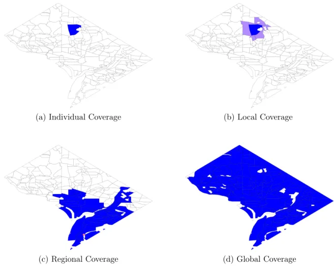
2-1 Different hierarchies of coverage for Washington D.C. Illustrates the geographical regions corresponding to (a) individual regions, (b) each region with those adjacent to it, (c) drivetime coverages from each station, and (d) the whole of Washington D.C. . . 39 2-2 Average hourly number of emergency calls per region. This is based on

data of emergency calls requiring ambulatory care for DCFEMS, from Jan 2012 to Mar 2013. . . 43 2-3 Sample drivetime region. The orange dots corresponds to road nodes

reached within 10minutes, based on drivetimes using OpenStreetMap data, starting from the fire station (red dot). The grey areas indicate the coverage regions, corresponding to those that contains at least 1 orange dot. . . 44 2-4 Deployment Coverages for the Robust and Stochastic deployment

mod-els with 35 ambulances. The regions are shaded by counting the num-ber of ambulances available within 10minutes. The size of the orange circles corresponds to the number of ambulances allocated to that lo-cation. . . 49

3-1 A screenshot of Google Maps illustrating route options in Japanese transit. (Accessed 2017-11-03) . . . 59 3-2 A map of the Kanagawa trains network. . . 72

(12)

3-3 Optimization progress for multiple different random starting points and two example budgets, on the full Kanagawa network and using frequency-setting and line pricing. Each line corresponds to the objec-tive function value from a different random starting point. . . 76 3-4 Optimal objective values under frequency-setting without pricing,

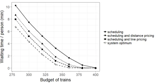
co-ordinated setting and distance pricing, coco-ordinated frequency-setting and line pricing, and the system optimum. The network of study was the full Kanagawa network. . . 77 3-5 Distribution of utilities among passengers for two different

frequency-setting and pricing policies on the full Kanagawa network. Note that because passengers lose time and money while commuting, all utilities are negative. . . 78 3-6 Proportion of Kanagawa commuters who would choose line-pricing

in-stead of distance-pricing, by travel distance. . . 79 3-7 A subset of the MBTA network used in Section 3.5.2, showing parts of

the Red, Green, Orange, and 1 bus (gray) lines. Stations further out-side of the metropolitan core of the network, and some 1 bus stations, are omitted for clarity. To generate more route options for commuters, some stations that were within a 0.5 mile walk of each other were as-sumed to be substitutable for each other. Stations that were viewed as substitutable are surrounded with dotted boxes. . . 80

4-1 An illustration of transfers excessive travel times due to transfers. . . 103 4-2 Synthetic bus network generated under the direct-route model without

travel time constraints. The network above was produced using the direct-route column generation procedure without edge preprocessing, with budget 𝐵 = 24. A single line is produced connecting all of the stops. . . 108

(13)

4-3 Synthetic bus network generated under the direct-route model with travel time constraints. The network above was produced using the direct-route column generation procedure without edge preprocessing, with budget 𝐵 = 24. . . 109 4-4 Synthetic bus network with single-transfer column-and-constraint

gen-eration and travel time constraints. We illustrate the network produced in each iteration of the single-transfer column-and-constraint genera-tion procedure. The budget was set to 𝐵 = 1.5, which is exactly the budget needed to sustain a grid network. . . 110 4-5 Optimization lower and upper bounds for an iteration of the full

sub-problem. The bounds are based on a 𝑁 = 40 random network. Because the subproblem is a maximization problem, the lower bound represents the actual solution values. . . 113 4-6 Boston-area bus networks generated from the MBTA demand matrix.

Blue lines represent the original network, red lines represent bus lines that were generated by the algorithm, and green lines represent the final optimized bus network. . . 117 4-7 Boston-area bus networks generated from the Blue Bikes demand

ma-trix. Blue lines represent the original network, red lines represent bus lines that were generated by the algorithm, and green lines represent the final optimized bus network. . . 118

5-1 The MBTA subway network. . . 139 5-2 Coordination of Timetables. We built visualizations of Marey

dia-grams [116] to illustrate the schedules and occupancies of the different services. The lines are colored based on the services that they corre-spond to, and their width correcorre-sponds to the occupancy along each service run. This is an illustration of the best found schedule for the MBTA in-bound red and orange subway network. . . 140

(14)

5-3 Comparison of the Model Runtimes. We ran the Network, Connect, Segment and Arrival formulations on two different networks with a time limit of 10,000 seconds and MIPFocus=3. For each, we plot the incumbent solutions based on their objective value under the network formulation and the corresponding time they were generated. We also plot lower bounds (in orange) on the optimal objective value as time proceeds. . . 142

5-4 Computational runtimes with regularity constraints. We ran the Net-work, Connect, Segment and Arrival Model with regularity constraints on inbound red and orange lines with a time limit of 10,000s and MIPFocus=3. For each, we plot the incumbent solutions based on their objective value under the network formulation and the corresponding time they were generated. We also plot lower bounds (in orange) on the optimal objective value as time proceeds. Finally, we added points to show the MIP start solutions of the Network Model before it started the branch-and-bound process. . . 143

5-5 Computational runtimes for the Late Night T network. We ran the Connect Model (in blue) and Arrival Model (in purple) models on the full MBTA network including both buses and trains. For each, we plot the incumbent solutions based on their objective value under the connect formulation and the corresponding time they were generated. We also plot the best bounds (in orange) on the optimal objective value as time proceeds. . . 146

A-1 Scenarios generated by the C&CG algorithm. This is based on the ro-bust deployment model for 35 ambulances, with parameter 𝛼 = 0.01. We illustrate the first 16 scenarios generated as chloropleths, and cor-responding deployment plans as orange circles, from left to right, top to bottom. . . 152

(15)

C-1 Some suggestions for the MBTA Late Night T. Both images taken from https://www.mbta.com/schedules/. Map data c○2019 Google. . . . 161 C-2 Recommended Late Night Services for the MBTA Network. A map

of the recommended MBTA services based on optimization using the Late Night T data. All the subway lines (red, blue, orange and green) are maintained. Among the bus services, the ones that are maintained are plotted in purple, and the ones to be left out of late night services are plotted in grey. Map tiles by Stamen Design, under CC By 3.0. Data by OpenStreetMap, under CC BY SA. . . 162

(16)

(17)

List of Tables

2.1 Summary of the Notation . . . 32 3.1 Summary of the Notation . . . 58 3.2 Travel times for various origin-destination pairs on the Kanagawa network 72 3.3 Frequency-setting on a small network under varying budgets and

com-muter sensitivities to congestion. . . 74 3.4 Price-setting on a small network under varying budgets and commuter

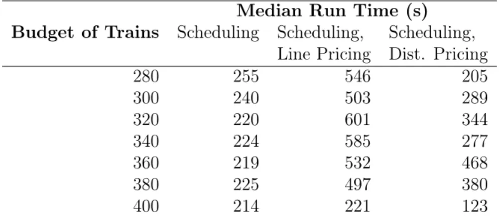
sensitivities to congestion . . . 75 3.5 Median run time over thirty iterations for various budgets. . . 76 3.6 Optimal objective values under the system optimum, frequency-setting

without pricing, coordinated frequency-setting and line pricing, and coordinated frequency-setting and distance pricing. The network of study was the Boston network. . . 81 4.1 Summary of the Notation . . . 87 4.2 Performance of preprocessed subproblem as compared to the full

sub-problem. We compared both approaches in performance and compu-tation time (the full subproblem was capped at 48 hours). Each row of the table represents 25 different simulations. . . 112 4.3 Objectives of the original MBTA network and the optimized network 115 4.4 Characteristics of the original MBTA network and the optimized network116 4.5 Running time for Algorithm 2 on the Boston dataset . . . 118 5.1 Summary of the Notation. . . 126

(18)

5.2 Overview of the four scheduling formulations. . . 135 5.3 Computational Performance on the Red and Orange Lines. We ran all

the models on the inbound red and orange lines with a time limit of 10,000 seconds, and keep track of the number of the top three classes of cuts generated. All but the Network Model terminated at optimal-ity. We report the MIP Gap for each of them, defined as the lower and upper objective bound divided by the absolute value of the upper bound. We also report the time when the Network Model found a better schedule (if applicable). . . 141 5.4 Computational Performance on the Full Subway Network. We ran the

models on the full MBTA subway network with a time limit of 10,000 seconds, and keep track of the number of the top three classes of cuts generated. All but the Connect Model terminated at optimality. . . 141

A.1 Robust Deployment Plans. Generated for different parameter values 𝛼, with varying numbers of ambulances. For values of 𝛼 above 0.01, the model saturated quickly which resulted in deployment plans that were not as competitive. . . 153 A.2 Deployment Plans. Generated for each model with varying numbers

of ambulances. Both the Stochastic and Robust formulations evenly distribute the allocation of ambulances, but the MEXCLP and MALP clusters them in a few central locations. . . 154 A.3 Coverage Peak Steady. Simulated coverages based on 12 replications,

each for 360 hours of continuous peak-hour ambulance operations, with steady turnaround times. Shaded cells are results that should be ignored.155 A.4 Coverage Peak Volatile. Simulated coverages based on 12 replications,

each for 360 hours of continuous peak-hour ambulance operations, with volatile turnaround times. Shaded cells are results that should be ignored.155

(19)

A.5 Coverage Off-Peak Steady. Simulated coverages based on 12 replica-tions, each for 360 hours of continuous off-peak ambulance operareplica-tions, with steady turnaround times. Shaded cells are results that should be ignored. . . 156 A.6 Coverage Off-Peak Volatile. Simulated coverages based on 12

replica-tions, each for 360 hours of continuous off-peak ambulance operareplica-tions, with volatile turnaround times. Shaded cells are results that should be ignored. . . 156 A.7 Response Peak Steady. Simulated response times based on 12

repli-cations, each for 360 hours of continuous peak-hour ambulance oper-ations, with steady turnaround times. Shaded cells are results that should be ignored. . . 156 A.8 Response Peak Volatile. Simulated response times based on 12

repli-cations, each for 360 hours of continuous peak-hour ambulance oper-ations, with volatile turnaround times. Shaded cells are results that should be ignored. . . 157 A.9 Response Off-Peak Steady. Simulated response times based on 12

repli-cations, each for 360 hours of continuous off-peak ambulance oper-ations, with steady turnaround times. Shaded cells are results that should be ignored. . . 157 A.10 Response Off-Peak Volatile. Simulated response times based on 12

replications, each for 360 hours of continuous off-peak ambulance op-erations, with volatile turnaround times. Shaded cells are results that should be ignored. . . 157

(20)

(21)

Chapter 1 Introduction

In a report by the United Nations [164], urban populations are predicted to increase from 54 percent of the global population in 2014 to 66 percent in 2050. Together with overall population growth, this represents an increase of 2.5 billion people. With more of the world’s population living in cities, it is increasingly important to provide transit systems that can efficiently serve a densely-settled population. But public transit systems face significant operating challenges, and the question of how to efficiently manage such systems is of crucial importance. In recent years, increasing urban populations and shrinking operating budgets have both contributed to significant overcrowding and delays during peak hours [68]. Many cities such as Philadelphia [104], Los Angeles [130] and Washington D.C. [152] are seeing declining bus ridership, prompting transit authorities to consider what can be done to halt this decline.

Meanwhile, transit networks are growing and diversifying rapidly, making it in-creasingly important to understand how operating decisions influence ridership and demand between different route options. In this regard, we are motivated by mod-ern developments in both private ride-sharing services such as Uber and Lyft, and public infrastructure such as electronic road pricing schemes in London, Singapore, and Stockholm. A recent bus network re-design in Houston led to a 6.8% increase in ridership across the bus and light rail networks [27], inspiring other cities to also con-sider re-designing their bus networks. Examples include Philadelphia [104], Boston [166], St. Louis [149], and Edmonton [157].

(22)

This thesis grew out of the desire to employ optimization in the process of transit plannning. The use of optimization for operational planning is not a new development: reflecting on his time as an advisor to the US Air Force Comptroller during World War II, Dantzig [54] observed that

Initially there was no objective function; broad goals were never stated explicitly in those days because practical planners simply had no way to implement such a concept. [...] In place of an explicit goal or objective function, there were a large number of ad hoc ground rules issues by those in authority to guide the selection. Without such rules, there would have been, in most cases, an astronomical number of feasible solutions to choose from. [...] Thus the means to attain the objective function becomes an objective in itself, which in turn spawns new ground rules as to how to go about attaining the means such as how best to go about building bombers or space shuttles. These means in turn become confused with goals, etc., down the line.

Given the numerous advances in optimization technology [29, 30, 52], we might imag-ine the situation to be different today. I have the privilege of observing my colleagues Sebastien and Arthur work closely with officials from Boston Public Schools to replace manual planning with optimization software in designing school bus routes, resulting in millions of dollars in annual savings [19]. But anecdotally, it still appears to be the exception rather than the norm and I will state two cases as examples.

∙ In 2012, The Central Transportation Planning Staff (CTPS) published the Bus Walking Radius Study [44]. This was directed by the Boston Metropolitan Planning organization (MPO) to understand the implications of eliminating du-plicative or poor services and redirecting the resources to focus on the remaining transit routes. In the report, they did not use any optimization techniques, and described their search for a good set of services as a manual procedure:

[...] the selection of one route for elimination affects the overlap per-centages of all other routes with overlapping coverages. Therefore,

(23)

the selection of routes for elimination was done in an iterative fash-ion: first one route was selected; next, the resulting impact on other routes’ overlap percentages was assessed; then, based on this assess-ment, a second route was selected for elimination, and the iterative process began again. Using this methodology, there were times when the elimination of one particular route led to a series of eliminations that was ultimately determined to be undesirable. In these cases, the methodology required returning to the original elimination and recommencing the iterative process.

∙ Remix Software Inc. was founded in 2014, and has gone on to partner with over 225 agencies across 10 countries. It provides a platform for planning public transit, automating the process of route and schedule scenario testing, letting planners draw routes onto a map and immediately see a potential schedule and fleet requirements. However, they’ve found that “some places will actively not change their service, even if they are suffering from critical issues like poor on-time-performance – simply because there is not enough staff time to redo the schedule.” [144]. They initially tried integer programming, but switched to use local search techniques instead, reporting that “Even for small instances of the problem, it could take hours. We tried using heuristics to speed things up by sacrificing provable optimality, but small problems still took 5 to 10 minutes. Our scheduling solver typically produced a solution in less than 30 seconds for problems of similar size.” [143]

Given ongoing work by colleagues in bringing optimization technology to the awareness of planning authorities and incorporating public feedback in [19], I am driven towards progress in providing tractable procedures with optimality guarantees that can generate high quality solutions within practical amounts of time.

(24)

1.1 Overview

This section summarizes the contributions in each chapter. The models developed in each chapter are individually different, but they all share a few properties: they are transparent in describing their objective and constraints, provide optimality guaran-tees, and can be solved with the solver technologies of today.

Chapter 2

Efforts at incorporating data into planning often involves the careful modelling of probabilistic assumptions to arrive at closed form expressions that are amenable to optimization. In earlier models such as the MEXCLP [56] and MALP [145], the requirement of tractability often restricts practitioners to probabilistic assumptions that do not fully reflect the data. Subsequent probabilistic models (such as the AMEXCLP [10]) that attempt to remedy the assumptions of earlier ones require solution algorithms that lack optimality guarantees.

In Chapter 2, we formulate data-driven approaches for ambulance deployment based on algorithmic advances in stochastic and robust optimization. Our formula-tions are solved to exact optimality within minutes, and outperforms previous ap-proaches, requiring only 70% of the total number of ambulances required in proba-bilistic models to attain comparable out-of-sample performance. This will translate into millions of dollars in yearly savings without any changes in operational procedure for emergency medical services.

Chapter 3

There are a variety of existing studies on the problem of transit management subject to route choice. The general route choice setting we consider is one where each route may vary in its appeal, and commuters select the routes depending on each route’s relative appeal. One real-world drawback of timetabling is that complications such as traffic and variable dwell times make it difficult to adhere to a fixed timetable in congested urban settings. Another important component to the appeal of a route is

(25)

the price charged, and a variety of pricing policies have been implemented in transit systems across the world.

In Chapter 3, the consideration of frequency-setting and pricing in coordination motivates our use of choice modeling in representing commuters’ responses to transit operating controls. To our knowledge, ours is the first paper that addresses joint frequency-setting and pricing optimization for public transit. To demonstrate the flexibility of our framework, we ran it on two different networks: one from Kanagawa prefecture, Tokyo, Japan, and the other from Boston, Massachusetts. In both cases, we show that schedule frequencies and prices may be found that bring the system close to its optimal potential performance, as measured by comparison to the system optimum.

Chapter 4

The problem of designing a set of services to meet the commuting needs of a popu-lation is called the Transit Network Design Problem (TNDP). The TNDP is a well-studied challenging combinatorial problem, but advanced techniques have not been used to a significant extent in the planning process for actual network design. One of the main barriers to leveraging advanced techniques is scalability; many algorithms have not been proven on the scale that real transit networks require, which can be up to hundreds or thousands of stops.

In Chapter 4, we present a model that addresses the issues of interest to transit authorities, which are principally ridership, connectivity, and budget. We demon-strate our model’s scalability using real data from Boston, which has a network of hundreds of stops. Our algorithm converges to the optimal solution and produces high quality solutions within hours, makng them practical for transit planners. In com-putational experiments, we show that optimization can help design transit networks that improves ridership by 6 to 13%.

(26)

Chapter 5

In many regions, individual travel needs often extend beyond the service area of a single public transportation agency. As a result, a high percentage of commuters need to make transfers between different services, making the synchronization of transit schedules of interest to operators and metropolitan planning organizations involved in the integration of transportation providers. However, most optimization models are unable to scale to transit networks of larger sizes and it remains unclear how to develop heuristics that scale up to solve for transit networks of practical interest, while providing optimality guarantees.

In Chapter 5, we develop scheduling models that provide high quality solutions that are close to optimal within minutes for smaller networks and within hours for larger networks. We use real transit networks and realistic origin-destination demand as our starting point, and provide data-driven formulations for transit networks with hundreds of services over thousands of locations. We provide a way for transit oper-ators to balance in maintaining regularity in service timetables, while synchronizing schedules across different services. Finally, we perform a challenging case study on late night services for the Massachusetts Bay Transportation Authority (MBTA).

(27)

Chapter 2 Robust and Stochastic Formulations

for Ambulance Deployment and

Dispatch

In Emergency Medical Systems (EMS), operators deploy a fleet of ambulances to a set of locations before dispatching them in response to emergency calls, with the goal of minimizing the fraction of calls with late response times. We propose stochastic and robust formulations for the ambulance deployment problem that uses data on emergency calls to model uncertainty. By incorporating advances in column and con-straint generation, our formulations are solved to exact optimality within minutes. In extensive computational experiments on Washington DC, our approach outper-form previous approaches (i.e. the MEXCLP and MALP) that relied on probabilistic assumptions about the availability of ambulances. Our formulations achieve a reduc-tion of 19 to 28% in number of shortfalls, requiring only 70% of the total number of ambulances required in probabilistic models to attain comparable out-of-sample performance.

(28)

2.1 Introduction

EMS systems have drawn a great deal of attention from researchers. While the public expects the availability of EMS facilities to provide timely services, this expectation is hard to realize due to limited available resources and stringent governmental budgets. Rising costs of medical equipment, increasing call volumes, and worsening traffic conditions have placed EMS providers under increasing pressure to meet performance goals set by regulators. A key indicator of these performance goals is medical response time, due to its relationship to specific time sensitive conditions such as out-of-hospital cardiac arrest, stroke and severe trauma cases.

Prior to receiving any emergency calls, ambulances are usually positioned within a set of pre-determined locations such as parking lots, hospitals, fire stations, or on the move when returning from servicing a call. When emergency calls arrive, ambulance operators might have to elicit the location of the call from the caller through landmarks or street descriptions. Therefore, the emergency calls are often modeled as arising from a fixed set of demand regions, after which the ambulances might be required to re-stock on emergency supplies.

Operational planning by EMS providers considers short-term decisions such as for ambulance dispatch and dynamic ambulance relocations. Tactical planning involves medium term decision horizons which typically establish baseline deployment plans and manpower shift schedules. Strategic planning involves longer term decision hori-zons such as the location of ambulance stations and ambulance fleet dimensioning. In essence, baseline tactical plans to guide operational decisions should be robust against short term uncertainties, whereas strategic plans should be robust against longer-term uncertainties. In this chapter, we focus on ambulance deployment at the tactical level and guide operational decisions to be robust against short term uncertainties.

2.1.1 Previous Work

Early ambulance deployment models focus on static policies for tactical planning. [162] formulated the set covering location problem (SCLP), which aims to minimize

(29)

the number of ambulances needed to cover a given region. [45] formulated the maxi-mal covering location problem (MCLP), which aims to maximize the demand that can be covered given a fixed number of ambulances. Both the SCLP and MCLP consider single coverage in which a given point is covered if it can be reached within a re-sponse time threshold by an ambulance. However, both the SCLP and MCLP do not account for the possibility that a particular ambulance will be “busy” in the event of concurrent emergency calls. Therefore, subsequent formulations such as backup cov-erage models by [89] and double covcov-erage models by [89] and [74], were introduced. There are also formulations that model ambulance availability from a probabilistic perspective. [56] approximate the expected value of coverage by introducing a “busy fraction” as a proxy for the probability that a given ambulance will be unavailable, and formulated the maximum expected covering location problem (MEXCLP). How-ever, the “busy fraction” was assumed to be constant across all sites in the MEXCLP, which is not a realistic assumption. Therefore, it was extended by [10], [145], and [5] to account for site-specific probabilities. This resulted in nonconvex formulations based on steady-state probabilities of queuing systems which are heuristically solved through approximations. For an extensive review of models in the ambulance deploy-ment literature, we refer the interested reader to [38], [106] and [12].

A related question is on the choice of dispatch rules: when an incident occurs, should the ambulance that is closest be dispatched? Although the “closest-idle pol-icy” is suboptimal [41], there are few alternatives that have been suggested. One exception is the notion of a regionalized response by [159], where ambulances serve their allocated region first and the closest-idle ambulance is sent only if none in the region are unavailable. [6, 126] developed dispatch policies with prioritized pa-tients to reduce response times for urgent papa-tients at the expense of longer times for non-urgent requests. Nonetheless, it does not fully address how to dispatch vehicles to minimize late arrivals when all patients have high priority. Recent models by [75, 73, 123, 129, 2] focus on operational planning that repositions “idle” ambulances in real-time to better respond to future calls. This led [122] to establish bounds on the performance of an optimal ambulance redeployment policy. However, none of them

(30)

address the question of whether repositioning was required because of a suboptimal initial allocation of ambulances: it could be that an “optimal” static allocation of am-bulances might attain similar benefits, obviating the need to reposition amam-bulances in real-time.

More recently, [16, 15, 181] revisited the static ambulance location problem and modelled the assignment of vehicles to emergency demands using chance constraints or robust optimization. However, since the models rely on strong restrictions on the dispatch policy for tractability, and often result in deployment plans that are overly conservative. On the other hand, fully adaptive models of dispatch often suffer from the “curse of dimensionality” and are typically computationally intractable [150, 60], and rely on methods that exploit problem structure for tractability [26, 86, 20, 141, 21].

With recent advances in exact solution techniques using column and constraint generation [180], large instances of fully adaptive robust formulations can now be solved within minutes. Given improvements in the quality of EMS data available, we are interested whether stochastic and robust formulations of deploy-and-dispatch models might outperform previous formulations (such as the MEXCLP and MALP) that are based on probabilistic assumptions about ambulance availability. In contrast to the literature on ambulance redeployment, we are interested in minimizing the fraction of late-arrivals, based on the closest-idle dispatch policy without requiring ambulances to be repositioned. Given the observation by [95] of a strong tradeoff between minimizing the fraction of late-arrivals versus response times, we demonstrate improvements in both measures via an exact mathematical optimization approach that we have not seen in the literature so far.

Although there is a connection in the two-stage integer formulation between our models, and the stochastic models by [16, 15], their models are based on probabilistic constraints, whereas our models are based on adaptive recourse functions. This makes our approach amenable to a robust formulation different from the approach by [181], that allows for integer uncertainty and recourse. [71] studied a similar recourse func-tion in the setting of locafunc-tion-transportafunc-tion problems, and took the same approach

(31)

of linearizing the inner bilevel maximation problem. Our work differs from theirs in the choice of application, uncertainty sets, and solution algorithm.

2.1.2 Our Contribution

This chapter makes the following contributions:

1. We propose tractable formulations for static ambulance deployment, namely: stochastic and robust two-stage planning models with fully adaptive recourse.

2. We adopt a data-driven approach to construct structured uncertainty sets that takes into account demand interactions across multiple local and regional levels jointly.

3. We provide extensions to our deployment models, that departs from traditional models of threshold coverage, to include notions of partial coverage based on response times.

4. Through realistic computational experiments, we demonstrate improvements in model performance over competitive models in the literature across multi-ple regimes of ambulance demand and availability, and provide reasons for the observed improvements.

The rest of the chapter is organized as follows. We review the literature in Section 2.1.1 on both ambulance deployment models, and multi-stage optimization. Next, we introduce the notation and preliminary concepts that are used throughout the paper in Section 2.2. We describe the models of ambulance deployment with recourse, and provide an algorithm for solving it in Section 2.3. We perform a realistic case study on the EMS system in Washington DC, and present an assessment of the proposed models through computational results in Section 2.4. We provide an explanation of the observed improvements in Section 2.4.2, and conclude in Section 2.5.

(32)

Table 2.1: Summary of the Notation

Symbol Description Indices

𝐼 Set of ambulance deployment locations

𝐽 Set of ambulance demand regions

𝑚 Number of scenarios/time-periods

𝑡𝑖𝑗 Time (minutes) to travel from 𝑖 to 𝑗 𝑖 ∈ 𝐼, 𝑗 ∈ 𝐽

¯

𝑡 Response time threshold (minutes)

𝐸 Set of directed edges (𝑖, 𝑗) satisfying 𝑡𝑖𝑗 ≤ ¯𝑡

𝐼𝑗 Set of locations 𝑖 ∈ 𝐼 connected to region 𝑗 𝑗 ∈ 𝐽

𝐽𝑖 Set of regions connected to location 𝑖 𝑖 ∈ 𝐼

𝛿𝑗 Set of regions geographically adjacent to 𝑗 𝑗 ∈ 𝐽

𝑛 Maximum number of ambulances

𝜏 Maximum time (minutes) to complete a run

𝑑𝑗 The number of calls from region 𝑗 𝑗 ∈ 𝐽

𝛾𝑖 Bound on total calls reachable from 𝑖 𝑖 ∈ 𝐼

2.2 From Online Dispatch to Ambulance Deployment

We use boldface letters for vectors and matrices; e.g. 1 and 0 to denote the vector of 1’s and 0’s accordingly. We use x⊤ to refer to the transpose of x. In addition, we define (·)+ := max{·, 0}, [𝑛] := {1, . . . , 𝑛}, |𝑆| as the cardinality of set 𝑆, and the 𝛼-quantile V@R𝛼(𝑥) := inf{ℓ ∈ R : P(𝑥 > ℓ) ≤ 1 − 𝛼}.

In this section, we introduce some notation (see Table 2.1) and review the basic setup of an EMS system. We define ambulance deployment models on directed graphs 𝐺 = (𝑉, 𝐸), where the set of vertices 𝑉 can be partitioned 𝑉 = (𝐼, 𝐽 ) into the set of deployment locations 𝐼, and city regions 𝐽 . We represent the network structure of regional accessibility through the node-arc adjacency matrix B ∈ {−1, 0, 1}|𝑉 |×|𝐸|, where 𝑏𝑖𝑘 = ⎧ ⎪ ⎪ ⎪ ⎪ ⎪ ⎨ ⎪ ⎪ ⎪ ⎪ ⎪ ⎩

1, if 𝑖 is the start of the 𝑘-th edge, −1, if 𝑖 is the end of the 𝑘-th edge, 0, otherwise.

Given the partition 𝑉 = (𝐼, 𝐽 ), we can decompose B into sub-matrices B𝐼 and B𝐽

(See A.1 for an example). Our models aim to find the optimal way to locate 𝑛 ambulances at a set of potential locations 𝐼, to minimize the expected shortfall, by

(33)

making here-and-now decisions x = (𝑥𝑖)𝑖∈𝐼, where 𝑥𝑖 is the number of ambulances

to be deployed at node 𝑖 ∈ 𝐼, on the basis of wait-and-see variables y = (𝑦𝑖𝑗)(𝑖,𝑗)∈𝐸,

where 𝑦𝑖𝑗 is the number of ambulances to dispatch from location 𝑖 ∈ 𝐼 to region 𝑗 ∈ 𝐽 .

2.2.1 Ambulance Scheduling and Dispatch

We consider an arrival process 𝐴 : [0, 𝑡max_{] ↦→ Z}|𝐽|

+ , where 𝑡max = 𝑚𝜏 is the duration

of the entire time period, and 𝐴(𝑡) denotes the cumulative number of emergency calls received by time 𝑡. All ambulances take ¯𝑡 minutes to reach the site of each call, and 𝜏 minutes to become available after being dispatched. We are interested in the performance of the static deployment policy x over the entire time period [0, 𝑡max], and proceed by partitioning it into smaller time periods

(0, 𝜏 ], (𝜏, 2𝜏 ], . . . , (𝑡max− 𝜏, 𝑡max_],

before optimizing for the demand 𝐴(𝑖 · 𝜏 ) − 𝐴((𝑖 − 1) · 𝜏 ) in each time period 𝑖 = 1, 2, . . . , 𝑚.

Focusing on a single time period [𝑡(0)_{, 𝑡}(0) _{+ 𝜏 ] ⊂ [0, 𝑡}max_{], let x}(0) _{∈ Z}|𝐼|

+ be the

initial assignment of ambulance availability, and d(1), . . . , d(𝑘) _{∈ Z}|𝐽|₊ be a sequence of requests at times 𝑡(1)_{, . . . , 𝑡}(𝑘) _{such that 𝑡}(0) _{≤ 𝑡}(1) _{< 𝑡}(2) _{< · · · < 𝑡}(𝑘) _{≤ 𝑡}(0)_{+ 𝜏 . If an}

ambulance is dispatched at any time 𝑡 in [𝑡(0), 𝑡(0)+ 𝜏 ], it will remain unavailable for the rest of the time period [𝑡, 𝑡(0)_{+ 𝜏 ]. Therefore, if we run out of ambulances and}

“queue” a call for the next available ambulance, it will take more than 𝜏 minutes to respond to the call. Correspondingly, for each emergency request d(𝑖)_{, with a response}

of y(𝑖) (satisfying B𝐼y(𝑖) ≤ x(𝑖−1)) ambulances dispatched, there will be a non-negative

shortfall of d(𝑖)_{+ B}

𝐽y(𝑖) incurred, and x(𝑖) remaining ambulances for the time period

(34)

x(𝑖) = x(𝑖−1)− B𝐼y(𝑖) = (x(𝑖−2)− B𝐼y(𝑖−1)) − B𝐼y(𝑖) = . . . = x(0)− B𝐼(y(1)+ · · · + y(𝑖)). Defining d = ∑︀𝑘 𝑖=1d (𝑖)_{, and y =}∑︀𝑘 𝑖=1y (𝑖)_{, we have B} 𝐼y = B𝐼(y(1)+ · · · + y(𝑘)) =

x(0)_{− x}(𝑘)_{≤ x}(0)_{. Therefore, to find the sequence of ambulance dispatches y}(1)_{. . . y}(𝑘)

that minimizes the total shortfall, we solve the following problem

𝑄(x(0), d) = min

y∈Z|𝐸|+ :B𝐼y≤x(0)

1⊤(d + B𝐽y)+. (2.1)

Namely, for any sequence of dispatch decisions y(1). . . y(𝑘), we have

𝑘 ∑︁ 𝑖=1 (︀d(𝑖)_{+ B} 𝐽y(𝑖) )︀+ ≥ 𝑄(x(0)_, 𝑘 ∑︁ 𝑖=1 d(𝑖)). since y =∑︀𝑘 𝑖=1y(𝑖) is a feasible solution to (2.1).

2.2.2 Gradual Coverage

Most of the ambulance deployment models make a distinction between demands that are “covered”, and those that are not. [97] developed a partial coverage version of MCLP (MCLP-P) by using a sigmoid function to model the gradual decline of cov-erage along with the distance increase. [59] proposed a gradual covcov-erage model with a stochastic distance threshold, using probabilistic analysis to calculate the expected coverage. See [62] for a review on other coverage decay functions.

To model gradual coverage, we introduce a dummy location 𝑖0 to the set of

(35)

response times 𝑡0,𝑗 > ¯𝑡 for all 𝑗 ∈ 𝐽 . Then (2.1) can be re-written as 𝑄𝜑(x, d) = min y∈Z|𝐸|+ 𝜑⊤y (2.2) s.t. d + B𝐽y ≥ 0 (2.3) B𝐼y ≤ x, (2.4)

with 𝜑 ∈ Z|𝐸|+ defined as 𝜑 = (𝜑𝑖𝑗)(𝑖,𝑗)∈𝐸, where 𝜑𝑖𝑗 := I(𝑡𝑖𝑗 > ¯𝑡).

By modifying the cost vector 𝜑, we can account for different notions of partial coverage based on the estimated travel time 𝑡𝑖𝑗 from each location 𝑖 to each region

𝑗. For example, instead of the 0 − 1 coverage, we can consider a cost function that reports the travel time in seconds by setting 𝜑𝑖𝑗 = ⌊60𝑡𝑖𝑗⌋. For consistency with

established models of coverage (e.g. MEXCLP and MALP) in the literature, we perform a comparison for the formulations based on 0 − 1 coverage, but report the performance of the models based on both response times and coverage (see Section 2.4).

2.3 Ambulance Deployment with Recourse

In this section, we are interested in the tactical decision of deploying ambulances to a fixed set of locations. Following the setup in Section 2.2.1, we have samples (d𝑖)𝑚_𝑖=1 of emergency calls corresponding to aggregated demands for time periods 𝑖 = 1, . . . , 𝑚. A natural way of modelling the problem is to consider the following formulation

min

x∈X c ⊤

x + 𝑄𝜑(x), (2.5)

where c⊤_{x is the cost of deployment, X is the set of feasible ambulance deployments,} and 𝑄𝜑(·) is the recourse function that we use to measure the performance of any

given deployment x using the data (d𝑖)𝑚_𝑖=1.

The setup is fairly general, and we provide some examples of X below:

(36)

of ambulances and drivers available.

2. X(2) := {x ∈ Z|𝐼|+ | x ≤ u} could incorporate upper bounds u on the number of

ambulances that can be deployed at each location. 3. X(3) _{:= {x ∈ Z}|𝐼|

+ | c⊤x ≤ 𝑏} could incorporate an operating budget 𝑏 on the

cost c⊤x of deploying the ambulances.

4. X(4) _{:= X}(1)_{∩ X}(2)_{∩ X}(3) _{could incorporate multiple considerations in the set of}

feasible ambulance deployments

In the paradigm of two-stage optimization, we compare stochastic and robust models, by modelling 𝑄𝜑(·) as either

𝑄stochastic_𝜑 _{(x) = E}_P(d)^ [𝑄𝜑(x, d)] , (2.6)

where ˆ_{P(d) is a sample distribution over the possible scenarios, or}

𝑄robust(𝛼)_𝜑 (x) = max

d∈D(𝛼) [𝑄𝜑(x, d)] , (2.7)

where D(𝛼) is an appropriately chosen “uncertainty set” parameterized by 𝛼 ∈ (0, 1). For the stochastic approach in (2.5) and (2.6), we construct the discrete distri-bution ˆ_{P(d = d}𝑖_{) = 1/𝑚 for all 𝑖 = 1, . . . , 𝑚. Then a deterministic equivalent can}

be formulated and solved over both first stage decisions x ∈ Z|𝐼|+ and second stage

decision variables (y𝑖₎𝑚

𝑖=1 [1, 28].

For the robust approach in (2.5) and (2.7), there are two issues. First, the demand for ambulances is often sparse (i.e. predominantly zero for any region in any given hour), and merits discussion to motivate its construction in (2.8). Second, conven-tional methods of solving robust optimization problems through a robust counterpart [14, 18], or cutting-plane approach [98, 161] does not immediately apply, since the recourse function is an integer optimization problem. Therefore, we develop an ap-propriate uncertainty set in Section 2.3.1, and describe a method of linearization in Section 2.3.2, before providing an algorithm for solving it in Section 2.3.3.

(37)

2.3.1 Structured Uncertainty Set

In this section, we develop uncertainty sets that can jointly model the interactions in emergency call demand across both local and regional levels. Existing models of uncertainty sets do not perform the desired function. The polyhedral uncertainty set in [23] is overly-conservative for column-wise uncertainty, but recent models of moment-driven uncertainty sets [57] and data-driven uncertainty sets [22] do not deal with sparse integer uncertainty. If we only provide bounds on groups of regions, adversarial clusters of demand tend to concentrate in local regions. On the other hand, if we only provide bounds on local regions, the uncertainty set will be overly conservative in its estimation of the overall demand. By incorporating both types of bounds (see Figure 2-1), we can construct an uncertainty set that is representative of the scenarios of interest.

To construct our uncertainty sets, we observe that emergency calls tend to follow a Poisson process that is inhomogeneous in both time and space. Therefore, sums of regional aggregated demands can be well-approximated by Poisson distributions with parameters ˆ𝛾 estimated from data d1, . . . , d𝑚 _{∈ Z}|𝐽|₊ , where

ˆ 𝛾_𝑗single = 1 𝑚 𝑚 ∑︁ 𝑙=1 [︂ d𝑙_𝑗 ]︂ ∀𝑗 ∈ 𝐽, ˆ 𝛾_𝑗local = 1 𝑚 𝑚 ∑︁ 𝑙=1 [︂ ∑︁ 𝑘∈𝛿𝑗 d𝑙_𝑘 ]︂ ∀𝑗 ∈ 𝐽, ˆ 𝛾_𝑖regional = 1 𝑚 𝑚 ∑︁ 𝑙=1 [︂ ∑︁ 𝑗∈𝐽𝑖 d𝑙_𝑘 ]︂ ∀𝑖 ∈ 𝐼, ˆ 𝛾global = 1 𝑚 𝑚 ∑︁ 𝑙=1 [︂ ∑︁ 𝑗∈𝐽 d𝑙_𝑗 ]︂ .

For ambulance operators to control the degree of risk aversion, we introduce a parameter 𝛼 ∈ (0, 1) for scaling the uncertainty set, and define the bounds

𝛾_𝑗single(𝛼) = V@R𝛼(−Poisson(ˆ𝛾𝑗single+ 𝜖)) ∀𝑗 ∈ 𝐽,

(38)

𝛾_𝑖regional(𝛼) = V@R𝛼(−Poisson(ˆ𝛾𝑖regional+ 𝜖)) ∀𝑖 ∈ 𝐼,

𝛾global(𝛼) = V@R𝛼(−Poisson(ˆ𝛾global+ 𝜖)).

where the inclusion of the 𝜖 > 0 is introduced to deal with cases where the estimated demand is 0. We let 𝜖 = 10−6 in our computational experiments. The resulting uncertainty set is as follows:

D(𝛼) = {︂ d ∈ Z|𝐽|+ | 𝑑𝑗 ≤ 𝛾𝑗single(𝛼) ∀𝑗 ∈ 𝐽, ∑︁ 𝑘∈𝛿𝑗 𝑑𝑘 ≤ 𝛾𝑗local(𝛼) ∀𝑗 ∈ 𝐽, ∑︁ 𝑗∈𝐽𝑖 𝑑𝑗 ≤ 𝛾𝑖regional(𝛼) ∀𝑖 ∈ 𝐼, ∑︁ 𝑗∈𝐽 𝑑𝑗 ≤ 𝛾global(𝛼) }︂ . (2.8)

As the polyhedral nature of the uncertainty set does not depend on the functional form of 𝛾(·), the choice of the Poisson model here is not fundamental. In practice, it can be replaced by the negative binomial distribution to deal with overdispersion in the count data, or with any other distributions that describes the dataset. The approach is data-driven, and does not rely on model-driven assumptions to provide any probabilistic guarantees on the resulting coverage provided by the model. In practice, ambulance operators should evaluate model performance through realistic simulations, and use cross validation to choose an appropriate 𝛼 (see Section 2.4.1). The following result shows that it is possible to include any scenario inside the un-certainty set (2.8) (at the expense of conservativeness).

Proposition 1. For any given scenario d ∈ Z|𝐽|+ , there exists a sufficiently small

𝛼 > 0 such that d ∈ D(𝛼).

2.3.2 The Recourse Function

In this section, we provide a tractable formulation for the recourse function under the robust formulation (2.7). Observe that y = 0 is always a feasible solution to (2.1)

(39)

(a) Individual Coverage (b) Local Coverage

(c) Regional Coverage (d) Global Coverage

Figure 2-1: Different hierarchies of coverage for Washington D.C. Illustrates the geo-graphical regions corresponding to (a) individual regions, (b) each region with those adjacent to it, (c) drivetime coverages from each station, and (d) the whole of Wash-ington D.C.

for all x ∈ Z|𝐼|+ and d ∈ Z |𝐽|

+ , the recourse function 𝑄𝜑(x, d) is finite for all x ∈ X

and d ∈ D(𝛼), and can be reformulated into a maximization problem for any given deployment x ∈ Z|𝐼|+ and demand d ∈ Z

|𝐽| + .

(40)

Proposition 2 (Recourse Duality). For a given x ∈ Z|𝐼|+ and d ∈ Z |𝐽| + , we have 𝑄𝜑(x, d) = min y 𝜑 ⊤ y s.t. ⎡ ⎣ B𝐼 B𝐽 ⎤ ⎦y ≤ ⎡ ⎣ x −d ⎤ ⎦ y ∈ Z|𝐸|+ = max p,q x ⊤ q − d⊤p s.t. q⊤B𝐼+ p⊤B𝐽 ≤ 𝜑⊤ p ≤ 0, q ≤ 0.

This results in a mixed integer quadratic maximization problem

𝑄robust(𝛼)_𝜑 (x) = max d∈D(𝛼) 𝑄𝜑(x, d) = max d,p,q x ⊤_{q − d}⊤_p s.t. q⊤B𝐼 + p⊤B𝐽 ≤ 𝜑⊤ p ≤ 0, q ≤ 0, d ∈ D(𝛼),

which is hard to solve in general. When 𝐷(𝛼) is bounded, we can represent the integer vectors d as the sum of a small number of binary vectors d(1), . . . , d(𝑘) ∈ {0, 1}|𝐽|, and linearize the quadratic terms

−d⊤p = −p⊤(d(𝑖)+ · · · + d(𝑘)) = −1⊤(r(1)+ · · · + r(𝑘)),

where the logical constraints

𝑟(𝑖)_𝑗 = ⎧ ⎪ ⎨ ⎪ ⎩ 0 if 𝑑(𝑖)_𝑗 = 0 𝑝𝑗 otherwise.

(41)

optimization model: 𝑄robust(𝛼)_𝜑 (x) = max d(1)_,...,d(𝑘)_,p,q x ⊤ q − 1⊤( 𝑘 ∑︁ 𝑖=1 r(𝑖)) s.t. q⊤B𝐼+ p⊤B𝐽 ≤ 𝜑⊤ r(𝑖) ≥ p ∀𝑖 = 1, . . . , 𝑘 r(𝑖) ≥ −𝑀 d𝑖 _{∀𝑖 = 1, . . . , 𝑘} r(𝑖) ≤ 0 ∀𝑖 = 1, . . . , 𝑘 q⊤B𝐼+ p⊤B𝐽 ≤ 𝜑⊤ p ≤ 0, q ≤ 0 𝑘 ∑︁ 𝑖=1 d(𝑖) _{∈ D(𝛼)} d(𝑖) ∈ {0, 1}|𝐽|.

In practice, D(𝛼) is bounded and we determine a small value for 𝑘 from data.

2.3.3 Column and Constraint Algorithm

We now state a procedure for solving the robust formulation (2.5) with (2.7). It begins with an approximation ˆ𝑄robust(𝛼)_{(·) of the recourse function, and generates a}

deployment plan x* by solving

x* ∈ argmin

x∈X

c⊤x + ˆ𝑄robust(𝛼)(x),

before evaluating x* on the worst case scenario d* _{over D(𝛼) by solving}

d* ∈ argmax

d∈D(𝛼)

𝑄(x*, d).

The algorithm terminates with the deployment plan x*if ˆ𝑄robust(𝛼)(x*) = 𝑄robust(𝛼)(x*). Otherwise, it uses the generated scenario d* to improve the approximation function

ˆ

(42)

1. Set LB = −∞, UB = ∞ and 𝑖 = 0.

2. Solve the following (restricted) master problem:

3. Update LB = 𝜂*. If UB − LB ≤ 𝜖, return x*. 4. Solve 𝑄robust(𝛼)_𝜑 (x*) = max d∈D(𝛼) 𝑄𝜑(x * , d), to obtain d* ∈ argmax d∈D(𝛼) 𝑄𝜑(x*, d).

5. Update UB = min{UB, 𝑄robust

𝜑 (x

*_)}.

6. Create variables y𝑖+1_{∈ Z}|𝐸|₊ and add the following constraints

𝜂 ≥ 𝜑⊤y𝑖+1 ⎡ ⎣ B𝐼 B𝐽 ⎤ ⎦y𝑖+1 ≤ ⎡ ⎣ x −d* ⎤ ⎦ y𝑖+1≥ 0,

to the (restricted) master problem.

7. Update 𝑖 = 𝑖 + 1 and go to Step 2.

At each iteration of the algorithm, either the model and the oracle “converge” in their evaluation of the recourse function (when UB − LB ≤ 𝜖), or the oracle generates a scenario d from the uncertainty set D(𝛼) to be added the model. When D(𝛼) is finite in size (e.g. bounded and integer), the algorithm is guaranteed to converge:

Proposition 3 (Finite Convergence ([180])). The C&CG algorithm for the robust problem converges in a finite number of iterations.

(43)

2.4 Computational Results

In this section, we perform computational experiments on a realistic case study of the national EMS system for Washington D.C.. The experiments are based on data released through a Freedom of Information Act (FOIA), geo-coded by CodeForDC, and made available at https://github.com/codefordc/ERDA. The dataset includes emergency calls for both fire trucks and ambulances, and contains 179,160 relevant EMS records over the period 1 Jan 2012 to 31 March 2013. We use data from the first three months of 2012 for generating the models, and data from the remaining twelve months for evaluating the model performance (see Section 2.4.1). As commuters from the surrounding Maryland and Virginia suburbs increase the city’s population during the workweek (see Figure 2-2), we only consider emergency calls for the weekdays, as the same procedure can be done separately for the weekend deployment schedules.

Figure 2-2: Average hourly number of emergency calls per region. This is based on data of emergency calls requiring ambulatory care for DCFEMS, from Jan 2012 to Mar 2013.

We partition the city into 217 regions based on neighborhood zones from the

Wash-ington Post1_{, and obtain geographical locations of the fire stations from http://opendata.dc.gov/.}

We estimate the coverage of each neighborhood from the respective fire stations, through a shortest path drivetime analysis that filters out regions that took more

1_{The Washington Post derived the neighborhood boundaries by reviewing original subdivision}

(44)

than 10 minutes of drivetime (see Figure 2-3 for an example), using data from Open-StreetMap [83]. The traveling time takes into account the heterogeneity of different road types.

2.4.1 Experimental Setup

To reflect model performance under different ambulance fleet sizes, we vary the num-ber of ambulances from 10 to 50 in increments of 5. To evaluate the models’ perfor-mances, we ran a discrete-event simulation with interarrival timings between emer-gency activations based on historical data. Upon activation for medical and trauma emergencies, the closest available ambulance from one of the covering locations will be dispatched to service the call2_{. In the event none of the ambulances are available,}

the call will be queued for the next returning ambulance.

Figure 2-3: Sample drivetime region. The orange dots corresponds to road nodes reached within 10minutes, based on drivetimes using OpenStreetMap data, starting from the fire station (red dot). The grey areas indicate the coverage regions, corre-sponding to those that contains at least 1 orange dot.

All ambulances are assumed to have no chute time, a response time based on the

es-2_{In regimes of high ambulance availability, it has been shown to be close to optimal in many}

(45)

timated drivetimes, and a residual turnover time3 that is lognormally distributed. To compare model performance, we track both the simulated response time and whether it was within 10 minutes, for each simulated emergency call. Based on a simulation spanning 12 months, we compute the monthly average and variance in both the hourly shortfall and individual response time.

Homogeneity of Emergency Calls

Ee generate deployment schedules for both the “peak period” from 8am to 8pm, as well as the “off-peak period” from 8pm to 8am, to pragmatically reflect the performance of the models under different demand profiles. From observation (see Figure 2-2), the demand during the peak period tends to be more homogeneous, whereas the demand during the off-peak period is time-inhomogeneous, so the experiments reflect a variety of realistic situations in actual operations.

We generate the demands for both peak and off-peak periods in the following way: for the emergency calls from April 2012 to March 2013, we calculate the interarrival timings for the remaining records by taking its difference from the emergency call preceding it. For the first call of each peak (off-peak) period, we take the difference of its timing from the last call of the previous period, after subtracting the 12 hours of time difference between the two periods. This will generate a sequence of emer-gency calls that maintains the characteristics of both peak (off-peak) periods in our simulations.

Choice of Uncertainty Set

In our experiments, we report the performance of the robust model under different levels of 𝛼 in the test set: smaller values of 𝛼 corresponds to larger uncertainty sets, and correspond to a higher degree of risk aversion. The model tends to perform poorly when it does not consider enough scenarios (if 𝛼 is too big), or gets biased by “extreme” scenarios (if 𝛼 is too small). See Table A.1 for the deployment plans

3_{The turnover time includes the time spent at scene, conveyance to hospital, and return to base,}

(46)

generated at different levels of 𝛼: as 𝛼 becomes smaller, the size of the uncertainty set 𝐷(𝛼) increases, and the more the number of ambulances the model can accomodate before it gets saturated (indicated by the shaded cells).

If the recourse function 𝑄robust(𝛼)_{(x) is 0 for some x ∈ X, then we have some}

degree of freedom in deciding between different optimal deployment plans in the set {x : 𝑄robust(𝛼)_{(x) = 0}. In such cases, we shade the corresponding values to indicate}

that it is an invalid result. In practice, it might be appropriate to account for other considerations (such as cost or response time) as a secondary measure. Nonetheless, the issue is handled when determining the value of 𝛼 through cross-validation for the robust formulation. For that reason, the optimal choice of 𝛼 is data-driven and specific to each city, and we do not provide a general prescription here. Instead, we recommend that practitioners perform a cross-validation procedure on a holdout set for the best choice of 𝛼 to get competitive results in practice.

Volatility of Turnaround Times

To examine the robustness of model performance to the uncertainty in the turnaround time of the ambulances, we add a lognormally distributed turnaround time ˜𝑡turnaround

to the response times 𝑡𝑖𝑗 for each edge (𝑖, 𝑗) ∈ 𝐸, such that 𝑡𝑖𝑗 + ˜𝑡turnaround is the

overall time it takes for an ambulance to become available after it was dispatched for service from node 𝑖 ∈ 𝐼 to node 𝑗 ∈ 𝐽 . By varying the parameters of the lognormal distribution for ˜𝑡turnaround, we simulate the following three environments:

(i) volatile: ˜𝑡turnaround_{∼ lognormal(𝜇 = 3.57, 𝜎 = 0.5),}

(ii) normal: ˜𝑡turnaround_{∼ lognormal(𝜇 = 3.65, 𝜎 = 0.3), and}

(iii) stable: ˜𝑡turnaround_{∼ lognormal(𝜇 = 3.69, 𝜎 = 0.1).}

The choice of a lognormal distribution was based on support from empirical data in studies [101] and its use in optimization models [2, 126]. The three environments correspond to turnaround distributions with the same mean of 40.25 (minutes) but different standard deviation (4.0 for stable, 12.3 for normal, and 21.3 for volatile; all units in minutes).

(47)

Models under Comparison

We make comparisons of both the stochastic and robust formulations (equation (2.5) with (2.6) and (2.7) respectively) with their probabilistic counterparts MEXCLP and MALP. For a fair comparison of the models, we set the first stage deployment costs c⊤x to 0, and used the 0 − 1 coverage loss (described in Section 2.2.2). We hereby describe the formulations.

The MEXCLP by [56] introduces the notion of a “busy fraction” 𝑞 ∈ (0, 1), as the probability that any given ambulance will be unavailable to respond to an incoming emergency call. Assuming the independence of ambulance availabilities, the resulting objective function is given by

max

𝑛

∑︁

𝑘=1

(1 − 𝑞)𝑞𝑘−1d⊤z(𝑘), (2.9)

where 𝑛 is the maximum number of ambulances, and z(𝑘) ∈ B|𝐽|

is such that z(𝑘) = [𝑧₁(𝑘), . . . , 𝑧_|𝐽|(𝑘)] with 𝑧_𝑗(𝑘) equal to 1 if and only if region 𝑗 ∈ 𝐽 is covered by at least 𝑘 ambulances. As the objective function (2.9) is convex in 𝑘, the resulting model can be written as max 𝑛 ∑︁ 𝑘=1 (1 − 𝑞)𝑞𝑘−1d⊤z(𝑘) s.t. A⊤x ≥ z(1)+ · · · + z(𝑛) 1⊤x ≤ 𝑛 z(1), . . . , z(𝑛)∈ {0, 1}|𝐽|, _{x ∈ Z}|𝐼| (MEXCLP)

[145] subsequently formulated the Maximum Availability Location Problem (MALP), which introduced the notion of a reliability level 𝛼, and sought to maximise the de-mand covered with probability 𝛼 through the use of chance constraints. By linearizing the expression 1 − 𝑞

∑︀ 𝑖∈𝐼𝑗𝑥𝑖

≥ 𝛼 into ∑︀

𝑖∈𝐼𝑗𝑥𝑖 ≥ ⌈log(1 − 𝛼)/ log 𝑞⌉ =: 𝑏 for all 𝑗 ∈ 𝐽,

(48)

max d⊤z(𝑏) s.t. A⊤x ≥ z(1)+ · · · + z(𝑏) z(𝑘)≤ z(𝑘−1) (𝑘 = 2, . . . , 𝑏) 1⊤x ≤ 𝑛 z(1), . . . , z(𝑏) ∈ {0, 1}|𝐽|, _{x ∈ Z}|𝐼| (MALP)

In our experiments, we ran the MEXCLP and MALP with different values of 𝑞, and used cross-validation to pick the one with the best performance in out-of-sample scenarios. This came up to the value 0.654.

Computational Setup

We implement the models in the Julia programming language [25] using the package “Julia For Mathematical Programming” (JuMP) developed by [113]. Gurobi 6.0 was used as a solver for all the models, and experiments were run on a MacBook Pro with a 2.6 GHz Intel Core i5 processor, with 16GB DDR3 RAM.

2.4.2 Discussion of Results

For both the MEXCLP and MALP formulations, the models were each solved in less than a minute for all instances. For the stochastic formulation, we formulated its deterministic equivalent with 500 scenarios, which took 1 to 2 GB of RAM, and roughly a minute to solve. For the robust formulation, we begin with a naïve ini-tial deployment plan, and trace the sequence of scenarios generated by the C&CG procedure (see Figure A-1). In the running of the algorithm (see Section 2.3.3), the upper and lower bounds converges in less than 20 iterations. For example, with 35 ambulances and 𝛼 = 0.01, it took 17 iterations for the algorithm to converge to the optimal solution. The total solve time for all values of 𝛼 and ambulances has been observed to take less than 10 minutes.

Although they provide a similar level of coverage for each location, the robust formulation tend to concentrate the ambulances in a few “hubs”, whereas the

(49)

stochas-tic formulation distributes the ambulances more evenly distributed over the locations (see Figure 2-4). In contrast, both the MEXCLP and MALP formulations tend over-concentrate their ambulances within a few “hubs” when there is an abundance of ambulances (see Table A.2), with a few locations seeing more than 10 ambulances and most locations being assigned none.

(a) Robust Deployment Coverage (b) Stochastic Deployment Coverage

Figure 2-4: Deployment Coverages for the Robust and Stochastic deployment models with 35 ambulances. The regions are shaded by counting the number of ambulances available within 10minutes. The size of the orange circles corresponds to the number of ambulances allocated to that location.

From the results (see Tables A.4 and A.3 to A.10), the largest gains in performance comes from increasing the number of ambulances available, and the differences in per-formance between the stochastic and robust formulations are small. On the whole, both the stochastic and robust formulations provide competitive performance with different numbers of ambulances, and demonstrate clear performance gains over their probabilistic counterparts MEXCLP and MALP as the number of ambulances in-creases. This is expected as the stochastic and robust formulations consider the dispatch decisions, where the MEXCLP and MALP do not.

In particular, at 𝑛 = 50 ambulances, both the stochastic and robust deployments have a average shortfall of less than 3.7 and 3.53 emergency calls for 360 hours of peak-hour ambulance operations, while the MEXCLP and MALP deployments have a significantly higher shortfall of 4.36 and 4.89 respectively (see Table A.4). This corresponds to an improvement (decrease) of approximately 22% of shortfalls after switching from probabilistic (MEXCLP and MALP) models to data-driven

Advances in data-driven models for transportation

Advances in Data-Driven Models for Transportation

by

Yee Sian Ng

Submitted to the Sloan School of Management

in partial fulfillment of the requirements for the degree of

Doctor of Philosophy in Operations Research

at the

MASSACHUSETTS INSTITUTE OF TECHNOLOGY

June 2019

c

○ Massachusetts Institute of Technology 2019. All rights reserved.

Author . . . .

Sloan School of Management

May 17, 2019

Certified by . . . .

Dimitris Bertsimas

Boeing Professor of Operations Research

Co-Director, Operations Research Center

Thesis Supervisor

Accepted by . . . .

Patrick Jaillet

Dugald C. Jackson Professor of Electrical Engineering

and Computer Science

Co-Director, Operations Reserach Center

Advances in Data-Driven Models for Transportation

by

Yee Sian Ng

Abstract

Acknowledgments

Contents

List of Figures

List of Tables

Chapter 1

Introduction

1.1

Overview

Chapter 2

Chapter 3

Chapter 4

Chapter 5

Chapter 2

Robust and Stochastic Formulations

for Ambulance Deployment and

Dispatch

2.1

Introduction

2.1.1

Previous Work

2.1.2

Our Contribution

2.2

From Online Dispatch to Ambulance Deployment

2.2.1

Ambulance Scheduling and Dispatch

2.2.2

Gradual Coverage

2.3

Ambulance Deployment with Recourse

2.3.1

Structured Uncertainty Set

2.3.2

The Recourse Function

2.3.3

Column and Constraint Algorithm

2.4

Computational Results

2.4.1

Experimental Setup

2.4.2

Discussion of Results