HAL Id: hal-00299350
https://hal.archives-ouvertes.fr/hal-00299350
Submitted on 14 Jul 2006
HAL is a multi-disciplinary open access
archive for the deposit and dissemination of
sci-entific research documents, whether they are
pub-lished or not. The documents may come from
teaching and research institutions in France or
abroad, or from public or private research centers.
L’archive ouverte pluridisciplinaire HAL, est
destinée au dépôt et à la diffusion de documents
scientifiques de niveau recherche, publiés ou non,
émanant des établissements d’enseignement et de
recherche français ou étrangers, des laboratoires
publics ou privés.
A neural network model for short term river flow
prediction
R. Teschl, W. L. Randeu
To cite this version:
R. Teschl, W. L. Randeu. A neural network model for short term river flow prediction. Natural
Hazards and Earth System Science, Copernicus Publications on behalf of the European Geosciences
Union, 2006, 6 (4), pp.629-635. �hal-00299350�
Nat. Hazards Earth Syst. Sci., 6, 629–635, 2006 www.nat-hazards-earth-syst-sci.net/6/629/2006/ © Author(s) 2006. This work is licensed under a Creative Commons License.
Natural Hazards
and Earth
System Sciences
A neural network model for short term river flow prediction
R. Teschl and W. L. Randeu
Graz University of Technology, Department of Broadband Communications, Graz, Austria
Received: 3 November 2005 – Revised: 19 April 2006 – Accepted: 26 June 2006 – Published: 14 July 2006
Abstract. This paper presents a model using rain gauge and
weather radar data to predict the runoff of a small alpine catchment in Austria. The gapless spatial coverage of the radar is important to detect small convective shower cells, but managing such a huge amount of data is a demanding task for an artificial neural network. The method described here uses statistical analysis to reduce the amount of data and find an appropriate input vector. Based on this analysis, radar measurements (pixels) representing areas requiring approxi-mately the same time to dewater are grouped.
1 Introduction
In the field of weather forecasting the radar is a key instru-ment. The combination of radars with satellite data, auto-mated meteorological measurements from aircraft, and with a network of ground-based meteorological instruments has been shown to provide enhanced nowcasting and short-term forecasting capabilities (Smith et al., 2002). Weather radars are mainly used in the field of short term precipitation fore-casting (nowfore-casting). But the meteorological service is not the only field of application. Hydrological applications are gaining importance in the domain of radar technology. Due to their good spatial and temporal resolution, and their gap-less spatial coverage, precipitation data acquired by weather radars offer an enormous potential for hydrological applica-tions as well.
The following model is a further development of a rainfall-runoff model based on radar estimates of rainfall (Teschl and Randeu, 2004), applied to the Sulm-basin in the Aus-trian province of Styria. The previous work demonstrated the feasibility of interrelating runoff measurements of a river and radar precipitation data of the underlying catchment on
Correspondence to: R. Teschl
a neural network basis. The analysis showed that the radar rainfall data provided a better indication for areal precipita-tion and in succession for the runoff volume than a single raingauge was able to. The model presented here combines rain gauge, radar and runoff data.
1.1 Study area
The study area is the Sulm catchment in the south-west of Styria, Austria. The whole basin includes an area of 1105.7 square kilometres. Elevations reach from 263 m (above mean sea level, m.s.l.) at the watershed outlet (Leibnitz) to 2125 m (m.s.l.) on the Koralpe mountain range. The average water-shed slope is 11.9%.
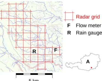
Scope of this analysis is the sub-catchment Wernersdorf. This small catchment (about 35 km2in area) is of particular interest, because as there are no more flow meters upstream, the possibilities for high water warnings for this place are limited. On the other hand the discharge measurements at Wernersdorf can be helpful to identify severe situations that may lead to hazards downstream. Our data shows that when-ever the flow meter at Wernersdorf had high peaks also the flow meters downstream had maxima after a significant time lag. Figure 1 presents a map of the Wernersdorf catchment, showing the radar grid and the location of rain gauge and flow meter.
In summer this region is often affected by rain showers. Short convective storms are the dominant flood producing processes in this area (Bl¨oschl et al., 2001). Sometimes the spatial extension of these showers is so small that a detec-tion is only possible by weather radar, while none of the rain gauges in that area reports precipitation.
The catchment response of this part of Austria can be con-sidered as flashy. The annual maximum daily precipitation occurs in late summer (Bl¨oschl et al., 2001). This is the pe-riod where the maximum annual flood peaks are measured.
630 R. Teschl and W. L. Randeu: A neural network model for short term river flow prediction
2
areal precipitation and in succession for the runoff volume than a single raingauge was able
to. The model presented here combines rain gauge, radar and runoff data.
1.1
Study Area
The study area is the Sulm catchment in the south-west of Styria, Austria. The whole basin
includes an area of 1105.7 square kilometres. Elevations reach from 263 m (above Mean Sea
Level, MSL) at the watershed outlet (Leibnitz) to 2125 m (MSL) on the Koralpe mountain
range. The average watershed slope is 11.9 %.
Scope of this analysis is the sub-catchment Wernersdorf. This small catchment (about 35 km²
in area) is of particular interest, because as there are no more flow meters upstream, the
possibilities for high water warnings for this place are limited. On the other hand the
discharge measurements at Wernersdorf can be helpful to identify severe situations that may
lead to hazards downstream. Our data shows that whenever the flow meter at Wernersdorf had
high peaks also the flow meters downstream had maxima after a significant time lag. Figure 1
presents a map of the Wernersdorf catchment, showing the radar grid and the location of rain
gauge and flow meter.
R
F
Radar grid
F
R
5 kmFlow meter
Rain gauge
A
Figure 1. Map of the Wernersdorf catchment
In summer this region is often affected by rain showers. Short convective storms are the
dominant flood producing processes in this area (Blöschl et al., 2001). Sometimes the spatial
extension of these showers is so small that a detection is only possible by weather radar, while
none of the rain gauges in that area reports precipitation.
Fig. 1. Map of the Wernersdorf catchment.
1.2 Available data
For the processing of the neural network model rain-gauge, flow meter and radar data were available. The datasets ex-tend over a 1-year period from January to December 2000. The temporal resolution of all datasets was assimilated to the temporal resolution of the runoff data which is 15 min. 1.2.1 Rain gauge and flow meter data
Because of the specific geographic and climatic situation the rain gauge and flow meter density is quite high compared to other parts of Austria. The outflow [m3/s] is known for all tributaries in the Sulm basin at 13 different sites. The time in-terval between the outflow-measurements is 15 min. Precipi-tation data are available from a network of rain gauges. The rain gauges are working on the tipping bucket principle with a resolution of 0.1 mm. The temporal resolution is 15 min. Data from 10 rain gauges are available. One rain gauge is lo-cated within the focused Wernersdorf sub-catchment. Both, rain gauge and flow meter data are officially controlled and verified by the Hydrographische Landesabteilung Steiermark (Department for Hydrography of the Province of Styria). 1.2.2 Radar data
To improve the spatial coverage, weather radar data from the Doppler weather radar station on Mt. Zirbitzkogel are used. The designated radar is a high-resolution C-band weather-radar. It has the following specifications:
– Altitude of the radar-station (m.s.l.): 2372 m – Time interval between measurements: 5 min
– 3-dB-Beamwidth: 1◦
– Minimum elevation angle: 0.8◦
– Spatial resolution of the volume element: 1 km3
(1×1×1 km3)
– Resolution in measured reflectivity: 14 levels of
rain-rate, converted from reflectivity Z by using a fixed rela-tionship (Z=200·R1.6)
– Instrumented range: 220 km
– Distance from the research area: to run from 42 km
(Ko-ralpe mountain range) to 80 km (Leibnitz, watershed outlet)
2 Neural network model
An Artificial Neural Network (ANN) is a method inspired by the human brain and nervous system. ANNs consist of a set of processing elements (neurons) operating in paral-lel. As the biological exemplar, the function of the ANN is determined basically by the connections between the neu-rons. ANNs have been used in various scientific fields to solve problems such as pattern recognition, particle identi-fication and classiidenti-fication. Furthermore ANNs are a proved and efficient method to model complex input-output relation-ships (Aliev, 2000). They learn the relationship directly from the data being modelled. Various fields of hydrology have been investigated with success with ANNs (Adeloye and De Munari, 2006). Particularly they have been used for rainfall-runoff modelling, river flow and flood forecasting e.g. Imrie et at. (2000); Kim and Barros (2001); Toth and Brath (2002). One of the most common neural network model is the Multi-Layer Perceptron (MLP), and this is the type of ANN used here. A MLP is a network that consists of three types of layers: input, hidden, and output layers. Patterns are in-troduced to the network via the input layer. In the hidden layers (one or more) the processing is done, the result for the given input pattern is produced and transmitted to the output layer. A MLP is a feed forward neural network. It is called “feed-forward” because all of the data information flows in one direction. The neurons of one layer are connected with the neurons of the following layer, there is no feedback. Here a fully connected MLP with one hidden layer is used.
The network function of an MLP is determined largely by the number of neurons in the different layers and the weighted connections between them. The product between the input p and the scalar weight w is calculated. Together with the scalar bias b, the argument of the transfer function
f is formed which produces the scalar output a.
a = f (wp + b) (1)
A number of transfer or activation functions exist. Fre-quently used however are non-linear sigmoid functions. Mul-tiple layers of neurons with nonlinear transfer functions like
R. Teschl and W. L. Randeu: A neural network model for short term river flow prediction 631 the sigmoid transfer function allow the network to learn
non-linear and non-linear relationships between input and output (De-muth and Beale, 1998). This is important for our application because the relationship between rainfall within a catchment and runoff at its outlet is known to be highly non-linear and complex (e.g. Hsu et al., 1995).
The logistic sigmoid transfer function takes the input, which may have any value between plus and minus infinity, and map the output to the range 0 to 1. Therefore the data must be scaled so that they always fall within the specified range. The disadvantages of sigmoid activation functions in the output layer, concerning the model’s ability to generalise beyond the calibration range, are given by Imrie et al. (2000). Solomatine and Dulal (2003) suggest to use an unbounded linear function in the output layer because it is able, to a cer-tain extent, to extrapolate beyond the range of the training data. Therefore the network used here incorporates a linear function in the output layer and logistic sigmoid activation functions in the input and hidden layers.
3 Preprocessing
In order to make the training process of the ANN more ef-fective the available data has been pre-processed. The goal of this process was to configure the ANN properly, more pre-cisely, to define an input vector and a network structure that best represent the watershed behaviour.
For this purpose the dataset has been investigated with sta-tistical methods in order to determine the correlation between input and output data. The cross-correlation is a measure of similarity of two signals. It is a function of the relative time between the signals. The cross correlation coefficient between rainfall and runoff, which was calculated by nor-malising the cross-correlation of the two signals, has been used to identify the time lag (offset) where the similarity is highest.
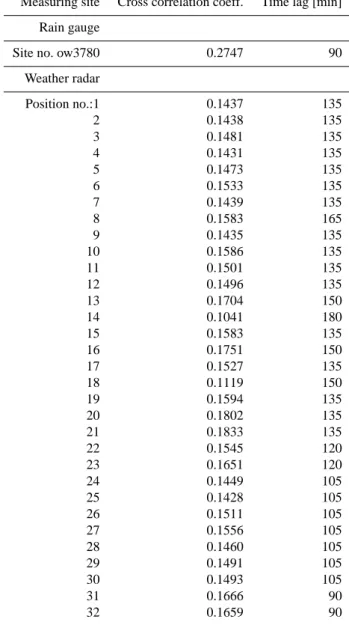
Rain gauge as well as weather radar series were investi-gated and the analysis showed that the time lags with the highest cross correlation coefficients between rainfall and runoff series lie between 90 to 180 min, depending on the po-sition within the catchment where the rainfall was measured. Table 1 shows the time lags in detail.
The analysis revealed that the correlation coefficients of rain gauge and radar measurements vary significantly. None of the radar data series obtained the maximum value of the rain gauge (0.2747). The poor correlation coefficients of the radar measurements can be explained by the fact that the radar does not detect low-level precipitation below 3 km (m.s.l.). High reaching convective rain cells however, the dominant source of high water and floods in this area, can be detected with good visibility by the weather radar station on Mt. Zirbitzkogel.
In order to answer the question whether the time lags of the radar pixels are though comprehensible for the
catch-Table 1. Time lag with the maximum cross correlation coefficient
between rainfall and runoff series. (The position number refers to the position of the 1 km×1 km radar pixels within the catchment top down line by line.)
Measuring site Cross correlation coeff. Time lag [min] Rain gauge
Site no. ow3780 0.2747 90 Weather radar Position no.:1 0.1437 135 2 0.1438 135 3 0.1481 135 4 0.1431 135 5 0.1473 135 6 0.1533 135 7 0.1439 135 8 0.1583 165 9 0.1435 135 10 0.1586 135 11 0.1501 135 12 0.1496 135 13 0.1704 150 14 0.1041 180 15 0.1583 135 16 0.1751 150 17 0.1527 135 18 0.1119 150 19 0.1594 135 20 0.1802 135 21 0.1833 135 22 0.1545 120 23 0.1651 120 24 0.1449 105 25 0.1428 105 26 0.1511 105 27 0.1556 105 28 0.1460 105 29 0.1491 105 30 0.1493 105 31 0.1666 90 32 0.1659 90
ment, despite the low correlation coefficients, the radar pixel directly above the rain gauge was examined and compared with the time lag of the rain gauge.
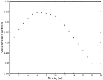
The cross correlation between gauge measured rainfall and runoff becomes a maximum at a shift of 90 min (see Fig. 2). The radar measurement in about 3 km altitude above the rain gauge site (no. 24) exhibits a shift of 105 min (see Fig. 3). The difference – 15 min prior to the rain gauge – is connected with the temporal resolution of the time series (it is the short-est time lag which can be identified) and can be explained by the different altitude of radar and rain gauge measurements:
632 R. Teschl and W. L. Randeu: A neural network model for short term river flow prediction
7 In order to answer the question whether the time lags of the radar pixels are though comprehensible for the catchment, despite the low correlation coefficients, the radar pixel directly above the rain gauge was examined and compared with the time lag of the rain gauge.
The cross correlation between gauge measured rainfall and runoff becomes a maximum at a shift of 90 minutes (see Figure 2). The radar measurement in about 3 km altitude above the rain gauge site (no. 24) exhibits a shift of 105 minutes (see Figure 3). The difference - 15 minutes prior to the rain gauge – is connected with the temporal resolution of the time series (it is the shortest time lag which can be identified) and can be explained by the different altitude of radar and rain gauge measurements: aloft and on the ground. Therefore the values of the radar seem comprehensible.
0 2 4 6 8 10 12 14 16 18 20 0.245 0.25 0.255 0.26 0.265 0.27 0.275 0.28 Time lag [h/4] C ro s s c o rr e la ti o n c o e ff ic ie n t
Figure 2. Cross correlation analysis between rain-gauge and runoff measurements Fig. 2. Cross correlation analysis between rain-gauge and runoff
measurements. 8 0 2 4 6 8 10 12 14 16 18 20 0.132 0.134 0.136 0.138 0.14 0.142 0.144 0.146 0.148 Time lag [h/4] C ro s s c o rr e la ti o n c o e ff ic ie n t
Figure 3. Cross correlation analysis between radar (radar pixel no. 24, directly above raingauge) and runoff measurements.
The correlation analysis suggests that a forecast for 6 time lags (90 minutes) is appropriate. This is the shortest shift between precipitation and runoff series that could be found.
The correlation analysis also suggests that it makes sense to define an input vector with 6 to 12 antecedent rainfall measurements depending on the time lag where the maximum correlation between runoff and rainfall was measured. But this would lead to a huge number of input parameters and an effective training would not be possible. Therefore the dimension of the input vector had to be reduced. A method to do this is for example the principal component analysis (e.g. Demuth and Beale, 1998) which eliminates those components contributing the least to the variation in the data set. But this means that only a few radar measurements would be part of the input vector and the main advantage of the radar the gap less spatial coverage would be lost. The detection of small convective shower cells would not be ensured.
The method used to solve this conflict was to group radar measurements with the same time lag, leading to a smaller input vector. The radar pixels showing the same time lag to the runoff on average were summed up. This leads to groups of several pixels herein after referred to as
Fig. 3. Cross correlation analysis between radar (radar pixel no. 24,
directly above raingauge) and runoff measurements.
aloft and on the ground. Therefore the values of the radar seem comprehensible.
The correlation analysis suggests that a forecast for 6 time lags (90 min) is appropriate. This is the shortest shift between precipitation and runoff series that could be found.
The correlation analysis also suggests that it makes sense to define an input vector with 6 to 12 antecedent rainfall mea-surements depending on the time lag where the maximum correlation between runoff and rainfall was measured. But this would lead to a huge number of input parameters and an effective training would not be possible. Therefore the dimension of the input vector had to be reduced. A method to do this is for example the principal component analysis (e.g. Demuth and Beale, 1998) which eliminates those com-ponents contributing the least to the variation in the data set.
Table 2. Time lag with the maximum cross correlation coefficient
between clusters and runoff series.
Measuring site Cross correlation coeff. Time lag [min] Rain gauge
Site no. ow3780 0.2747 90 Cluster no.:1 0.1705 90 2 0.1650 105 3 0.1729 120 4 0.1907 135 5 0.1623 150 6 0.1583 165 7 0.1041 180
But this means that only a few radar measurements would be part of the input vector and the main advantage of the radar the gap less spatial coverage would be lost. The detection of small convective shower cells would not be ensured.
The method used to solve this conflict was to group radar measurements with the same time lag, leading to a smaller input vector. The radar pixels showing the same time lag to the runoff on average were summed up. This leads to groups of several pixels herein after referred to as clusters represent-ing the amount of precipitation in this area. Table 2 shows correlation coefficient and time lag of the precipitation mea-surements forming the input vector. The rain gauge measure-ments are left unmodified. They are not grouped with radar measurements showing the same 90 min time lag. Cluster 1 to 7 represent summations of radar time series showing the same time lag with respect to the runoff data. The correlation coefficients of the clusters are often higher than those of the radar pixels forming the cluster. The advantage of this tech-nique is that information of each pixel above the catchment is still represented in the dataset. Because of the bigger clusters the information where exact a small convective shower cell occurred is lost but the rainfall amount within the area repre-sented by the cluster is available and the time lag when the rainfall shows the highest correlation with the runoff series is known.
Besides rainfall measurements, it may also be useful to present antecedent runoff measurements to the ANN. Sud-heer et al. (2002) propose the partial autocorrelation to de-cide how much former runoff values should be included into the input vector, see Fig. 4. The time lag before the correla-tion falls in the 95% confidence band is used as an indicator. According to this algorithm the input vector should contain runoff values from up to 8 antecedent intervals. In our case, where a forecast for 90 min is made, 5 antecedent runoff mea-surements are not available. Therefore networks with up to 3 antecedent runoff measurements were tested.
R. Teschl and W. L. Randeu: A neural network model for short term river flow prediction 633 10 1 2 3 4 5 6 7 8 9 10 -1 -0.8 -0.6 -0.4 -0.2 0 0.2 0.4 0.6 0.8 Time lags [h/4] P a rt ia l a u to c o rr e la ti o n
Partial autocorrelation coefficient 95 % Confidence band
Figure 4. Partial auto correlation analysis of the runoff data.
ANN Architecture
For identifying the architecture of an ANN associated with determining the number of neurons in each layer, the trial-and-error approach is still the most common (Imrie et at.,2000; Pan and Wang, 2004; Toth et al. 2000). Some software packages perform the trial-and-error optimisation automatically. The architecture anyway is highly dependent on the problem to be solved and so no general solution can be given.
An area of conflict is that a small network may have insufficient degrees of freedom (weights and biases) to represent the relationship between rainfall and runoff, and a large network with many weights to be adapted may memorise fluctuations in the training data and is therefore not able to generalise.
10 1 2 3 4 5 6 7 8 9 10 -1 -0.8 -0.6 -0.4 -0.2 0 0.2 0.4 0.6 0.8 Time lags [h/4] P a rt ia l a u to c o rr e la ti o n
Partial autocorrelation coefficient 95 % Confidence band
Figure 4. Partial auto correlation analysis of the runoff data.
ANN Architecture
For identifying the architecture of an ANN associated with determining the number of neurons in each layer, the trial-and-error approach is still the most common (Imrie et at.,2000; Pan and Wang, 2004; Toth et al. 2000). Some software packages perform the trial-and-error optimisation automatically. The architecture anyway is highly dependent on the problem to be solved and so no general solution can be given.
An area of conflict is that a small network may have insufficient degrees of freedom (weights and biases) to represent the relationship between rainfall and runoff, and a large network with many weights to be adapted may memorise fluctuations in the training data and is therefore not able to generalise.
Fig. 4. Partial auto correlation analysis of the runoff data.
ANN architecture
For identifying the architecture of an ANN associated with determining the number of neurons in each layer, the trial-and-error approach is still the most common (Imrie et al., 2000; Pan and Wang, 2004; Toth et al., 2000). Some software packages perform the trial-and-error optimisation automatically. The architecture anyway is highly dependent on the problem to be solved and so no general solution can be given.
An area of conflict is that a small network may have insuf-ficient degrees of freedom (weights and biases) to represent the relationship between rainfall and runoff, and a large net-work with many weights to be adapted may memorise fluc-tuations in the training data and is therefore not able to gen-eralise.
Therefore the method used to determine the architecture of the ANN was to start with a small network (one hidden layer and three hidden nodes), to increase the number of nodes and to choose the network with the best performance. During the training process the error on the validation set (mean square error) was monitored. When the validation error increased the training was stopped and the minimum of the validation error was taken as indicator for the performance. Thus a net-work with twelve nodes in one hidden layer was determined. Essential for a good performance of an MLP is cautious selection of the training validation and test data sets. In the present case where data of a period of one year are available the selection of the subsets for the training validation and test process is even more eminent. Eventually a method was used that ensures that each of the tree subsets contains ran-dom data from all seasons. Therefore the whole data set was
12 0 2400 4400 8400 10400 12400 14000 0 0.5 1 1.5 2 2.5 3 3.5 4 4.5 Time [h/4] R u n o ff [ m ³/ s ] Predicted runoff Measured runoff
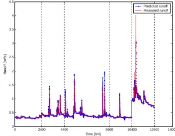
Figure 5: Comparison between predicted and measured runoff series of the test dataset.
The parameters RMSE: 0.0596 and R² 0.9489 suggest a very good performance. In general, a
R² value greater than 0.9 indicates a very satisfactory model performance, while a R² value in
the range 0.8 – 0.9 signifies a good performance and values less than 0.8 indicate an unsatisfactory model performance (Coulibaly and Baldwin,2005).
The R² value has to be treated with caution, because it contains the mean of the observed runoff values. Because of high runoff values of the last subset of the training dataset the mean value over the whole training set is 0.4884. Table 3 gives the RMSE and R² values for the five subsets of the training data.
Fig. 5. Comparison between predicted and measured runoff series
of the test dataset.
Table 3. RMSE and R2of the training set and the five subsets separately. The number of the subset refers to the occurrence in Fig. 5. RMSE R2 Subset 1 0.0084 0.8863 2 0.0396 0.8685 3 0.0554 0.8566 4 0.0365 0.7419 5 0.1136 0.8306 Overall 0.0596 0.9489
divided into rainfall events and their corresponding runoff hydrographs. These events where classified into the seasons they belong to and training validation and test subset where formed by randomly assigning events from all seasons to all subsets.
4 Results and discussion
The simulation performance of the ANN model was evalu-ated on the basis of Root Mean Square Error (RMSE) and
R2efficiency coefficient by Nash and Sutcliffe (1970). In Fig. 5 the comparison between predicted and measured runoff series can be seen. The output of the model, simu-lated with test data, shows a good agreement with the target concerning prediction of the time of maximum concentra-tion. As mentioned above training validation and test data contain subsets from all seasons. In Fig. 5 the vertical grid lines separate the different subsets.
634 R. Teschl and W. L. Randeu: A neural network model for short term river flow prediction
13 Table 3: RMSE and R² of the training set and the five subsets separately. (The number of the subset refers to the occurrence in Fig.5.
RMSE R² Subset 1 0.0084 0.8863 2 0.0396 0.8685 3 0.0554 0.8566 4 0.0365 0.7419 5 0.1136 0.8306 Overall 0.0596 0.9489
Table 3 shows that the performance of all subsets except subset 4 can be considered as good. The high RMSE of subset 5 is due to the underestimation of the highest peak. Figure 6 shows this subset in detail.
0 200 400 600 800 1000 1200 1400 1600 1800 2000 0.5 1 1.5 2 2.5 3 3.5 4 4.5 R u n o ff [ m ³/ s ] Time [h/4] Predicted runoff Measured runoff
Figure 6: Comparison between predicted and measured runoff series of the subset 5 of the testset.
Figure 6 shows that the dynamics in the hydrograph are captured quite well by the model, while the highest peak is underestimated. The underestimation is believed to result from the
Fig. 6. Comparison between predicted and measured runoff series
of the subset 5 of the testset.
Table 4. RMSE and R2of the validation set and the four subsets separately. The number of the subset refers to the occurrence in Fig. 7. RMSE R2 Subset 1 0.0083 0.9497 2 0.0919 0.7185 3 0.0322 0.892 4 0.1071 0.8694 Overall 0.0645 0.9412
The parameters RMSE: 0.0596 and R2: 0.9489 suggest a very good performance. In general, a R2value greater than 0.9 indicates a very satisfactory model performance, while a
R2value in the range 0.8–0.9 signifies a good performance and values less than 0.8 indicate an unsatisfactory model per-formance (Coulibaly and Baldwin, 2005).
The R2 value has to be treated with caution, because it contains the mean of the observed runoff values. Because of high runoff values of the last subset of the training dataset the mean value over the whole training set is 0.4884. Table 3 gives the RMSE and R2 values for the five subsets of the training data.
Table 3 shows that the performance of all subsets except subset 4 can be considered as good. The high RMSE of sub-set 5 is due to the underestimation of the highest peak. Fig-ure 6 shows this subset in detail.
Figure 6 shows that the dynamics in the hydrograph are captured quite well by the model, while the highest peak is underestimated. The underestimation is believed to result from the fact that the training dataset did not contain such
14 fact that the training dataset did not contain such high discharge values. This assumption is supported by an analysis of the vaildation dataset.
0 3000 5000 8500 10500 0 0.5 1 1.5 2 2.5 3 3.5 4 Time [h/4] R u n o ff [ m ³/ s ] Predicted runoff Measured runoff
Figure 7: Comparison between predicted and measured runoff series of the validation dataset.
Again the highest peak is underestimated. Obviously the effect the unbounded linear function in the output layer has, to help the ANN extrapolate beyond the range of the training data is not significant. Figure 8 shows the affected subset 4 in detail.
Fig. 7. Comparison between predicted and measured runoff series
of the validation dataset.
15 0 200 400 600 800 1000 1200 1400 1600 1800 2000 0.5 1 1.5 2 2.5 3 3.5 4 R u n o ff [ m ³/ s ] Time [h/4] Predicted runoff Measured runoff
Figure 8: Comparison between predicted and measured runoff series of the subset 4 of the validation set.
Concerning RMSE and R² the performance of the test and validation set is more or less equal. The validation subset shown in Fig. 8 also has with 0.1071 a high RMSE value. Table 4 shows the details.
Table 4: RMSE and R² of the validation set and the four subsets separately. (The number of the subset refers to the occurrence in Fig.7.
RMSE R² Subset 1 0.0083 0.9497 2 0.0919 0.7185 3 0.0322 0.892 4 0.1071 0.8694 Overall 0.0645 0.9412
Fig. 8. Comparison between predicted and measured runoff series
of the subset 4 of the validation set.
high discharge values. This assumption is supported by an analysis of the vaildation dataset.
Again the highest peak is underestimated. Obviously the effect the unbounded linear function in the output layer has, to help the ANN extrapolate beyond the range of the training data, is not significant. Figure 8 shows the affected subset 4 in detail.
Concerning RMSE and R2the performance of the test and validation set is more or less equal. The validation subset shown in Fig. 8 also has with 0.1071 a high RMSE value. Table 4 shows the details.
Acknowledgements. The authors would like to thank W. Verw¨uster
form the Hydrographische Landesabteilung for providing the flow meter and rain gauge data and the anonymous reviewers for
R. Teschl and W. L. Randeu: A neural network model for short term river flow prediction 635
their helpful suggestions and valuable comments on the original manuscript.
Edited by: P. P. Alberoni Reviewed by: two referees
References
Adeloye, A. J. and De Munari, A.: Artificial neural network based generalized storage–yield–reliability models using the Levenberg-Marquardt algorithm, J. Hydrol., 326(1–4), 215–230, 2006.
Aliev, R., Bonfig, K. W., and Aliew, F.: Soft Computing: Eine grundlegende Einf¨uhrung, Verlag Technik, Berlin, 2000. Bl¨oschl, G., Merz, R., and Piock-Ellena, U.: Flash-Flood Risk
As-sessment under the Impacts of Land Use Changes and River En-gineering Works, Final Report, Institute of Hydraulics, Hydrol. Water Resour. Manage., Vienna University of Technology, 2001. Coulibaly, P. and Baldwin, C. K.: Nonstationary hydrological time series forecasting using nonlinear dynamic methods, J. Hydrol., 307, 164–174, 2005.
Demuth, H. and Beale, M.: MATLAB Neural Networks Toolbox – User’s Guide, Fifth Printing – Version 3, 1998.
Hsu, K., Vijai Gupta, H., and Sorooshian, S.: Artificial neural net-work modeling of the rainfall-runoff process, Water Resour. Res., 31(10), 2517–2530, 1995.
Imrie, C. E., Durucan, S., and Korre, A.: River flow prediction using artificial neural networks: generalisation beyond the calibration range, J. Hydrol., 233, 138–153, 2000.
Kim, G. and Barros, A. P.: Quantitative flood forecasting using mul-tisensor data and neural networks, J. Hydrol., 246, 45–62, 2001. Nash, J. E. and Sutcliffe, J. V.: River flow forecasting through con-ceptual models I: A discussion of principles, J. Hydrol., 10, 282– 290, 1970.
Pan, T.-Y. and Wang, R.-Y.: State space neural networks for short term rainfall-runoff forecasting, J. Hydrol., 297, 34–50, 2004. Solomatine, D. P. and Dulal, K. N.: Model trees as an alternative to
neural networks in rainfall–runoff modelling, Hydrological Sci-ences – Journal des SciSci-ences Hydrologiques, 48, 399–411, 2003. Sudheer, K. P., Gosain, A. K., and Ramasastri, K. S.: A data driven algorithm for constructing ANN based rainfall-runoff models, Hydrol. Processes, 16, 1325–1330, 2002.
Smith, P. L. (Chairman), Atlas, D., Bluestein, H. B., Chandrasekar, N. V., et al.: Weather Radar Technology Beyond NEXRAD, Committee on Weather Radar Technology Beyond NEXRAD, National Research Council, ISBN: 0-309-08466-0, 96 pages, 2002.
Teschl, R. and Randeu, W. L.: An Artificial Neural Network-based Rainfall-Runoff Model using gridded Radar Data. Third European Conference on Radar in Meteorology and Hydrology (ERAD), Visby, Island of Gotland, Sweden, Paper nr.: ERAD3-A-00163, 2004.
Toth, E., Brath, A., and Montanari, A.: Comparison of short-term rainfall prediction models for real-time flood forecasting, J. Hy-drol., 239, 132–147, 2000.