HAL Id: insu-02957353
https://hal-insu.archives-ouvertes.fr/insu-02957353
Submitted on 24 Nov 2020
HAL is a multi-disciplinary open access
archive for the deposit and dissemination of
sci-entific research documents, whether they are
pub-lished or not. The documents may come from
teaching and research institutions in France or
abroad, or from public or private research centers.
L’archive ouverte pluridisciplinaire HAL, est
destinée au dépôt et à la diffusion de documents
scientifiques de niveau recherche, publiés ou non,
émanant des établissements d’enseignement et de
recherche français ou étrangers, des laboratoires
publics ou privés.
Distributed under a Creative Commons Attribution| 4.0 International License
Hydromechanical insight of fracture opening and closure
during in-situ hydraulic fracturing in crystalline rock
Nathan Dutler, Benoît Valley, Valentin Gischig, Mohammadreza Jalali,
Bernard Brixel, Hannes Krietsch, Clément Roques, Florian Amann
To cite this version:
Nathan Dutler, Benoît Valley, Valentin Gischig, Mohammadreza Jalali, Bernard Brixel, et al..
Hy-dromechanical insight of fracture opening and closure during in-situ hydraulic fracturing in crystalline
rock. International Journal of Rock Mechanics and Mining Sciences, Pergamon and Elsevier, 2020,
135, pp.104450. �10.1016/j.ijrmms.2020.104450�. �insu-02957353�
International Journal of Rock Mechanics & Mining Sciences 135 (2020) 104450
Available online 24 September 2020
1365-1609/© 2020 The Authors. Published by Elsevier Ltd. This is an open access article under the CC BY license (http://creativecommons.org/licenses/by/4.0/).
Hydromechanical insight of fracture opening and closure during in-situ
hydraulic fracturing in crystalline rock
Nathan Dutler
a,*, Benoît Valley
a, Valentin Gischig
b, Mohammadreza Jalali
c, Bernard Brixel
d,
Hannes Krietsch
d, Cl´ement Roques
d,e, Florian Amann
caCenter for Hydrogeology and Geothermics, University of Neuchˆatel, Neuchˆatel, Switzerland bCSD Engineers, Bern, Switzerland
cDepartment of Engineering Geology and Hydrogeology, RWTH Aachen, Aachen, Germany dDepartment of Earth Science, ETH Zurich, Zurich, Switzerland
eUniversity Rennes 1, G´eosciences Rennes, UMR 6118, Av. du G´en´eral Leclerc, 35042, Rennes, France
A R T I C L E I N F O
Keywords:
Hydraulic fracturing Hydraulic jacking
Diagnostic fracture injection tests (DFIT)
Fluid-rock mass coupling Fractured rock Diagnostic plots
A B S T R A C T
Six hydraulic fracturing (HF) experiments were conducted in situ at the Grimsel Test Site (GTS), Switzerland, using two boreholes drilled in sparsely fractured crystalline rock. High spatial and temporal resolution moni-toring of fracture fluid pressure and strain improve our understanding of fracturing dynamics during and directly following high-pressure fluid injection. In three out of the six experiments, a shear-thinning fluid with an initial static viscosity approximately 30 times higher than water was used to understand the importance of fracture leak-off better. Diagnostic analyses of the shut-in phases were used to determine the minimum principal stress magnitude for the fracture closure cycles, yielding an estimate of the effective instantaneous shut-in pressure (effective ISIP) 4.49±0.22 MPa. The jacking pressure of the hydraulic fracture was measured during the pressure- controlled step-test. A new method was developed using the uniaxial Fibre-Bragg Grating strain signals to es-timate the jacking pressure, which agrees with the traditional flow versus pressure method. The technique has the advantage of observing the behavior of natural fractures next to the injection interval. The experiments can be divided into two groups depending on the injection location (i.e., South or North to a brittle-ductile S3 shear zone). The experiments executed South of this zone have a jacking pressure above the effective ISIP. The proximity to the S3 shear zone and the complex geological structure led to near-wellbore tortuosity and het-erogeneous stress effects masking the jacking pressure. In comparison, the experiments North of the S3 shear zone has a jacking pressure below the effective ISIP. This is an effect related to shear dislocation and fracture opening. Both processes can occur almost synchronously and provide new insights into the complicated mixed- mode deformation processes triggered by high-pressure injection.
1. Introduction
The dynamic injection pressure response monitored during hydraulic fracturing treatments in fractured reservoirs contains information on reservoir hydraulic and geomechanical properties which are, in turn, critical to describe and predict hydromechanical processes. However, the interpretation of pressure data is generally not trivial as it is affected by structures at different scales ranging from a single fracture to com-plex interactions within a three-dimensional fracture network. Histori-cally, the transient pressure analyses (TPA) that are used as a diagnostic tool relied entirely on analytical models of fluid flow, without
hydromechanical coupling. The first and most straightforward solution to constant fluid injection/withdrawal, which governs radial flow in a porous medium, was introduced by Theis1 for groundwater flow. Orig-inal work for TPA was mainly driven by the oil & gas industry, consid-ering both Newtonian and non-Newtonian fluids (e.g., Ref. 2). Subsequently, the TPA was also extended to geothermal wells, including the two-phase flow of water and steam, adsorption of steam and pres-surized reservoirs (more in Zarrouk & McLean3). The ’dual-porosity’
model of Warren & Root4 was the earliest attempt to represent fractured
reservoirs. Later, Barker5 introduced the generalized radial flow model
for fractured reservoirs, which was extended to fractal fracture networks.6,7
* Corresponding author.
E-mail address: [email protected] (N. Dutler).
Contents lists available at ScienceDirect
International Journal of Rock Mechanics and Mining Sciences
journal homepage: http://www.elsevier.com/locate/ijrmmshttps://doi.org/10.1016/j.ijrmms.2020.104450
International Journal of Rock Mechanics and Mining Sciences 135 (2020) 104450
2
1.1. Background on transient pressure analysis (TPA)
Various diagnostic pressure representations, such as log-log plots, semi-log plots, and various time manipulation techniques, have been developed to interpret the evolution of fluid pressure with time during high-pressure fluid injection (see Ref. 8; for a review). Many methods
have the aim to identify diagnostic pressure levels and derive stress estimates (see Ref. 9; for a review). In tight formations, diagnostic fracture
injection tests (DFIT) are used to estimate key parameters, such as the
minimum principal stress, fluid leak-off (fluid loss from the hydraulic fracture towards the rock matrix or other natural fractures), perme-ability, and pore pressure. Once injection stops, i.e. the injection interval is shut-in, the pressure rapidly drops at first, followed by a regime with a slower pressure decay at late times. The point of transition between the two regimes measured immediately after shut-in is referred to as the
instantaneous shut-in pressure (ISIP) and is often considered to be a
reasonable approximation of the minimum in-situ principal stress magnitude for fracture fluids with low viscosity in moderately fractured crystalline rock mass. Authors working in the oil & gas industry argue that the fracture closure pressure may be a better estimate for tight rock formations. Problems generally arise due to the indifferent use of ISIP and fractures closure pressure in the literature.9
The analysis of DFIT based on G-function and its derivative intro-duced by Nolte10 also allows to quantify the minimum principal stress magnitude, under the assumptions that (1) leak-off is not pressure-dependent and (2) fracture compliance is assumed to be con-stant during fracture closure. Barree et al.11 introduced a method of analysis using the G-function and its derivative drawing a line from the origin to the tangent of the G*dp/dG. The method is referred to as the ‘Barre tangent method’ following the terminology after Jung et al.12 It was challenged by McClure et al.13 and McClure et al.,14 who pointed
out that this method has no theoretical justification. McClure et al.13,14
and Jung et al.12 proposed the ‘compliance method’ to estimate the
fracture closure, but it tends to reflect only the onset of fracture closure. Wang & Sharma15 pointed out that the upward curved G*dp/dG is
caused by the fracture-pressure dependent leak-off with compliance variation during fracture closure. Therefore, they proposed to pick the closure, in between the compliance and Barre tangent method, which is known as the ‘variable compliance method’ and should give a better estimate of the minimum principal stress component. McClure et al.16
defined ‘contact pressure’, which is equivalent to the definition of ‘closure pressure’.14 It is defined as the pressure, where the contact of
the fracture walls causes a measurable change in the system stiffness caused by the contact of fracture walls.
The method uses the G-function and the minimum of dp/dG needs to be identified prior to contact pressure. If the hydraulic fracture intersects highly conductive natural, pre-existing fractures, the dp/dG curve decrease monotonically and challenges this method. Under these con-ditions the immediate fracture closes and can be estimated using the effective ISIP. The point of the weak minimum of the dp/dG curve needs to be identified. Then, the G time of this minimum is used and a tangent is set to the point on the pressure curve to extrapolate the pressure versus G-time back to zero, which is the effective ISIP.
1.2. Hydromechanics
Field experiments conducted on single fractures have brought detailed insights on the hydromechanical properties of single fractures and their behavior during fluid injection.17 Such behavior can be
described by an empirical closure law including hyperbolic,18,19
semi--logarithmic20,21 or statistical distribution22 combining normal stress and
normal closure using laboratory experiments (e.g., step-pressure tests or purely mechanical tests). A hysteresis effect is typically observed in the uniaxial strain component measured across the fracture when comparing the aperture state before and after the opening and closing cycle. This effect, however, cannot be detected from a diagram of in-jection flow-rate versus inin-jection pressure.23
Fracture roughness induces a high spatial variability in local me-chanical apertures. Zones, where the two fracture surfaces are in contact (contact area), may be strongly dependent on the scaling of the fracture roughness and the normal stress acting on the fracture plane. Changes in contact area lead to non-linear empirical closure relationships (assuming constant mechanical parameters) and spatial distribution of local mechanical apertures may create strong flow channelization and tortuosity, which in turn impacts fracture transmissivity.24 Laboratory
experiments on single fractures are typically performed at the centi-meter or centi-meter-scale (0.01–1 m). It is well known that mechanical and hydraulic apertures are generally not equivalent.25–27 In-situ field
ex-periments investigate processes that involve fracture networks. Me-chanical apertures are therefore challenging to determine in situ. Based
Nomenclature
C Diffusion coefficient [m2/s]
cL Carter leak-off coefficient [m/s0.5]
Ct Total system storage coefficient [m3/MPa]
G G-function [dimensionless]
g g-function [dimensionless]
K Consistency parameter of fluid [Pa*s, cPs]
n Flow behavior parameter [dimensionless]
p, pinj,pexp Fluid pressure [MPa] pformation Formation pressure [MPa]
q, qinj Volumetric flow rate [l/min]
qave Averaged volumetric flow rate [l/min]
t Time [s]
tshut− in Time of shut-in [s]
tend Time of the test end [s]
ta,t The actual shut-in time [s] V Fluid volume [m3]
vL Carter leak-off velocity [m/s]
γ’ Shear rate [Hz] p Pressure recovery [MPa]
p’ Bourdet derivative of pressure recovery [MPa]
δexp FBG reading [μm]
σi for i = 1,2,3, principal stress magnitudes [MPa]
σn Normal stress [MPa]
τ Shear stress [MPa]
μf Effective viscosity [Pa*s, cPs]
Abbreviations
ATV Acoustic borehole televiewer DFIT Diagnostic fracture injection tests FBG Fibre-bragg grating
HF Hydraulic fracturing HS Hydraulic shearing
ISC In-situ stimulation and circulation ISIP Instantaneous shut-in pressure JP Jacking pressure
OPTV Optical borehole televiewer TPA Transient pressure analysis
F Frac cycle
RF Refrac cycle
SR Pressure-controlled step-test XSW Xanthan-salt-water
on hydraulic tests, one can only assess fracture transmissivity as a proxy for hydraulic aperture, which encompasses the effects of fracture roughness on the resistance to flow.
1.3. Research objectives
This study extends the analysis of presented results from in-situ hy-draulic fracturing experiments performed at the Grimsel Test Site (GTS) in Switzerland,28 which were executed in the framework of the In-situ
Stimulation and Circulation (ISC) project.29 The unique and high level of
experimental control allows us to extend the knowledge of the stress state. DFIT methods paired with fracture opening pressure are used to constrain the minimum principal stress magnitude. In addition, the hydraulic fracture intersecting the open wellbore section from geophysical logging and seismic cloud observation constrain the orien-tation of the minimum principal stress and allow to derive a stress tensor for the HF experiments.
2. Rock mass characterization and experimental setup
2.1. Rock mass characterization
The rock volume investigated is located in the southern part of the GTS and is accessed by an array of boreholes monitoring deformation (i. e., referred to FBS1, -2, -3), fluid pressure (not used in this study, PRP1, -2, -3) and seismicity (GEO-1 to − 4, not shown) (Fig. 1a). Additionally, two 146-mm diameter boreholes (INJ1, -2) were drilled to high-pressure fluid injection. During the HF experiments, one of the boreholes was used for the injection while the other borehole was used as an additional pressure monitoring borehole.
The host rock consists of the Grimsel Granodiorite. It has a magmatic fabric characterized by a strong textural overprinting that occurred during Alpine orogeny resulting in a pervasive foliation oriented 157/ 75◦. The following properties were measured in the laboratory under drained conditions: Youngs-modulus, 20–40 GPa,33 Poisson’s ration,
0.1–0.2,33 critical fracture toughness, 0.7–1.7 MPa√̅̅̅̅̅m34 and tensile strength, 5.6–14.7 MPa.34
The moderately fractured host rock is crosscut by two sets of shear zones that differ in terms of deformation history and orientation (Fig. 1a +b). The shear zones of the first set (referred to as S1.0, S1.1, S1.2, and S1.3) experienced retrograde brittle deformation. They have an ENE- WSW strike and dip towards SSE. The shear zones of the second set (referred to as S3.1 and S3.2) are associated with the reactivation of two pre-Alpine, E-W-striking metabasic dikes. A densely fractured zone (up to 20 fractures per meter, depending on location) was identified in the eastern part of the test volume in between the two S3 shear zones. An
increase in fracture density was also observed around the S1 shear zone. Two fracture sets are associated with the S3 zone, where set K1 is ori-ented similar to the S3 zone, and set K2 strikes NNW-SSE and dips to-wards ENE (Fig. 1c).30,32,35 A fracture is considered here as a
visually-detectable structure whose trace could be observed on an op-tical (OPTV) or acoustic (ATV) borehole log. We do not account for grain-scale micro-cracks in this study.
The ambient in-situ pore pressure based on the cross-hole hydraulic testing setup deployed prior to the HF experiments in March 2017 (field setup not shown here) is presented as a function of true vertical depth (tvd) in Fig. 1d. With increasing depth, the pore pressure increases, whereas the tunnel level is a natural drainage level. The pore pressure is around 250 kPa and 500 kPa for experiments on S3 and S1 structures (Fig. 1d). Note that on the time scales investigated in this study, pressure diffusion (hence flow) is primarily controlled by fractures. This is a consequence of the very low hydraulic transmissivity of the host rock (10−14 - 10−13 m2/s, Jalali et al.36).
The stress field was measured on the southern side of the AU cavern in unfractured rock at distances greater than 20 m from brittle-ductile shear zones (referred as unperturbed stress tensor by Krietsch et al.31).
Additionally, the stress state was characterized up to a few meters to-wards the S3.1 shear zone. With decreasing distance to the shear zones, the stress field appears to rotate and decrease in magnitudes (i.e., especially the minimum principal stress). The stress state close to the shear zones is referred to as the perturbed stress state31 (Fig. 1a and
Table 1). The injection boreholes (INJ1, -2) were designed and drilled to align with the intermediate stress direction.
2.2. Experimental setup
In an earlier study,28 we showed that the location of the performed
experiments significantly influences the measured hydraulic and rock mass deformation response (see Fig. 1a for injection location). We can divide the experimental responses depending on the main geological structures, which will influence the response e.g., S1 (HF1, HF2, and HF6) and S3 (H3, HF5, and HF8) domain. We refer to Dutler et al.28 for a
tabular summary of the tests performed in this experiment. The injection interval measured 1.0 m and was equipped with a pressure transducer and flow lines. A data acquisition system recorded the pressure in the Fig. 1. a) Overview of the setup: the injection
loca-tion in the injecloca-tion boreholes (INJ1 and INJ2), the Fiber-Bragg Grating (FBG) sensors in the FBS bore-holes, tunnels, and shear-zones30 inclusive additional
new S1.0 interpolation). The lower stereonet in-dicates the stress field.31 b) The geological model is
presented in three different structural domains,32 and
c) the two lower stereonets presenting the fractures associates with the S1 (red) and S3 (green) faults.28 d)
The pressure head (pore pressure) is given for the true vertical depth (tvd) and is differentiated into two major structures before the HF experiment. (For interpretation of the references to color in this figure legend, the reader is referred to the Web version of this article.)
Table 1
Magnitudes of the unperturbed and perturbed stress state from Krietsch et al.31].
Stress state σ1[MPa] σ2[MPa] σ3[MPa] Unperturbed 14.4 10.2 8.6 Perturbed 13.1 8.2 6.5
International Journal of Rock Mechanics and Mining Sciences 135 (2020) 104450
4
injection interval of the INJ boreholes, the flow rate, and the packer pressure in the injection intervals with a sampling rate of 20 Hz. The injection pressure and flow were measured up-hole at the water injec-tion lines next to the injecinjec-tion pump. All acquisiinjec-tion systems were time-synchronized.
The rock mass deformation monitoring system consists of 60 Fibre- Bragg Grating (FBG) sensors in the three FBS boreholes (Fig. 1). 20 FBG sensors were installed along each FBS borehole to characterize the strain field in both intact and fractured rock. The FBG sensors have a base length of 1.0 m, and the sensors were pre-strained to enable monitoring of extension and compression. The cross-hole distances be-tween deformation monitoring intervals and the injection interval ranged between 3 m and 35 m. In this study, we consider positive strain as expansion. The strain data were recorded with a 1 kHz sampling rate. An extensive description of the ISC project, including the complete monitoring setup, characterization steps, and stimulation steps, can be found in Doetsch et al.37
2.3. Injection protocol
The flow rate qinj and the injection pressure pinj from test HF2 and HF8 are presented in Fig. 2a and b, respectively. HF2 is representative for tests close to S1 shear zones and HF8 is characteristic for tests south of the zone S3 (Fig. 1a). Both protocols start with a packer integrity test (pulse injection test), to check the packer sealing followed by the frac (F) cycle, which had the goal to initiate a new hydraulic fracture. The subsequent refrac cycles (RF1 and RF2) use flow-controlled injection with increasing flow rates. The rationale behind this is that the propa-gating fracture loses power at the fracture tip, which should be compensated for at the increasing flow rate. The pressure-controlled step test (SR) was added to the protocol to estimate jacking pressure and injectivity from the hydraulic fracture intersecting the open well-bore section. The injection fluid was tap water from the Grimsel Test Site, except for three out of six HF experiments (HF5, HF6 and HF8). Fig. 2b includes a third refrac cycle RF3, which was added if the injec-tion fluid in the fracture propagainjec-tion cycles RF1 and RF2 was a Xanthan-
salt-water (XSW) mixture. The XSW fluid consisted of 0.025% Xanthan
and 0.1% salt mixed in tap water from the Grimsel Test Site. Mixing was achieved and maintained by pumping the fluid through a close loop
circulation. For simplicity, we consider the XSW as Ostwald de Waele.38
Literature values were used to estimate consistency parameter K = 0.03 Pa*s and flow behavior parameter n = 0.6.39–41 In addition, we
measured the dynamic viscosity of XSW mixture at an effective shear rate of 1 Hz using an analogue dial reading viscometer PCE-RVI 1 and got an effective viscosity of ~30 cPs (0.03 Pa*s) for the XSW mixture, which is 30 times bigger than the one for water. The goal of cycle RF3 was to dilute and flush XSW fluid out of the system. Additional complexity arises if non-Newtonian fluids are present. For enhanced-oil-recovery applications, the coexistence of Newtonian Fig. 2. Injection protocol showing the flow rate qinj,
and injection pressure pinj-time evolution during test
HF2 a) and HF8 b). Note that the flow rate is multi-plied by a factor of 0.2 to plot everything on a single axis. The first cycle (F) has the goal of creating the formation breakdown followed by refrac (RF) cycles to propagate the hydraulic fracture farther into the rock mass. The shut-in phase of cycle RF2 from test HF2 and HF8 are compared in c) in a linear scale injection pressure and a log-log scale plot recovery during the shut-in time. The last cycle (SR) is a pressure-controlled step test to evaluate fracture characteristics from the new hydraulic fractures.
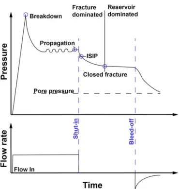
Fig. 3. Illustration of idealized pressure response during an hydraulic
frac-turing test (adapted after9)
(water, oil) and non-Newtonian (polymers) fluids complexify transient pressure analysis. The injection of shear-thinning fluids (i.e., fluid vis-cosity decreases when shear-rates increases) were studied using pressure transient time series.42,43 Laoroongroj et al.44 determined the apparent
fluid viscosity of the shear-thinning fluid and the fluid front radius by TPA techniques.
3. Methods
Our approach follows two steps, which are DFIT and pressure- controlled step analyses. First, we briefly describe the basics of DFIT log-log analyses followed by a summary of the interpretation procedures for pressure-controlled steps.
3.1. DFIT
Fig. 3 presents an idealized pressure and flow rate time series of a typical DFIT. Here, the flow rate is controlled, and variations in injection pressure are monitored uphole. The maximum pressure reached early during the test is referred to as the breakdown pressure and is inter-preted as the moment when a new hydraulic fracture is created. Following the breakdown, the pressure drops due to the fracture prop-agation and associated with fracture volume increase. During fracture propagation, the fluid in the fracture reaches a pressure equilibrium referred to as the propagation pressure. This equilibrium can be influ-enced by fracture connection to natural fractures and leak-off. When the pump is stopped and the injection interval is shut-in, the pressure drops first abruptly, followed by a regime with a slower pressure decay. The fracture dominated regime is replaced by a reservoir dominated regime if most part of the fracture surfaces are in contact. In non-ideal cases, the fracture closes rapidly and the contact pressure aligns with the ISIP. This phenomenon is driven by spatial pressure gradients due to intersection of the hydraulic fractures with pre-existing, natural fractures.
The following interpretation procedure was applied:
1. We inspect a plot with pressure, flow rate versus time to pick the start of injection, shut-in time, and the bleed-off time (Fig. 2).
2. We construct log-log plots of the shut-in data and derivative using the actual shut-in time (see Appendix A.1 for more details) for all tests during refrac cycle RF2 to investigate the influence of test location and fluid rheology (Fig. 4).
3. ‘Barree tangent method’, ‘compliance method’, and ‘variable compliance method’ are presented in Fig. 5b, where only the ‘compliance method’ was systematically applied to evaluate the contact pressure.
4. We construct the plots of the actual shut-in time with dp/dG versus G and G*dp/dG versus G (see Appendix A.2). For convenience, the dp/ dG is always plotted positive. The effective ISIP is extrapolated back to G-time equal to zero if a point of minimum dp/dG prior to contact pressure can be identified (Fig. 5b).
5. The ISIP from the pressure-decay-rate method45 is picked from the
intersection of two linear fits to the p vs dp/dt curve (Fig. 5b). The first line corresponds for most of the tests to a horizontal zero line, and the other line approximates the strong increase of dp/dt, where it does not deviate too far from a straight line.
3.2. Pressure-controlled step tests
The pressure-controlled step tests allow estimating the pressure whereby the fracture in the intersecting of the borehole opens.46 The
objective of these step tests is the characterization of the primary frac-ture in terms of jacking pressure, injectivity, and fracfrac-ture stress-aperfrac-ture relation. The approach adopted here is to combine the injection pressure and uniaxial FBG records.
1. A uniaxial FBG sensor was chosen for further analysis if 1) the Euclidean distance between the FBG-sensor midpoint and the injec-tion interval midpoint was short (i.e. < 5.4 m), and 2) the direcinjec-tion aligned normal to the fracture plane using the plane fit results from the borehole trace and seismic cloud observations.28,47
2. We constructed a plot of the FBG-record (δexp) and the pressure (pexp)
during the step test. The records were down sampled to 1 Hz, syn-chronized, and each pressure step was color-coded. The mean value was calculated from the time interval of the colored section and plotted with flow rate versus pressure as well as strain record versus pressure (Figs. 6 and 7).
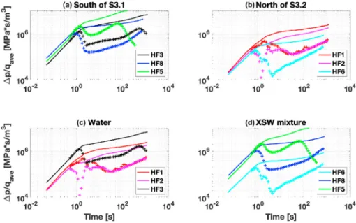
Fig. 4. Pressure response from fracture propagation cycle RF2 for all six experiments normalized by the averaged fluid injection rate from cycle RF2, where the
International Journal of Rock Mechanics and Mining Sciences 135 (2020) 104450 6
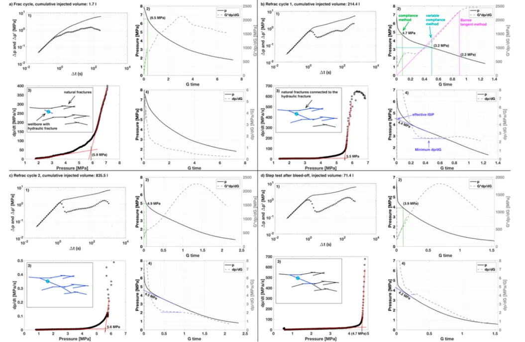
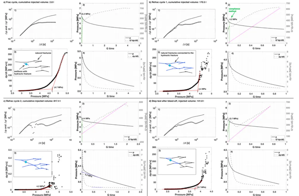
Fig. 5. Evolution of shut-in data from HF3 on p and p′versus t plot (1), dp/dt-pressure (3), G*dp/dG (2) and dp/dG (4) versus G time for a) frac cycle, b) refrac cycle RF1, c) refrac cycle RF2, and d) pressure-controlled
step test (SR). All the different methods presented are used to estimate the ISIP, effective ISIP or contact pressure. The numbers in bracket are not used for the summary Fig. 8. The ‘Barree tangent method’, the ‘variable compliance method’ and the ‘compliance method’ are presented in b), where only the compliance method was systematically applied to all data.
N.
Dutler
et
4. Results and interpretations
4.1. DFIT
4.1.1. Test comparison
Fig. 2c, the transient pressure record of refrac cycle RF2 is presented for the two experiments HF2 and HF8. The propagation pressure at the end of the injection is around 5.2 MPa for test HF2 and 7.7 MPa for test HF8. After shut-in, test HF2 shows a smaller pressure drop compared to test HF8. Then, the transient pressure decays slower for experiment HF2 compared to experiment HF8. In Fig. 4, the transient pressure records are presented for the second fracture propagation cycle RF2 of all the HF tests. The curves (normalized pressure as well as pressure derivative) are grouped according to their location, i.e. (a) south or (b) north of the S3 zone (refer to Fig. 1a) and according to the rheology of the injection
fluid, i.e. (c) water or (d) XSW. We observed similar pressure recovery and derivative among the tests grouped by location with respect to the S3 shear zone. However, strong differences can be seen among the tests with similar fluid rheology. This indicates that fluid rheology may have played a second-order role in the observed fluid pressure propagation.
Fig. 5 presents the evolution of pressure records and their derivatives during actual shut-in time for the HF3 experiment. The sketches (Fig. 5a–d) indicate the connectivity of the hydraulic fracture with the natural, pre-existing fractures. The hydraulic fracture was initiated during the frac cycle (Fig. 5a) with a maximum injection volume of 1.7 L. A rapid pressure decay is observed and the derivative reaches a maximum at 70 s. Both have a concave shape. During refrac cycle RF1 a total of 214.4 l was injected. The pressure record during the subsequent shut-in period (Fig. 5b–1) show a strong slope change at 1 s. The pres-sure record and derivative before 1 s have the same slope, due to
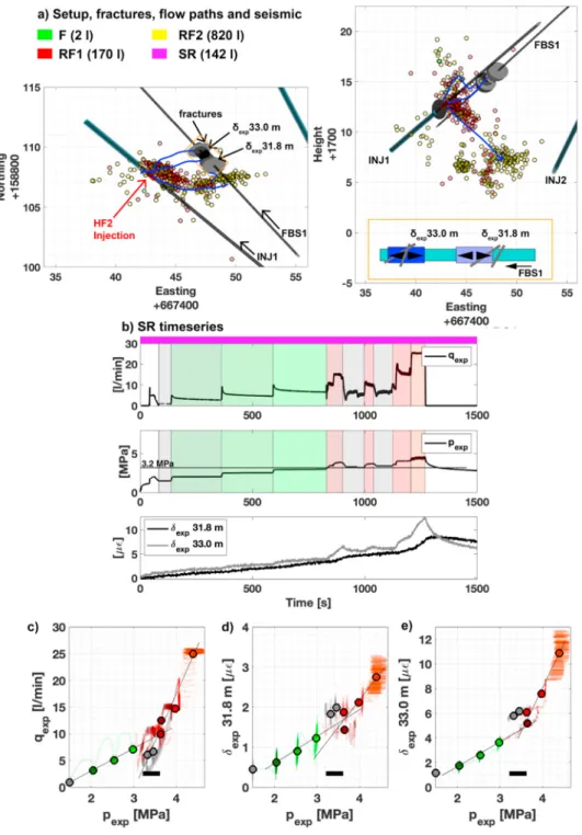
Fig. 6. a) The setup of experiment HF2 in plane
and map view shows the open injection interval (red cylinder), the fractures (grey discs) with the FBG sensors, the seismic cloud depending on jection cycle with the cumulative volume of in-jection fluid in brackets and the flow paths (blue lines). b) The timeseries of the step test is pre-sented for the flow rate, the pressure and two FBG strain records in the surrounding of the in-jection interval and each valid step is colored with red or green. The cross plot is presented to estimate jacking pressure using c) flow rate, d)
δexp at 31.8 m and e) δexp at 33.0 m versus
pres-sure. The circles indicate the mean of the corre-sponding colored sections. (For interpretation of the references to color in this figure legend, the reader is referred to the Web version of this article.)
International Journal of Rock Mechanics and Mining Sciences 135 (2020) 104450
8
wellbore storage. After 1 s, the pressure record and their derivative deviate and fracture network response dominates. The global maximum in the derivative is observed at the end of the shut-in time at 500 s. A similar pressure response is observed during refrac cycle RF2 (Fig. 5c–1), where a cumulative volume of 835.5 l was injected. The global maximum in the derivative is also observed at 500 s. A bleed-off phase was placed in between refrac cycle RF2 and the pressure step test. Therefore, the cumulative injected volume for the step test is only 71.4 l and the pressure does not reach the magnitudes of previous cycles. The derivative reaches the global maximum at 200 s. The bleed-off lead to a depressurization of the rock mass and a new pressurization takes place during the step test. The smaller injection volume leads to a smaller
pressurization front in the rock volume with a dominant leak-off to-wards the natural fractures. This is the reason why the curve of the step test is compressed compared to the previous cycle RF2 (Fig. 5d–1). Data are presented in an identical manner for the experiment HF2 and HF8 in Appendix A.3.
4.1.2. Contact pressure from the G*dp/dG versus G method
Fig. 5b–2) shows the pressure versus G time and the G*dp/dG versus G time with different picking methods. The compliance method is the only method systematically applied during all frac, refrac, and step test cycles. The ‘variable compliance method’ and the ‘Barree tangent method’ are presented for illustrative purposes. The ‘compliance Fig. 7. a) The setup of the experiment HF8 in-
plane and map view shows the open injection interval (red cylinder), the fractures (grey discs) with the FBG sensors, the seismic cloud depend-ing on injection cycle with the cumulative vol-ume of injection fluid in brackets and the flow paths (blue lines). b) The time-series of the step test is presented for the flow rate, the pressure, and two FBG strain records in the surrounding of the injection interval, and each valid step is colored with red or green. The cross plot is pre-sented to estimate jacking pressure using c) flow rate, d) δexp at 12.0 m and e) δexp at 14.0 m versus
pressure. The circles indicate the mean of the corresponding colored sections. (For interpreta-tion of the references to color in this figure legend, the reader is referred to the Web version of this article.)
method’ gives a contact pressure of 4.7 MPa for the refrac cycle RF1 (Fig. 5b–2). The ‘variable compliance method’ and the ‘Barree tangent method’ give values of 3.2 MPa and 2.2 MPa. These two methods always give values below the one estimated from the compliance method. Both methods were generally not suitable due to the short time series as the pick point of both methods come up after the time series. For refrac cycle RF2, the value is 4.9 MPa for the ‘compliance method’ and agrees well with the previous cycle. The value of 6.5 MPa from the frac cycle is bigger than from the refrac cycles and the value from the step-test is smaller with 3.9 MPa.
4.1.3. ISIP from the pressure-decay-rate method
The ISIP from the Pressure-decay-rate method is 5.9 MPa for the frac cycle (Fig. 5a). It is smaller than the value from the ‘compliance method’ for the frac cycle, which is different for the following refrac cycles. The ISIP is 5.5 MPa and 5.6 MPa for the refrac cycles RF1 and RF2, respec-tively. It indicates the biggest magnitude for the refrac cycles compared to the other methods for this experiment. The ISIP is 4.7 MPa and smallest for the step test compared to the previous steps.
4.1.4. Effective ISIP from the dp/dG versus G method
Fig. 5b–4) shows a plot with dp/dG and G-time. The effective ISIP is 4.4 MPa for refrac cycle RF1. The fracture contact is reflected by an increasing slope of dp/dG, but the deviation from Carter leak-off and spatial pressure gradients mask this effect with a decreasing dp/dG slope. The evolution of actual shut-in data of dp/dG versus G-time for the frac cycle (Fig. 5a–4) is monotonically decreasing. For refrac cycle 2
and the step test, we picked the effective ISIP at 4.5 respective 4.2 MPa at the point, where the dp/dG flattens. The interpretation of our ex-periments is labeled as ’lower confidence’ because the ’increase’ in dp/ dG with contact is very weak.
4.2. Pressure-controlled step tests
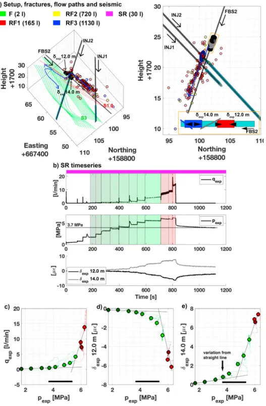
Two examples are presented, one based on a test carried out next to the S1 structure (Fig. 6, HF2) and another one south of the S3 shear zone (Fig. 7, HF8). For both experiments, the field setup including boreholes, injection interval and FBG sensors, main geological domain, fractures, and main flow paths (in blue) are presented. Seismic events are indi-cated by colored circles with a color scheme depending on the respective injection cycle. The biggest injection volume into the rock mass before bleed-off was always achieved in refrac cycle RF2 or RF3. The pressure- controlled step test was executed after a bleed-off phase, and the time series of flow, pressure, and two FBG records are presented in Figs. 6b) and Fig. 7b).
The flow rate and pressure record for HF2 (Fig. 6b) and HF8 (Fig. 7b) is color-coded to account for the different steps with greenish colors if the fracture is closed, reddish colors if the fracture is open and greyish colors if it is unclear if the fracture is open or not. The flow rate versus pressure plot of HF2 (Fig. 6c) shows a bilinear behavior with a jacking pressure of 3.6 MPa using the intersection point after Hartmaier et al.48
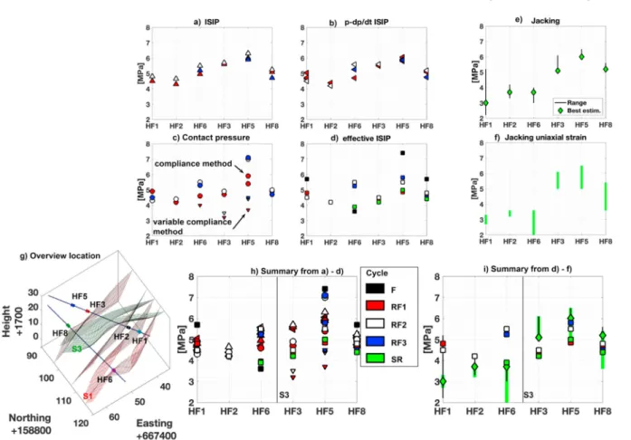
The grey points indicate that flow was unstable. The pressure was decreased and the flow rate dropped, which we assumed that the pres-sure is approaching the jacking prespres-sure. The area of contact of two Fig. 8. Summarizes a) ISIP,28 b) p - dp/dt ISIP, c) contact pressure using G-function, d) effective ISIP, e) jacking pressure28 and f) jacking from uniaxial strain with
color codes for the different injection cycles (see legend). The x-axis indicates the different HF tests with a pseudo-depth starting from the wellbore toe executed test HF1 going up hole to the borehole rim. The overview of each test is indicated in g). A summary of all different picks from the DFIT is presented in h). A summary of the jacking and the effective ISIP is presented in i). (For interpretation of the references to color in this figure legend, the reader is referred to the Web version of this article.)
International Journal of Rock Mechanics and Mining Sciences 135 (2020) 104450
10
fracture surfaces decreases during fracture opening until a critical fracture aperture is reached and the flow rate strongly increases. This starts to happen at about 3.2 MPa. The FBG sensor at 33.0 m is inter-sected by two natural fractures, where one of the fractures is more or less oriented normal to the borehole (Fig. 6a). The FBG sensor at 31.8 m is intersected by a quartz vein. The FBG sensor at 33.0 m indicates a three-time stronger opening component than the one at 31.8 m during the SR test (Fig. 6b). The FBG sensor at 31.8 and 33.0 m has a permanent value of +2.5 respective +2.2 μϵ after the SR test. The jacking pressures estimated from Fig. 6d and e) are 3.6 and 3.5 MPa, respectively, using the intersection point between the two linear fits. The two strain records versus pressure (Fig. 6d and e) present the same characteristics. The solid black bars in Fig. 6c, d, and e) indicate the reliable jacking pressure interval with values ranging between 3.2 and 3.6 MPa.
The flow rate versus pressure plot of HF8 (Fig. 7c) shows a bilinear behavior with a jacking pressure of 5.3 MPa using the intersection point, where we know that the primary fracture is jacked open for the last three steps as the pressure reaches a pressure boundary. The situation looks different considering (Fig. 7e) the strain record at 14.0 m versus pres-sure. The intersection of the two linear fits is around 4.7 MPa. The variation from a straight-line during opening indicates an increase in fracture aperture, meaning a loss of contact between the two rough fracture surfaces. The early deviation from the straight line at 3.7 MPa is related to the decreasing contact area of the fracture surfaces and local fracture stiffness, where the fracture surfaces overall are still in contact. The FBG sensor at 12.0 m is in intact rock prior to the stimulation of HF8. The tensional increase indicates a new hydraulic connection from the injection interval towards this strain sensor. The strain sensor at 14.0 m is intersected by one natural fracture. The curve of Fig. 7e) does not follow a bilinear behavior. It shares similarities in a hyperbolic function. Fig. 7d) shows consistently a similar curve but in a compressional manner. The FBG sensor at 12.0 and 14.0 m has a permanent value of − 4.7 respective +2.3 μϵ after the SR test. The solid black bars in Fig. 7c, d, and e) indicate the reliable jacking pressure interval all applied methods.
4.3. Comparison of methods
As ISIP is generally picked using the tangent to the pressure curve method, it is picked earlier and reflects the upper bound of the minimum principal stress magnitude (Fig. 8a). The ISIP (from 28, the p - dp/dt ISIP
(Fig. 8b), and contact pressure determined using the compliance method on the G-function (Fig. 8c) agree well for a specific refrac cycle. The different refrac cycle shows different trends due to different injection volumes, bleed-off, and injection metrics. For HF1 and HF5, multiple cycles are performed during RF1. For the refrac cycle RF2 for all ex-periments, we notice that the ISIP is between 4.2 and 6.3 MPa. The cumulative injection volume is biggest for the refrac cycle RF2 and the pressurized zone has the largest extension, therefore this cycle is most important to characterize the minimum stress magnitude. The contact pressure determined using the compliance method do range between 4.3 and 7.0 MPa for the refrac cycle RF2 and is similar to the ISIP. In contrast, the ‘variable compliance method’ ranges between 3.5 and 4.4 MPa and gives the smallest magnitudes of all methods.
The effective ISIP (Fig. 8d) using the dp/dG curve shows smaller magnitudes than the other ISIP methods. There is a tendency of bigger variation for the effective ISIP. For the effective ISIP, we see a clear magnitude change for experiment HF6 between frac, refrac, and step test correlated by different injection volumes. The injection of HF6 took place at a pre-existing fracture and during frac cycle, no new fracture was initiated. All the other tests indicate bigger magnitudes during the frac cycle with decreasing effective ISIP for the refrac cycles. The effective ISIP ranges between 4.1 and 5.5 MPa for refrac cycle RF2. If we do not account for experiment HF6, pre-existing fracture in the interval, and HF5, short-cut during the frac cycle to an existing borehole, the effective ISIP ranges only between 4.1 and 4.9 MPa.
The jacking pressure (Fig. 8e) and the jacking from the uniaxial strain record versus pressure
(Fig. 8f) is presented together in Fig. 8i. Both methods indicate a very similar jacking pressure for the primary fracture: the pressure ranges between 1.9 and 5.2 MPa with a mean around 3.5 MPa for the tests executed next to the S1 structure (HF1, HF2, and HF6). The effective ISIP (Fig. 8i) indicate bigger magnitudes compared to the jacking pressure.
For the tests executed south of the S3 domain (HF3, HF5, and HF8), the jacking pressure is between 3.6 and 6.5 MPa (with a mean around 5.0 MPa). The magnitudes of the jacking pressure are similar to slightly above the effective ISIP for these tests. Experiment HF3 shows two different traces of the hydraulic fractures observed in the open wellbore interval, which leads to near-wellbore fracture tortuosity.
5. Discussion
5.1. Transient pressure effects: geology and fluid rheology
The tests analyzed in this study (Fig. 4) are comparable in terms of pressure response and pressure derivative when grouped by spatial location. The test volume consisting of crystalline rock contains natural, pre-existing fractured zones. These zones are responsible for the ma-jority of present-day fluid flow. Depending on the number and orien-tation of fracture sets in the test volume, the pressure response can significantly vary. The hydraulic fracture initialized during the experi-ments located south of the S3 zone (refer to Fig. 1c (S3) and 4a) connect towards the highly fractured S3 zone during the refrac cycles, which dominates the flow field due to the two differently oriented fracture sets (the one developed along shear zones and the one linking the two sub- parallel shear zones). In addition, the true vertical depth from the in-jection location towards the tunnel is only 15 m. Pressure diffuses along the pre-existing fractures towards the atmospheric tunnel boundaries and may lead to faster fracture surface contact than experiments per-formed north of the S3 zone. The experiments perper-formed next to the S1 zone (refer to Fig. 4b and north of the S3 zone) indicate a connection from the hydraulic fracture towards the fracture set associated with the S1 zone, which is further disconnected to the tunnel (Fig. 1c). This single fracture set and the increase in true vertical depth of ~30 m from the tunnels to the injection location are captured by the pressure and de-rivative response.
In contrast, the similarities disappear if the tests are grouped by injection-fluid rheology (Fig. 4c and d). The pressure time series from RF1 and RF2 is potentially affected by the rheology with a maximal pressure increase of 0.5 MPa.28 The effect on the ISIP is potentially
smaller depending on the method to determine the ISIP and is more likely dominated by the injection volume and leak-off. The change in fluid rheology does not appear to dominate the pressure response, but the change from XSW to water during the additional flushing cycle can nevertheless influence the response. First, the water will push the XSW farther into the fracture system. Then, given the initially-low viscosity contrast, the two fluids are partly miscible and the XSW is likely held back in the irregularities of the rough fractures. Nevertheless, the vis-cosity contrast of approximately 30 times in our case is most likely insufficient to strongly influence the pressure response. However, it is still unclear, how such contrasts affect the leak-off from the hydraulic fracture towards the natural, pre-existing fractures. Our data do there-fore not allow to quantify the influence on fracture leak-off.
5.2. Best estimate of the minimum principal stress magnitude
Higher stress magnitudes are observed for the effective ISIP (e.g., Fig. 8d) during the frac cycle compared to the following refrac cycles. No data points are given, if the dp/dG curve monotonically decreases. The ISIP from dp/dt, the contact pressure from G-function and effective ISIP from the refrac cycles do not show a correlation with the injection N. Dutler et al.
volume (Fig. 8b–d). The following bleed-off phase leads to strong pres-sure release in the rock mass. This changes the system behavior and allows to characterize the initialized hydraulic fracture intersecting the open injection interval with the shortcoming that the assumption of uniform pressure in the fracture is not valid. For these reasons, only the refrac cycles were used to calculate the ISIP (σRFISIP) and effective ISIP
(σRFeff. ISIP). The mean and standard deviation of all refrac cycles together
for each experiment are presented in Table 2 and Fig. 9a. Besides the mean and standard deviation of the jacking pressure (σSRJP) is calculated
from the flow rate versus pressure (Fig. 8e) and two uniaxial strain versus pressure (Fig. 8f) results for each experiment.
The ISIP for all six experiments is 4.81±0.38 MPa (Fig. 9b). It in-dicates the pressure that is measured in the wellbore. The effective ISIP is 4.49±0.22 MPa (Fig. 9b). The effective ISIP is smaller than the ISIP measured in the wellbore, as it is picked later and should be a better estimate for the minimum principal stress at the fracture tip. The dif-ference of the two values are rather small for our crystalline rock with natural, pre-existing fractures. McClure et al.16 analyzed over 30 field DFIT from shale and indicated that the minimum principal stress is slightly below the contact pressure, which was identified from a plot of dp/dG or relative system stiffness. Our observations from the plot of dp/dG (e.g., Figs. 5, 11 and 12) is often monotonically decreasing, which was identified to be related by the hydraulic fracture intersecting highly permeable natural, pre-existing fractures. The fracture closes quickly and the reversible mechanical strain released due to shut-in might develop spatial pressure gradients. The relative stiffness plot16 assumes
a uniform pressure everywhere in the fracture and McClure et al.16
recommend a rapid closure interpretation under this conditions. Therefore, we did not use a relative stiffness plot in our analysis.
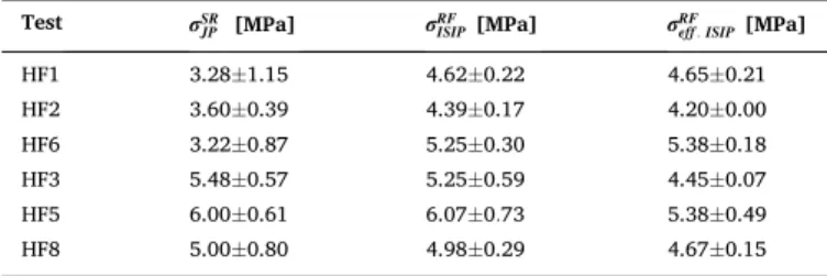
Experiments HF1, HF2, and HF6 executed next to the S1 structure (Fig. 9c) indicate similar jacking pressure with a magnitude of 3.37±0.20 MPa (Fig. 9b), proving an estimate of the primary fracture opening. This pressure is around 1.1 MPa smaller than the effective ISIP. The mean and standard deviation of the jacking pressure is 5.49±0.50
MPa (Fig. 9b) for the experiments HF3, HF5, and HF8 executed south of the S3 structure (Fig. 9c). The jacking pressure for the experiments executed south of the S3 structure is around 1.0 MPa bigger than the one from the effective ISIP. It is likely that the magnitudes of the jacking pressure from the pressure-controlled step tests overestimate the mini-mum principal stress magnitude for fracture tortuosity near the well-bore. It is unlikely, that the jacking pressure is below the effective ISIP, which might be an indication for shear reactivation. Therefore, we conclude that effective ISIP gives the best estimate for the minimum principal stress magnitude due to small differences between different experiments (Table 3).
5.3. Implication for the stress field
The pole points of the traces of the hydraulic fractures observed in the open wellbore interval (here: HF traces) and the seismic plane fits from Dutler et al.28 and Villiger et al.47 are presented in a
lower-hemisphere stereonet (Fig. 9d). All pole points of the HF traces (diamonds) indicate a consistent orientation. In addition, the seismic plane fit for HF5 and one cluster of HF2 (during the early time of frac-turing) are oriented in a similar manner. The trend and plunge for the minimum principal stress was assumed to correspond to the HF traces. All observed HF traces were used to calculate49,50 the Fischer
distribu-tion giving the trend and plunge for σ3 in Table 3. The maximum prin-cipal stress magnitude, trend, and plunge was adapted from Krietsch et al.31 Krietsch et al.31 applied two stress relief methods (CSIRO HI and
USBM cells) in three different oriented boreholes to constrain σ1 using transverse isotropic rock model. Major and minor principal stress was successfully checked for orthogonality. The limiting pressure observed during the high-pressure injection is 5.4 MPa and 6.8 MPa (see Fig. 4a in Dutler et al.28) for the experiments north (e.g., HF2) and south of S3 (e.
g., HF8). We assume that, this overpressure is able to reactivate the corresponding fractures leading to the overall seismic plane fit in Fig. 10c. This allowed us to derive the magnitude of σ2 as 6.7 MPa. The
perturbed stress state was derived for the nearfield towards the S3 structure, where the fracture density increases.31 This perturbation leads
to a switched position between σ2 and σ3, where the magnitude has to be
Table 2
Summary of magnitudes from the different minimum principal stress estimates from the refrac cycles and step tests (see Fig. 9a).
Test σSR
JP [MPa] σRFISIP [MPa] σRFeff . ISIP [MPa]
HF1 3.28±1.15 4.62±0.22 4.65±0.21 HF2 3.60±0.39 4.39±0.17 4.20±0.00 HF6 3.22±0.87 5.25±0.30 5.38±0.18 HF3 5.48±0.57 5.25±0.59 4.45±0.07 HF5 6.00±0.61 6.07±0.73 5.38±0.49 HF8 5.00±0.80 4.98±0.29 4.67±0.15
Fig. 9. a) Summarizes the results from Fig. 8 for the mean and standard deviation of the jacking pressure (σSRJP), the ISIP (σRFISIP) and effective ISIP (σRFeff. ISIP) for each experiment and b) the mean and standard deviation over all experiments without experiment HF6 (due to the pre-existing fracture in the interval). c) Sketch from the location of the experiments relative to the fractured zones. d) The lower stereonet presents the pole points of the HF traces (diamonds) from Dutler et al.28 and seismic
plane fit (squares) from Villiger et al.47 and Dutler et al.28
Table 3
Summary of magnitudes, trend, and plunge from the three stress components used in this study.
Stress component Magnitude [MPa] Trend [◦] Plunge [◦]
σ1 13.1 104 39
σ2 6.7 313 46
International Journal of Rock Mechanics and Mining Sciences 135 (2020) 104450
12
in a similar range.
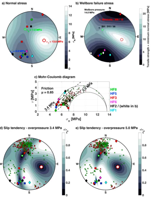
The stress tensor (Table 3) is presented in the lower-hemisphere stereonet with the normal stress component (Fig. 10a). The HF traces (diamonds) and seismic plane fits (squares) are located in the part indicating small normal stress magnitudes.
Fig. 10b is showing the wellbore failure stress distribution containing the distribution of the minimum of such wellbore failure stress and the anisotropic tensile strength. The wellbore failure stress uses an arbi-trarily virtual plane intersecting the wellbore (BH: 310/56◦) and the resolved normal stress acting on the plane was calculated along the plane’s trace on the wellbore wall using the Kirsch solution. The anisotropic tensile strength varies between 5.6 and 14.0 MPa, which is aligned with the foliation plane (schistosity: 330/15◦). Fig. 10b shows only one injection borehole orientation, the other borehole is oriented similar and has been omitted for the sake of simplicity. The injected fluid pressurizes the wellbore. A fracture can be generated through a plane when its wellbore failure stress becomes zero or negative. The moment when the wellbore pressure is 14.0 MPa is shown in Fig. 10b, which was determined as the minimum value by increasing the wellbore pressure and so decreasing the wellbore failure stress on most of the observed HF traces to zero. The tensile strength on the orientations of the wellbore
traces are around 13.0–14.0 MPa, based on the relative orientations from the foliation plane. HF traces with a positive wellbore failure stress do only fail at higher wellbore pressure. The observed wellbore failure pressure was minimal with 14.0 MPa and ranged between 14.0 and 21.0 MPa (called formation break down pressure in Ref. 28), which agrees well as seven of eight HF traces fail.
Hydraulic fracturing theory dictates that the plane of a hydraulic fracture is oriented perpendicular to the minimum principal stress. Most likely, this was achieved at the early stage of fracturing (frac cycle and refrac RF1). A small slip tendency is indicated for the wellbore trace of HF3, HF5, and HF8 and the seismic cloud of HF2 next to σ3 (Fig. 10d +
e). With additional injection volume and flow rate, the hydraulic frac-ture grows and interconnects to natural, pre-existing fracfrac-tures and leaks more and more fluid towards them. Consequently, the seismic cloud starts to change the orientation resulting in a seismic plane fit of HF8, HF3, and HF2 oriented towards N-aligning with the pre-existing, natural fracture set K1 (red and green triangles). A second red square (HF3) is located next to the other fracture set K2 associated with the S3 structure, indicating a low slip tendency. The most substantial slip tendency is associated with the HF traces from experiment HF1, HF2, and HF6. The shear-stress ranges between 2.0 and 3.4 MPa (Fig. 10c). It is evident Fig. 10. a) The normal stress under the given stress
state and b) wellbore failure stress consisting of the Kirsch solution for the given borehole direction (BH) and the anisotropic tensile strength from the shistos-ity at a given wellbore pressure of 14.0 MPa. c) The Mohr-Coulomb diagram is calculated from stress field given by Table 3. The Mohr circles include the hydro- static pressure of 0.5 MPa. The failure envelopes assuming a friction coefficient of 0.85, no cohesion and overpressure of 3.4, and 5.0 MPa. The diamonds and the squares are the pole points of the wellbore trace and seismic plane fit (Fig. 9). The red and green triangles are the natural fractures related to the S1 and S3 structure (Fig. 1). The slip tendency is pre-sented for an overpressure of d) 3.4 MPa and e) 5.0 MPa. (For interpretation of the references to color in this figure legend, the reader is referred to the Web version of this article.)
International Journal of Rock Mechanics and Mining Sciences 135 (2020) 104450 13
Fig. 11. Evolution of shut-in data from HF2 on p and p′versus t plot (1), dp/dt-pressure (3), G*dp/dG (2) and dp/dG (4) versus G time for a) frac cycle, b) refrac cycle RF1, c) refrac cycle RF2, and d) pressure-controlled
step test (SR). All the different methods presented are used to estimate the ISIP, effective ISIP or contact pressure. The numbers in bracket are not used for the summary Fig. 8. The contact pressure on G-function and the applied methods are presented in Fig. 5b.
Dutler
et
International Journal of Rock Mechanics and Mining Sciences 135 (2020) 104450 14
Fig. 12. Evolution of shut-in data from HF8 on p and p′versus t plot (1), dp/dt-pressure (3), G*dp/dG (2) and dp/dG (4) versus G time for a) frac cycle, b) refrac cycle RF1, c) refrac cycle RF2, and d) refrac cycle RF3.
All the different methods presented are used to estimate the ISIP, effective ISIP or contact pressure. The numbers in bracket are not used for the summary Fig. 8. The contact pressure on G-function and the applied methods are presented in Fig. 5b.
N.
Dutler
et
from an inspection of Fig. 10 that slip occurs between 3.0 and 4.0 MPa overpressure (evidence in Fig. 6c). Therefore, the jacking pressure (Fig. 9a) of these experiments indicate shear dilation and not fracture opening. In comparison, the effective ISIP and ISIP (Fig. 9a) was similar for all experiments with two exceptions (HF5 and HF6).
The experiment HF3, HF5, and HF8 (Fig. 9c) indicate a small slip tendency. The maximum shear stress is around 1.5 MPa. The over-pressure needed to open or reactivate the fractures in shear is between 3.5 and 5.5 MPa. The jacking pressure of these experiments indicates fracture opening, with a tendency to overestimate σ3 due to near- wellbore tortuosity. Experiment HF5 shows tendential bigger magni-tudes for σ3. This is probably related to hydraulic short-cut towards an
unpacked geophysical borehole during the frac cycle and/or local stress effects. Most of the fractures related to the S1 (red triangles) and S3 (green triangles) structures can be reactivated with an overpressure of 5.0 MPa.
6. Conclusions
The DFIT methods: ISIP, p-dp/dt ISIP, and the contact pressure from G-function allow to pick pressure consistently in the crystalline rock mass. The ‘compliance method’ for the G-function reproduced similar values as the ISIP from other methods. The overall ISIP is 4.81±0.38 MPa and indicates the pressure in the open wellbore interval. These selected ISIPs do yield slightly larger pressure magnitudes than the picked effective ISIP from the dp/dG curve. It is assumed that the effective ISIP to be a better estimate of the minimum principal stress magnitude referred to the fracture tip. The overall effective ISIP is 4.49±0.22 MPa. The jacking pressure for the experiments executed South of the S3 structure is 5.49±0.50 MPa from the pressure-controlled step test. The proximity to the S3 structure and the complex geological structure led to near-wellbore tortuosity and heterogeneous stress ef-fects masking the jacking pressure. In comparison, the tests executed North of the S3 structure show smaller jacking pressure than effective ISIP.
A new method was introduced to estimate the jacking pressure from uniaxial strain records versus pressure plot. The values agree with the observations from the jacking pressure from the flow versus pressure plot. The permanent changes in strain are indicative of shear dislocation as well as fracture opening during the pressure-controlled step tests. One experiment presented had a jacking pressure below the effective ISIP,
and another experiment vice versa. The slip-tendency analysis showed that the jacking pressure below the effective ISIP is related to shear dislocation and not indicative of the fracture opening.
The orientation of σ3 was estimated from the hydraulic fracture intersecting the wellbore with the assumption that the maximum prin-cipal stress axis is stable in orientation. The minimum prinprin-cipal stress magnitude of 4.49±0.22 MPa was estimated from the DFIT methods using effective ISIP. The orientation of σ2 is aligned next to the fracture system K1. The difference in magnitude of σ2 and σ3 is small, such that they can switch place. Besides, the hydraulic fracture connects to the pre-existing, natural fracture set K1 and forces the fluid to follow this fracture set, indicating possible shear slip. The newly derived stress tensor for the HF experiments is σ1 =13.1 MPa (104/39◦), σ
2 =6.7 MPa (313/46◦), and σ
3 =4.5 MPa (206/19◦).
Declaration of competing interest
The authors declare that they have no known competing financial interests or personal relationships that could have appeared to influence the work reported in this paper.
Acknowledgement
The ISC is a project of the Deep Underground Laboratory at ETH Zurich, established by the Swiss Competence Center for Energy Research - Supply of Electricity (SCCER-SoE) with the support of Innosuisse. Funding for the ISC project was provided by the ETH Foundation with grants from Shell and EWZ and by the Swiss Federal Office of Energy through a P&D grant. Nathan Dutler is supported by SNF grant 200021–165677, and Hannes Krietsch is supported by SNF grant 200021–169178. The authors thank Gerd Klee and his staff from MeSy Solexperts, Bochum (Germany) for their good collaboration and helpful discussions. The Grimsel Test Site is operated by Nagra, the National Cooperative for the Disposal of Radioactive Waste. We are indebted to Nagra for hosting the ISC experiment in their GTS facility and to the Nagra technical staff for onsite support. The authors acknowledge the editor Jian Zhao and five anonym reviewers for the constructive com-ments that substantially improved the manuscript. Besides, the authors gratefully acknowledge Mark McClure for his thoughts and suggestions on the applied methods.
Appendix D. Supplementary data
Supplementary data to this article can be found online at https://doi.org/10.1016/j.ijrmms.2020.104450.
Appendix A.1. Change in pressure and derivative
The change in pressure is defined by
Δp(t) = p(t = tshut− in) − p(t) for t ∈ (tshut− in,tend] (A.1)
All derivatives used for the diagnostic plots in this paper correspond to first-order, logarithmic time derivatives.51 The involved signal was
resampled with a spline interpolation at a fixed number of time intervals regularly spaced in a logarithmic scale.52 The derivatives were taken with
respect to actual shut-in time, ta =t/tp, t is the time since shut-in, tp is the duration of injection taking place prior shut-in.
Δp′(t) =dΔp dlnta
=ta dΔp
dta (A.2)
Appendix A.2. G-function
The G-time (or G-function) is a dimensionless function relating to shut-in time with the duration of the injection. It allows estimating the minimum principal stress, pore pressure, and permeability10 with the assumption that the cumulative leak-off after shut-in is linearly proportional to G-time. The
International Journal of Rock Mechanics and Mining Sciences 135 (2020) 104450 16 G(ta,α) = 4 π[g(ta,α) − g(0,α)] (A.3) with g(ta,α=1 ) = 4 3 [ (1 + ta)1.5− t1.5a ] (A.4) g(ta,α=0.5 ) = (1 + ta)sin−1(1 + ta) −0.5+ t0.5 a (A.5)
where tais the actual shut-in time and α is the power law exponent for fracture growth. The G-function depends weakly on α and the reasonable bounds
of α are between 0.5 and 1.0.10 The higher bound is for low leak-off with high efficiency fracturing, where the fracture area depends linearly on time. We choose α=1 for our tests in low permeability rock. The choice of α does not affect the method of picking contact pressure.
The G-function is derived based on the assumption of Carter leak-off. The analytical solution of the 1D fluid flow leak-off from a fracture into an infinite homogeneous and isotropic porous medium is described by a 1D seepage model53:
∂p ∂t=C
∂2 p
∂x2 (A.6)
with x > 0, t > 0. It corresponds to a simple 1D diffusion model with a conductivity C. The initial and boundary conditions are p(0, t) = pinj for t > 0,
p(∞, t) = pformation for t > 0 and p(x, 0) = pformation for x ≥ 0. Carter’s leak-off equation links the fluid velocity vL in the hydraulic fracture with Carter’s
leak-off coefficient cL: vL= cL ̅̅̅̅̅̅̅̅̅̅̅̅̅̅̅̅̅̅̅̅ t − tshut− in √ (A.7)
where the spatial derivation of the solution to the 1D seepage model leads to the leak-off velocity. The solution to the 1D seepage model is given by:
p(x, t) =(pinj− pformation ) erfc ( x 2√̅̅̅̅̅Ct ) +pformation (A.8)
Relying on the assumption that the cumulative leak-off after shut-in is proportional to G-time, the derivative of the cumulative leak-off with respect to G-time is equal to a constant. The pressure versus G-time plot should form a straight line. It also means that the fracture stiffness before contact is constant, as well as the total system storage, which is truly an ideal theoretical case.
dp dG= 1 Ct dV dG=constant (A.9)
Appendix A.3. DFIT from experiment HF2 and HF8
Figs. 11 and 12 present the evolution of pressure records and their derivatives during actual shut-in time for the HF2 and HF8 experiment. The figures are presented for comparison and completeness to give an overview of the DFIT before the pressure-controlled step test (i.e. Figs. 6 and 7). All applied methods are presented in the method section and their color code can be found in Fig. 5b.
References
1 Theis CV. The relation between the lowering of the Piezometric surface and the rate and duration of discharge of a well using groundwater storage. Eos, Trans Am
Geophys Union. 1935;16(2):519–524. https://doi.org/10.1029/TR016i002p00519. 2 Matthews CS, Russell DG. Pressure Buildup and Flow Tests in Wells. 130–133. Society
of Petroleum Engineers of AIME; 1967. Retrieved from http://store.spe.org/Pressur
e-Buildup-and-Flow-Tests-in-Wells-P49.aspx.
3 Zarrouk SJ, McLean K. Geothermal Well Test Analysis. London: Elsevier; 2019. Katie
Hammon.
4 Warren JE, Root PJ. The behavior of naturally fractured reservoirs. Soc Petrol Eng J. 1963;3(3):245–255. https://doi.org/10.2118/426-PA.
5 Barker JA. A generalized radial flow model for hydraulic tests in fractured rock.
Water Resour Res. 1988;24(10):1796–1804. https://doi.org/10.1029/
WR024i010p01796.
6 Acuna JA, Yortsos YC. Application of fractal geometry to the study of networks of fractures and their pressure transient. Water Resour Res. 1995;31(3):527–540.
https://doi.org/10.1029/94WR02260.
7 Chang J, Yortsos YC. Pressure-Transient Analysis of Fractal Reservoirs. SPE Formation
Evaluation; 1990:31–38 (March).
8 Economides M, Nolte K. Reservoir Stimulation (3th Editio). Chichester: Wiley; 2000.
9 Schmitt DR, Haimson B. Hydraulic fracturing stress measurements in deep holes. In: Rock
Mechanics and Engineering. 1. CRC Press; 2017:183–225. https://doi.org/10.1201/
9781315364261. Principles.
10 Nolte KG. Determination of fracture parameters from fracturing pressure decline. In:
SPE Annual Technical Conference and Exhibition. 1979:SPE8341. https://doi.org/
10.2118/8341-MS. Las Vegas, Nevada. Retrieved from.
11 Barree RD, Barree VL, Llc A, Craig DP. Holistic fracture diagnostics. SPE rocky oil & gas technology symposium. https://doi.org/10.2118/107877-PA; 2007.
12 Jung H, Sharma MM, Cramer DD, Oakes S, McClure MW. Re-examining interpretations of non-ideal behavior during diagnostic fracture injection tests.
J Petrol Sci Eng. 2016;145:114–136. https://doi.org/10.1016/j.petrol.2016.03.016. 13 McClure MW, Blyton CAJ, Jung H, Sharma MM. The effect of changing fracture
compliance on pressure transient behavior during diagnostic fracture injection tests. In: SPE Annual Technical Conference and Exhibition. 2014. https://doi.org/10.2118/
170956-MS.
14 McClure MW, Jung H, Cramer DD, Sharma MM. The fracture-compliance method for picking closure pressure from diagnostic fracture-injection tests (see associated supplementary discussion/reply). SPE J. 2016;21(4):1321–1339. https://doi.org/
10.2118/179725-PA.
15 Wang H, Sharma MM. Determine in-situ stress and characterize complex fractures in naturally fractured reservoirs from diagnostic fracture injection tests. Rock Mech
Rock Eng. 2019;52(12):5025–5045. https://doi.org/10.1007/s00603-019-01793-w. 16 McClure M, Bammidi V, Cipolla C, et al. A collaborative study on DFIT
interpretation: integrating modeling, field data, and analytical techniques. In:
Proceedings of the 7th Unconventional Resources Technology Conference. Tulsa, OK,
USA: American Association of Petroleum Geologists; 2019:1–39. https://doi.org/
10.15530/urtec-2019-123.
17 Rutqvist J, Stephansson O. A cyclic hydraulic jacking test to determine the in situ stress normal to a fracture. Int J Rock Mech Mining Sci Geomech. 1996;33(7):695–711.
https://doi.org/10.1016/0148-9062(96)00013-7.
18 Bandis SC, Lumsden AC, Barton NR. Fundamentals of rock joint deformation. Int J
Rock Mech Mining. 1983. https://doi.org/10.1016/0148-9062(83)90595-8.
19 Goodman R, Taylor R, Brekke T. A model for the mechanics of jointed rock. Soil
Mechanics and Foundations Division ASCE. 1968;94(SM3):367–659.