HAL Id: hal-02137968
https://hal.archives-ouvertes.fr/hal-02137968v4
Submitted on 13 Mar 2020
HAL is a multi-disciplinary open access
archive for the deposit and dissemination of
sci-entific research documents, whether they are
pub-lished or not. The documents may come from
teaching and research institutions in France or
abroad, or from public or private research centers.
L’archive ouverte pluridisciplinaire HAL, est
destinée au dépôt et à la diffusion de documents
scientifiques de niveau recherche, publiés ou non,
émanant des établissements d’enseignement et de
recherche français ou étrangers, des laboratoires
publics ou privés.
floating-point operations using round-to-nearest
ties-to-even arithmetic
Sylvie Boldo, Christoph Lauter, Jean-Michel Muller
To cite this version:
Sylvie Boldo, Christoph Lauter, Jean-Michel Muller. Emulating round-to-nearest ties-to-zero
”aug-mented” floating-point operations using round-to-nearest ties-to-even arithmetic. IEEE Transactions
on Computers, Institute of Electrical and Electronics Engineers, In press, �10.1109/TC.2020.3002702�.
�hal-02137968v4�
Emulating Round-to-Nearest Ties-to-Zero
“Augmented” Floating-Point Operations Using
Round-to-Nearest Ties-to-Even Arithmetic
Sylvie Boldo
*, Christoph Lauter
†, Jean-Michel Muller
‡*
Université Paris-Saclay, Univ. Paris-Sud, CNRS, Inria, Laboratoire de recherche en informatique, 91405 Orsay,
France
†University of Alaska Anchorage, College of Engineering, Computer Science Department, Anchorage,
AK, USA
‡Univ Lyon, CNRS, ENS de Lyon, Inria, Université Claude Bernard Lyon 1, LIP UMR 5668, F-69007
Lyon, France
Abstract—The 2019 version of the IEEE 754 Standard for Floating-Point Arithmetic recommends that new “augmented” operations should be provided for the binary formats. These operations use a new “rounding direction”: round-to-nearest ties-to-zero. We show how they can be implemented using the currently available operations, using round-to-nearest ties-to-even with a partial formal proof of correctness.
Keywords. Floating-point arithmetic, Numerical repro-ducibility, Rounding error analysis, Error-free transforms, Rounding mode, Formal proof.
I. INTRODUCTION AND NOTATION
The new IEEE 754-2019 Standard for Floating-Point (FP) Arithmetic [8] supersedes the 2008 version. It recommends that new “augmented” operations should be provided for the binary formats (see [15] for history and motivation). These operations are called augmentedAddition, augmentedSub-traction, and augmentedMultiplication. They use a new “rounding direction”: round-to-nearest ties-to-zero. The reason behind this recommendation is that these operations would significantly help to implement reproducible summation and dot product, using an algorithm due to Demmel, Ahrens, and NGuyen [5]. Obtaining very fast reproducible summation with that algorithm may require a direct hardware implementation of these operations. However, having these operations avail-able on common processors will certainly take time, and they may not be available on all platforms. The purpose of this paper is to show that, in the meantime, one can emulate these operations with conventional FP operations (with the usual round-to-nearest ties-to-even rounding direction), with reasonable efficiency. In this paper, we present the first pro-posed emulation algorithms, with proof of their correctness and experimental results. This allows, for instance, the design of programs that use these operations, and that will be ready for use with full efficiency as soon as the augmented operations are available in hardware. Also, when these operations are available in hardware on some systems, this will improve the portability of programs using these operations by allowing them to still work (with degraded performance, however) on other systems.
In the following, we assume radix-2, precision-𝑝 floating-point arithmetic [13]. The minimum floating-floating-point exponent is
𝑒min< 0 and the maximum exponent is 𝑒max. A floating-point
number is a number of the form
𝑥 = 𝑀𝑥× 2𝑒𝑥−𝑝+1, (1)
where
𝑀𝑥 is an integer satisfying |𝑀𝑥| ≤ 2𝑝− 1, (2)
and
𝑒min≤ 𝑒𝑥≤ 𝑒max. (3)
If |𝑀𝑥| is maximum under the constraints (1), (2), and (3),
then 𝑒𝑥is the floating-point exponent of 𝑥. The number 2𝑒minis
the smallest positive normal number (a FP number of absolute value less than 2𝑒minis called subnormal), and 2𝑒min−𝑝+1is the
smallest positive FP number. The largest positive FP number is
Ω = (2 − 2−𝑝+1) · 2𝑒max.
We will assume
3𝑝 ≤ 𝑒max+ 1, (4)
which is satisfied by all binary formats of the IEEE 754 Stan-dard, with the exception of binary16 (which is an interchange formatbut not a basic format [8]). The usual round-to-nearest, ties-to-even function (which is the default in the IEEE-754 Standard) will be noted RN𝑒. We recall its definition [8]:
RN𝑒(𝑡) (where 𝑡 is a real number) is the
point number nearest to 𝑡. If the two nearest floating-point numbers bracketing 𝑡 are equally near, RN𝑒(𝑡)
is the one whose least significant bit is zero. If |𝑡| ≥ Ω + 2𝑒max−𝑝then RN
𝑒(𝑡) = ∞, with the same
sign as 𝑡.
We will also assume that an FMA (fused multiply-add) instruction is available. This is the case on all recent FP units. As said above, the new recommended operations use a new “rounding direction”: round-to-nearest ties-to-zero. It corre-sponds to the rounding function RN0 defined as follows [8]:
RN0(𝑡) (where 𝑡 is a real number) is the
point number nearest 𝑡. If the two nearest floating-point numbers bracketing 𝑡 are equally near, RN0(𝑡) is the one with smaller magnitude. If
|𝑡| > Ω + 2𝑒max−𝑝then RN
0(𝑡) = ∞, with the same
This is illustrated in Fig. 1. As one can infer from the defini-tions, RN𝑒(𝑡) and RN0(𝑡) can differ in only two circumstances
(called halfway cases): when 𝑡 is halfway between two consec-utive floating-point numbers, and when 𝑡 = ±(Ω + 2𝑒max−𝑝).
0 +∞ RN0(𝑥) = RN𝑒(𝑥) 𝑥 𝑦 RN0(𝑦) RN𝑒(𝑦) 100100 100101 100110 100111 101000
Fig. 1: Round-to-nearest ties-to-zero (assuming we are in the positive range). Number 𝑥 is rounded to the (unique) FP number nearest to 𝑥. Number 𝑦 is a halfway case: it is exactly halfway between two consecutive FP numbers: it is rounded to the one that has the smallest magnitude.
The augmented operations are required to behave as fol-lows [8], [15]:
∙ augmentedAddition(𝑥, 𝑦) delivers (𝑎0, 𝑏0) such that
𝑎0 = RN0(𝑥 + 𝑦) and, when 𝑎0 ∈ {±∞, NaN},/
𝑏0= (𝑥+𝑦)−𝑎0. When 𝑏0= 0, it is required to have the
same sign as 𝑎0. One easily shows that 𝑏0is a FP number.
For special rules when 𝑎0∈ {±∞, NaN}, see [15]; ∙ augmentedSubtraction(𝑥, 𝑦) is exactly the same as
augmentedAddition(𝑥, −𝑦), so we will not discuss that operation further;
∙ augmentedMultiplication(𝑥, 𝑦) delivers (𝑎0, 𝑏0) such
that 𝑎0 = RN0(𝑥 · 𝑦) and, where 𝑎0 ∈ {±∞, NaN},/
𝑏0 = RN0((𝑥 · 𝑦) − 𝑎0). When (𝑥 · 𝑦) − 𝑎0 = 0, the
floating-point number 𝑏0 (equal to zero) is required to
have the same sign as 𝑎0. Note that in some corner cases
(an example is given in Section IV-A), 𝑏0 may differ
from (𝑥 · 𝑦) − 𝑎0 (in other words, (𝑥 · 𝑦) − 𝑎0 is not
always a floating-point number). Again, rules for handling infinities, NaNs and the signs of zeroes are given in [8], [15].
Because of the different rounding function, these augmented operations differ from the well-known Fast2Sum, 2Sum, and Fast2Mult algorithms (Algorithms 1, 2 and 3 below). As said above, the goal of this paper is to show that one can implement these augmented operations just by using rounded-to-nearest ties-to-even FP operations and with reasonable efficiency on a system compliant with IEEE 754-2008.
Let 𝑡 be the exact sum 𝑥 + 𝑦 (if we consider implementing augmentedAddition) or the exact product 𝑥 · 𝑦 for augment-edMultiplication). To implement the augmented operations, in the general case (i.e., the sum or product does not overflow, and in the case of augmentedMultiplication, 𝑥 and 𝑦 satisfy the requirements of Lemma 2 below), we first use the clas-sical Fast2Sum, 2Sum, or Fast2Mult algorithms to generate two FP numbers 𝑎𝑒 and 𝑏𝑒 such that 𝑎𝑒 = RN𝑒(𝑡) and
𝑏𝑒 = 𝑡 − 𝑎𝑒. We explain how augmentedAddition(𝑥, 𝑦) and
augmentedMultiplication(𝑥, 𝑦) can be obtained from 𝑎𝑒and 𝑏𝑒
in Sections III and IV, respectively, using a “recomposition” algorithm presented in Section II.
In the following, we need to use a definition inspired from Harrison’s definition [6] of function ulp (“unit in the last
place”). If 𝑥 is a floating-point number different from −Ω, first define pred(𝑥) as the floating-point predecessor of 𝑥, i.e., the largest floating-point number < 𝑥. We define ulp𝐻(𝑥) as follows.
Definition 1 (Harrison’s ulp). If 𝑥 is a floating-point number, thenulp𝐻(𝑥) is
|𝑥| − pred (|𝑥|) .
Notation ulp𝐻is to avoid confusion with the usual definition of function ulp. The usual ulp and function ulp𝐻 differ at powers of 2, except in the subnormal domain. For instance, ulp(1) = 2−𝑝+1, whereas ulp𝐻(1) = 2−𝑝. One easily checks that if |𝑡| is not a power of 2, then ulp(𝑡) = ulp𝐻(𝑡), and if |𝑡| = 2𝑘, then ulp(𝑡) = 2𝑘−𝑝+1
= 2ulp𝐻(𝑡), except in the
subnormal range where ulp(𝑡) = ulp𝐻(𝑡) = 2𝑒min−𝑝+1.
The reason for choosing function ulp𝐻 instead of function ulp is twofold:
∙ if 𝑡 > 0 is a real number, each time RN0(𝑡) differs from
RN𝑒(𝑡), RN0(𝑡) will be the floating-point predecessor
of RN𝑒(𝑡), because RN0(𝑡) ̸= RN𝑒(𝑡) implies that 𝑡
is what we call a “halfway case” in Section II: it is exactly halfway between two consecutive floating-point numbers, and in that case, RN0(𝑡) is the one of these
two FP numbers which is closest to zero and RN𝑒(𝑡) is
the other one. Hence, in these cases, to obtain RN0(𝑡)
we will have to subtract from RN𝑒(𝑡) a number which
is exactly ulp𝐻(RN𝑒(𝑡)) (for negative 𝑡, for symmetry
reasons, we will have to add ulp𝐻(RN𝑒(𝑡)) to RN𝑒(𝑡));
and
∙ there is a very simple algorithm for computing ulp𝐻(𝑡) in the range where we need it (Algorithm 4 below). Let us now briefly recall the classical Algorithms Fast2Sum, 2Sum, and Fast2Mult.
ALGORITHM 1: Fast2Sum(𝑥, 𝑦). The Fast2Sum algorithm [4].
𝑎𝑒← RN𝑒(𝑥 + 𝑦)
𝑦′← RN𝑒(𝑎𝑒− 𝑥)
𝑏𝑒← RN𝑒(𝑦 − 𝑦′)
Lemma 1. If 𝑥 = 0 or 𝑦 = 0, or if the floating-point exponents 𝑒𝑥 and𝑒𝑦 of𝑥 and 𝑦 satisfy 𝑒𝑥≥ 𝑒𝑦, then
1) the two variables 𝑎𝑒 and 𝑏𝑒 returned by Algorithm 1
(Fast2Sum) satisfy𝑎𝑒+ 𝑏𝑒= 𝑥 + 𝑦;
2) the operations performed at lines 2 and 3 of Algorithm 1 are exact operations:𝑦′= 𝑎𝑒− 𝑥 and 𝑏𝑒= 𝑦 − 𝑦′.
See for instance [13] for a proof. Hence, the variable 𝑏𝑒
returned by Algorithm 1 is the error of the floating-point addition 𝑎𝑒 ← RN𝑒(𝑥 + 𝑦). The second property given in
Lemma 1 will be useful in Section IV-C. In practice, condition “𝑒𝑥 ≥ 𝑒𝑦” may be hard to check. However, if |𝑥| ≥ |𝑦|
then that condition is satisfied. Algorithm 1 is immune to spurious overflow: it was proved in [1] that if the addition RN𝑒(𝑥 + 𝑦) does not overflow then the other two operations
ALGORITHM 2: 2Sum(𝑥, 𝑦). The 2Sum algo-rithm [12], [11]. 𝑎𝑒← RN𝑒(𝑥 + 𝑦) 𝑥′← RN𝑒(𝑎𝑒− 𝑦) 𝑦′ ← RN𝑒(𝑎𝑒− 𝑥′) 𝛿𝑥← RN𝑒(𝑥 − 𝑥′) 𝛿𝑦← RN𝑒(𝑦 − 𝑦′) 𝑏𝑒← RN𝑒(𝛿𝑥+ 𝛿𝑦)
Algorithm 2 (2Sum) gives the same results 𝑎𝑒 and 𝑏𝑒 as
Algorithm 1, but without any requirement on the exponents of 𝑥 and 𝑦. It is almost immune to spurious overflow: if |𝑥| ̸= Ω and the addition RN𝑒(𝑥 + 𝑦) does not overflow then the other
five operations cannot overflow [1].
A similar algorithm, Algorithm 3 (Fast2Mult), makes it possible to express the exact product of two floating-point numbers 𝑥 and 𝑦 as the sum of the rounded product RN𝑒(𝑥𝑦)
and an error term. It requires the availability of an FMA (fused multiply-add) instruction. To be exactly representable as the sum of two floating-point numbers, the exact product must not be too tiny. Several sufficient conditions appear in the literature (such as the exponents 𝑒𝑥 and 𝑒𝑦 satisfying
𝑒𝑥+ 𝑒𝑦 ≥ 𝑒min+ 𝑝 − 1, see [14] for a proof). We will use a
slightly different condition, given by Lemma 2 below. ALGORITHM 3: Fast2Mult(𝑥, 𝑦). The Fast2Mult algorithm (see for instance [10], [14], [13]). It requires the availability of a fused multiply-add (FMA) instruc-tion for computing RN𝑒(𝑥 · 𝑦 − 𝑎𝑒).
𝑎𝑒← RN𝑒(𝑥 · 𝑦)
𝑏𝑒← RN𝑒(𝑥 · 𝑦 − 𝑎𝑒)
Lemma 2. If 2𝑒min+𝑝 ≤ |𝑥 · 𝑦| < Ω + 2𝑒max−𝑝 (which in
particular holds if 2𝑒min+𝑝 + 2𝑒min+1 ≤ |RN
𝑒(𝑥 · 𝑦)| ≤ Ω)
then the numbers𝑎𝑒 and 𝑏𝑒 returned by Algorithm 3 satisfy
𝑎𝑒+ 𝑏𝑒= 𝑥 · 𝑦.
Proof. Let 𝑘 be the integer such that 2𝑘≤ |𝑥𝑦| < 2𝑘+1. Since
𝑥𝑦 is a 2𝑝-bit number, it is a multiple of 2𝑘−2𝑝+1, so that
𝑥𝑦 − RN𝑒(𝑥𝑦) is a multiple of 2𝑘−2𝑝+1 too. |𝑥𝑦 − RN𝑒(𝑥𝑦)|
is less than or equal to 12ulp(𝑥𝑦) = 2𝑘−𝑝. Also, Condition 2𝑒min+𝑝 ≤ |𝑥 · 𝑦| implies 𝑘 ≥ 𝑒
min+ 𝑝. All this implies
that 𝑥𝑦 − RN𝑒(𝑥𝑦) can be written 𝑀 × 2𝑘−2𝑝+1, where
𝑀 is an integer of absolute value less than or equal to 2𝑝−1 and 𝑘 − 2𝑝 + 1 ≥ 𝑒
min − 𝑝 + 1, which implies that
𝑥𝑦 − RN𝑒(𝑥𝑦) is a floating-point number, which implies that
𝑏𝑒= 𝑥𝑦 − RN𝑒(𝑥𝑦) = 𝑥𝑦 − 𝑎𝑒.
We will also use the following, classical results, due to Hauser [7] and Sterbenz [17] (the proofs are straightforward, see for instance [13]).
Lemma 3 (Hauser Lemma). If 𝑥 and 𝑦 are floating-point num-bers, and if the numberRN𝑒(𝑥+𝑦) is subnormal, then 𝑥+𝑦 is
a floating-point number, which implies RN𝑒(𝑥 + 𝑦) = 𝑥 + 𝑦.
Lemma 4 (Sterbenz Lemma). If 𝑥 and 𝑦 are floating-point numbers that satisfy𝑥/2 ≤ 𝑦 ≤ 2𝑥, then 𝑥 − 𝑦 is a floating-point number, which impliesRN𝑒(𝑥 − 𝑦) = 𝑥 − 𝑦.
Finally, we will sometimes use the following lemmas, whose proofs are straightforward.
Lemma 5. If 𝑎 is a nonzero floating-point number. If 𝑡 is a real number such that|𝑡| ≤ |𝑎| and 𝑡 is a multiple of ulp(𝑎), then𝑡 is a floating-point number.
Lemma 6. If 𝑡1 and 𝑡2 are real numbers such that
1) 2𝑒min≤ |𝑡
1|, |𝑡2| < Ω + 2𝑒max−𝑝;
2) there exists an integer𝑘 such that 𝑡1= 2𝑘· 𝑡2;
thenRN𝑒(𝑡1) = 2𝑘· RN𝑒(𝑡2) and RN0(𝑡1) = 2𝑘· RN0(𝑡2).
As explained in Section II (where it corresponds to “Halfway Case 1”), when RN0(𝑡) and RN𝑒(𝑡) differ, RN0(𝑡)
is obtained by subtracting sign(𝑡)·ulp𝐻(RN𝑒(𝑡)) from RN𝑒(𝑡).
Therefore, we need to be able to compute sign(𝑎) · ulp𝐻(𝑎). If |𝑎| > 2𝑒min, this can be done using Algorithm 4 below, which
is a variant of an algorithm introduced by Rump [16]. ALGORITHM 4: MyulpH(𝑎): Computes sign(𝑎) · pred(|𝑎|) and sign(𝑎) · ulp𝐻(𝑎) for |𝑎| > 2𝑒min. Uses
the FP constant 𝜓 = 1 − 2−𝑝. 𝑧 ← RN𝑒(𝜓𝑎)
𝛿 ← RN𝑒(𝑎 − 𝑧)
return (𝑧, 𝛿)
Lemma 7. The numbers 𝑧 and 𝛿 returned by Algorithm 4 satisfy:
∙ if |𝑎| > 2𝑒min then 𝑧 = sign(𝑎) · pred(|𝑎|) and
𝛿 = sign(𝑎) · ulp𝐻(𝑎);
∙ If|𝑎| ≤ 2𝑒min then𝑧 = 𝑎 and 𝛿 = 0.
Proof.
∙ The fact that when |𝑎| > 2𝑒min the number 𝑧 returned
by Algorithm 4 equals sign(𝑎) · pred(|𝑎|) is a direct consequence of [16, Lemma 3.6] (see also [9]). The value of 𝛿 immediately follows from that.
∙ If |𝑎| < 2𝑒min (i.e., 𝑎 is subnormal or zero), then
|2−𝑝𝑎| < 2𝑒min−𝑝=1
2ulp(𝑎), from which we obtain
|𝜓𝑎 − 𝑎| < 1
2ulp(𝑎), thus 𝑧 = RN𝑒(𝜓𝑎) = 𝑎 and 𝛿 = 0. ∙ Finally, if |𝑎| = 2𝑒min, the ties-to-even rule implies
𝑧 = RN𝑒(𝜓𝑎) = 𝑎 and 𝛿 = 0.
The fact that the radix is 2 is important here (a counterex-ample in radix 10 is 𝑝 = 3 and 𝑎 = 101). This means that our work cannot be straightforwardly generalized to decimal floating-point arithmetic.
II. RECOMPOSITION
In this section, we start from two FP numbers 𝑎𝑒 and 𝑏𝑒,
that satisfy 𝑎𝑒 = RN𝑒(𝑡), with 𝑡 = 𝑎𝑒+ 𝑏𝑒, and we assume
|𝑎𝑒| > 2𝑒min. These numbers may have been preliminarily
(Algorithms 1, 2, and 3). We want to obtain from 𝑎𝑒and 𝑏𝑒two
FP numbers 𝑎0and 𝑏0such that 𝑎0= RN0(𝑡) and 𝑎0+ 𝑏0= 𝑡.
Before giving the algorithm, let us present the basic principle in the case 2𝑒min < 𝑡 < Ω (𝑡 is thus assumed positive to
simplify the presentation). If 𝑡 is not halfway between two consecutive FP numbers, we know that 𝑎0= 𝑎𝑒 and 𝑏0= 𝑏𝑒.
If 𝑡 is halfway between two FP numbers (one of them being 𝑎𝑒), then two cases may occur:
∙ Halfway case 1: 𝑡 = 𝑎𝑒 − 12ulp𝐻(𝑎𝑒) (i.e., 𝑏𝑒 =
−1
2ulp𝐻(𝑎𝑒));
∙ Halfway case 2: 𝑡 = 𝑎𝑒 + 12ulp𝐻(𝑎𝑒) (i.e., 𝑏𝑒 =
+12ulp𝐻(𝑎𝑒)).
In the second case, 𝑎𝑒is already equal to 𝑡 rounded to zero, so
we must choose 𝑎0= 𝑎𝑒and 𝑏0= 𝑏𝑒. In the first case, 𝑎0is the
floating-point predecessor of 𝑎𝑒, and 𝑏0= 12ulp𝐻(𝑎𝑒) = −𝑏𝑒.
Hence, to find 𝑎0 and 𝑏0 we must first detect if we are in
Halfway case 1: it is the only case where (𝑎0, 𝑏0) differs from
(𝑎𝑒, 𝑏𝑒). That detection is done using Algorithm 4 (MyulpH).
0 𝑎0 𝑎𝑒
ulp𝐻(𝑎𝑒)
𝑡
+∞
Fig. 2: Halfway case 1: 𝑡 = 𝑎𝑒− (1/2)ulp𝐻(𝑎𝑒), where 𝑡 =
𝑎𝑒+ 𝑏𝑒. We have 𝑎0= 𝑎𝑒− ulp𝐻(𝑎0) and 𝑏0= −𝑏𝑒.
0 𝑎0= 𝑎𝑒
ulp𝐻(𝑎𝑒)
𝑡
+∞
Fig. 3: Halfway case 2: 𝑡 = 𝑎𝑒+ (1/2)ulp𝐻(𝑎𝑒), where 𝑡 =
𝑎𝑒+ 𝑏𝑒. We have 𝑎0= 𝑎𝑒 and 𝑏0= 𝑏𝑒.
This is illustrated by Figures 2 and 3, and this leads to Algorithm 5 below. In Algorithm 5, when the number −2 · 𝑏𝑒
is equal to 𝛿 (i.e., when Halfway case 1 occurs), we must return 𝑎0= 𝑎𝑒− 𝛿 = sign(𝑎𝑒) · pred(|𝑎𝑒|). This explains why
in that case the value of 𝑎0 returned by the algorithm is 𝑧. We
obtain Lemma 8 below. Lemma 8. If 2𝑒min < |𝑎
𝑒| ≤ Ω then the two floating-point
numbers 𝑎0 and𝑏0 returned by Algorithm 5 satisfy
𝑎0 = RN0(𝑎𝑒+ 𝑏𝑒),
𝑎0+ 𝑏0 = 𝑎𝑒+ 𝑏𝑒.
Condition 2𝑒min < |𝑎
𝑒| in Lemma 8 is necessary: if
|𝑎𝑒| ≤ 2𝑒min, an immediate consequence of Lemma 7 is
that Algorithm 5 returns 𝑎0= 𝑎𝑒 and 𝑏0 = 𝑏𝑒. This is
not a problem for implementing augmentedAddition thanks to Lemma 3, as we are going to see in Section III. For
ALGORITHM 5: Recomp(𝑎𝑒, 𝑏𝑒). From two FP
numbers 𝑎𝑒 and 𝑏𝑒 such that 𝑎𝑒 = RN𝑒(𝑎𝑒+ 𝑏𝑒)
and |𝑎𝑒| > 2𝑒min, computes 𝑎0 and 𝑏0 such that
𝑎0+ 𝑏0= 𝑎𝑒+ 𝑏𝑒 and 𝑎0= RN0(𝑎𝑒+ 𝑏𝑒). (𝑧, 𝛿) ← MyulpH(𝑎𝑒) if −2 · 𝑏𝑒= 𝛿 then 𝑎0← 𝑧 𝑏0← −𝑏𝑒 else 𝑎0← 𝑎𝑒 𝑏0← 𝑏𝑒 end if return (𝑎0, 𝑏0)
augmentedMultiplication this will require a special handling (see Sections IV-C and IV-D).
In the next two sections, we examine how Algorithm 5 can be used to compute augmentedAddition(𝑥, 𝑦) and augmentedMultiplication(𝑥, 𝑦).
III. USE OFALGORITHMRECOMP FOR IMPLEMENTING
AUGMENTEDADDITION
From two input floating-point numbers 𝑥 and 𝑦, we wish to compute RN0(𝑥 + 𝑦) and (𝑥 + 𝑦) − RN0(𝑥 + 𝑦). We recall that
when (𝑥 + 𝑦) − RN0(𝑥 + 𝑦) equals zero, the IEEE 754-2019
Standard requires that it should be returned with the sign of RN0(𝑥 + 𝑦). Let us first give a simple algorithm (Algorithm 6,
below) that returns a correct result (possibly with a wrong sign for 𝑏0when it is zero) when no exception occurs (i.e, the
returned values are finite floating-point numbers). ALGORITHM 6: AA-Simple(𝑥, 𝑦): computes augmentedAddition(𝑥, 𝑦) when no exception occurs.
1: if |𝑦| > |𝑥| then 2: swap(𝑥, 𝑦) 3: end if 4: (𝑎𝑒, 𝑏𝑒) ← Fast2Sum(𝑥, 𝑦) 5: (𝑎0, 𝑏0) ← Recomp(𝑎𝑒, 𝑏𝑒) 6: return (𝑎0, 𝑏0)
Theorem 1. The values 𝑎0 and 𝑏0 returned by Algorithm 6
satisfy:
1) if|𝑥 + 𝑦| < Ω + 2𝑒max−𝑝= (2 − 2−𝑝) · 2𝑒maxthen(𝑎
0, 𝑏0)
is equal to augmentedAddition(𝑥, 𝑦), with the possible exception that if𝑏0 = 0 it may have a sign that differs
from the one specified in the IEEE 754-2019 Standard; 2) if |𝑥 + 𝑦| = Ω + 2𝑒max−𝑝 then 𝑎
0 = ±∞ and 𝑏0 is
±∞ (with a sign different from the one of 𝑎0), whereas
the correct values would have been𝑎0 = ±Ω and 𝑏0 =
±2𝑒max−𝑝(with the appropriate signs);
3) if|𝑥 + 𝑦| > Ω + 2𝑒max−𝑝then𝑎
0= ±∞ (with the
appro-priate sign) and𝑏0is either NaN or±∞ (possibly with a
wrong sign), whereas the standard requires𝑎0= 𝑏0= ∞
(with the same sign as𝑥 + 𝑦).
can be called without any risk of spurious overflow) we can replace lines 1 to 4 of the algorithm by a simple call to 2Sum(𝑥, 𝑦). Note also that Theorem 1 implies that each time 𝑎0 is a finite floating-point number, Algorithm 6 returns a
correct result (with a possible wrong sign for 𝑏0 when it is
zero).
The first item in Theorem 1 is an immediate consequence of the properties of the Fast2Sum and Recomp algorithms. Let us momentarily ignore the signs of zero variables. We have 𝑎𝑒= RN𝑒(𝑥 + 𝑦) and 𝑎𝑒+ 𝑏𝑒= 𝑥 + 𝑦. Hence,
∙ if |𝑎𝑒| > 2𝑒min then Recomp(𝑎𝑒, 𝑏𝑒) gives the expected
result;
∙ if |𝑎𝑒| ≤ 2𝑒min then from Lemma 3, we know that the
floating-point addition of 𝑥 and 𝑦 is exact, hence 𝑏𝑒= 0.
We easily deduce that Recomp(𝑎𝑒, 𝑏𝑒) = (𝑎𝑒, 𝑏𝑒) which
is the expected result. In particular, if 𝑎𝑒 = 0 then we
obtain 𝑎0= 𝑏0= 0.
Now, let us reason about the signs of zero variables. Note that 𝑎0 = 0 is possible only when 𝑥 + 𝑦 = 0. A quick look at
Fast2Sum and MyulpH shows that when 𝑥 + 𝑦 = 0, 𝑎0 =
0 with the same sign as 𝑎𝑒, which corresponds to what is
requested by IEEE 754-2019. Hence, when 𝑎0= 0, it has the
right sign.
When 𝑏0= 0, this may come from two possible cases: either
𝑥 + 𝑦 is a nonzero floating-point number (in which case, 𝑎0
is that number), or 𝑥 + 𝑦 = 0. In both cases 𝑏0should be zero
with the same sign as 𝑎0. Tables I and II give the values of
𝑏0 returned by Algorithm 6 in these two cases. One can see
that when 𝑏0= 0, its sign is not always correct.
TABLE I: Value of 𝑏0 computed by Algorithm 6 and value
of 𝑏0 specified by the IEEE-754 Standard when 𝑥 + 𝑦 is a
nonzero floating-point number (i.e., 𝑏𝑒= ±0).
Case computed𝑏
0
correct 𝑏0
𝑦 ̸= 0 and |𝑎𝑒| > 2𝑒min +0 +0 × sign(𝑎𝑒)
|𝑎𝑒| ≤ 2𝑒min −0
𝑦 = +0 and |𝑎𝑒| > 2𝑒min +0 +0 × sign(𝑎𝑒)
|𝑎𝑒| ≤ 2𝑒min −0
𝑦 = −0 and |𝑥| = |𝑎𝑒| > 2𝑒min −0 +0 × sign(𝑎𝑒)
|𝑥| = |𝑎𝑒| ≤ 2𝑒min +0
TABLE II: Value of 𝑏0 computed by Algorithm 6 and value
of 𝑏0specified by the IEEE-754 Standard when 𝑥 + 𝑦 = 0).
Case computed 𝑏0 correct 𝑏0
𝑥 = −𝑦 and 𝑥 ̸= 0 −0 +0
𝑥 = +0 and 𝑦 = +0 −0 +0
𝑥 = +0 and 𝑦 = −0 +0 +0
𝑥 = −0 and 𝑦 = +0 −0 +0
𝑥 = −0 and 𝑦 = −0 +0 −0
However, if the signs of the zero variables matter in the target application, there is a simple solution. Since the sign of 𝑎0is always correct, and since when 𝑏0= 0 it must be returned
with the sign of 𝑎0, it suffices to add to add the following lines
to Algorithm 6 after Line 5: if 𝑏0= 0 then
𝑏0← (+0) × 𝑎0
end if
Alternatively, one can also use the copySign instruction speci-fied by the IEEE 754 Standard [8] if it is faster than a floating-point multiplication on the system being used: copySign(𝑥, 𝑦) has the absolute value of 𝑥 and the sign of 𝑦.
The second item in Theorem 1 follows immediately by applying Algorithm 6 to the corresponding input value.
Concerning the third item in Theorem 1, Table III gives the values returned by Algorithm 6 when |𝑥 + 𝑦| > Ω + 2𝑒max−𝑝,
and compares them with the correct values.
TABLE III: Values obtained using Algorithm 6 (possibly with a replacement of Fast2Sum by 2Sum) when |𝑥 + 𝑦| > 2𝑒max(2 − 2−𝑝). Algorithm 6 Variant of Algorithm 6 with (𝑎𝑒, 𝑏𝑒) obtained through Fast2Sum Result required by the standard
𝑎0 +∞ · sign(𝑥 + 𝑦) +∞ · sign(𝑥 + 𝑦) +∞ · sign(𝑥 + 𝑦)
𝑏0 NaN −∞ · sign(𝑥 + 𝑦) +∞ · sign(𝑥 + 𝑦)
If the considered applications only require augmentedAd-dition to follow the specifications when no exception occurs, Algorithm 6 (possibly with the above given additional lines if the signs of zeroes matter) is a good candidate. If we wish to always follow the specifications, we suggest using Algorithm 7 below.
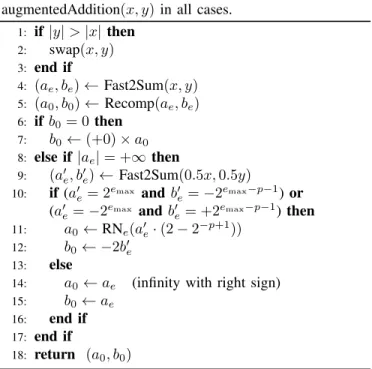
ALGORITHM 7: AA-Full(𝑥, 𝑦): computes augmentedAddition(𝑥, 𝑦) in all cases.
1: if |𝑦| > |𝑥| then 2: swap(𝑥, 𝑦) 3: end if 4: (𝑎𝑒, 𝑏𝑒) ← Fast2Sum(𝑥, 𝑦) 5: (𝑎0, 𝑏0) ← Recomp(𝑎𝑒, 𝑏𝑒) 6: if 𝑏0= 0 then 7: 𝑏0← (+0) × 𝑎0 8: else if |𝑎𝑒| = +∞ then 9: (𝑎′𝑒, 𝑏′𝑒) ← Fast2Sum(0.5𝑥, 0.5𝑦)
10: if (𝑎′𝑒= 2𝑒max and 𝑏′𝑒= −2𝑒max−𝑝−1) or
(𝑎′𝑒= −2𝑒max and 𝑏′
𝑒= +2𝑒max−𝑝−1) then
11: 𝑎0← RN𝑒(𝑎′𝑒· (2 − 2−𝑝+1))
12: 𝑏0← −2𝑏′𝑒
13: else
14: 𝑎0← 𝑎𝑒 (infinity with right sign)
15: 𝑏0← 𝑎𝑒
16: end if
17: end if
18: return (𝑎0, 𝑏0)
Theorem 2. The output (𝑎0, 𝑏0) of Algorithm 7 is equal to
augmentedAddition(𝑥, 𝑦). Proof.
1) if |𝑥 + 𝑦| < Ω + 2𝑒max−𝑝 then Item 1 of Theorem 1
tells us that the values 𝑎0 and 𝑏0 computed at Line 5 of
Algorithm 7 are equal to augmentedAddition(𝑥, 𝑦), with the possible exception that if 𝑏0= 0 it may have a sign
Standard. This possible error in the sign of 𝑏0is corrected at Lines 6-7. 2) if |𝑥 + 𝑦| = Ω + 2𝑒max−𝑝 then |𝑎 𝑒| = +∞. In that case, since 12· |𝑥 + 𝑦| = Ω 2 + 2
𝑒max−𝑝−1= 2𝑒max− 2𝑒max−𝑝−1,
at Line 9 we obtain
𝑎′= sign(𝑥 + 𝑦) · 2𝑒max
and
𝑏′= −sign(𝑥 + 𝑦) · 2𝑒max−𝑝−1.
In that case, Lines 10-12 of the algorithm return the correct values 𝑎0= sign(𝑥 + 𝑦) · Ω and 𝑏0= sign(𝑥 + 𝑦) · 2𝑒max−𝑝−1. 3) if |𝑥 + 𝑦| > Ω + 2𝑒max−𝑝 then |𝑎 𝑒| = +∞, and the
sum (𝑥 + 𝑦)/2 computed using Fast2Sum at Line 9 (without overflow since |𝑥 + 𝑦|/2 is less than or equal to the maximum of |𝑥| and |𝑦|) will be or absolute value (strictly) larger than 2𝑒max− 2𝑒max−𝑝−1, hence Lines
14-15 of the algorithm will be executed, and we will obtain 𝑎0= 𝑏0= sign(𝑥 + 𝑦) · ∞, as expected.
IV. USE OFALGORITHMRECOMP FOR IMPLEMENTING
AUGMENTEDMULTIPLICATION
A. General case
From two input floating-point numbers 𝑥 and 𝑦, we wish to compute RN0(𝑥 · 𝑦) and 𝑥 · 𝑦 − RN0(𝑥 · 𝑦) (or, merely,
RN0[︀𝑥 · 𝑦 − RN0(𝑥 · 𝑦)
]︀
when 𝑥 · 𝑦 − RN0(𝑥 · 𝑦) is not
a floating-point number). As we did for augmentedAddition, let us first present a simple algorithm (Algorithm 8 below). Unfortunately, it will be less general than the simple addition algorithm: this is due to the fact that when the absolute value of the product of two floating-point numbers is less than or equal to 2𝑒min+𝑝, it may not be exactly representable
by the sum of two floating-point numbers (an example is 𝑥 = 1 + 2−𝑝+1 and 𝑦 = 2𝑒min + 2𝑒min−𝑝+1: their product
2𝑒min + 2𝑒min−𝑝+2 + 2𝑒min−2𝑝+2 cannot be a sum of two
FP numbers, since such a sum is necessarily a multiple of 2𝑒min−𝑝+1).
ALGORITHM 8: AM-Simple(𝑥, 𝑦): computes augmentedMultiplication(𝑥, 𝑦) when
2𝑒min+𝑝+ 2𝑒min < |𝑥 · 𝑦| < Ω + 2𝑒max−𝑝.
1: (𝑎𝑒, 𝑏𝑒) ← Fast2Mult(𝑥, 𝑦)
2: (𝑎0, 𝑏0) ← Recomp(𝑎𝑒, 𝑏𝑒)
3: return (𝑎0, 𝑏0)
Theorem 3. The values 𝑎0 and 𝑏0 returned by Algorithm 8
satisfy:
1) If2𝑒min+𝑝+ 2𝑒min < |𝑥 · 𝑦| < Ω + 2𝑒max−𝑝(which implies
2𝑒min+𝑝+ 2𝑒min+1 ≤ |RN
𝑒(𝑥 · 𝑦)| ≤ Ω) then (𝑎0, 𝑏0) is
equal to augmentedMultiplication(𝑥, 𝑦), with the possible
exception that if𝑏0 = 0 it may have a sign that differs
from the one specified in the IEEE 754-2019 Standard; 2) if |𝑥 · 𝑦| = Ω + 2𝑒max−𝑝 = (2 − 2−𝑝) · 2𝑒max, then
𝑎0 = ±∞ (with the sign of 𝑥 · 𝑦) and 𝑏0 = ±∞ (with
the opposite sign) whereas the correct values would have been 𝑎0= ±Ω and 𝑏0 = ±2𝑒max−𝑝 (both with the sign
of𝑥 · 𝑦);
3) if |𝑥 · 𝑦| > Ω + 2𝑒max−𝑝, then 𝑎
0 = ±∞ (with the sign
of𝑥 · 𝑦) and 𝑏0= ±∞ (with the opposite sign) whereas
the correct values would have been𝑎0= 𝑏0= ±∞ (with
the sign of𝑥 · 𝑦).
Proof. The first item in Theorem 3 is a consequence of Lemma 2 and Lemma 8. If
2𝑒min+𝑝+ 2𝑒min< |𝑥 · 𝑦| < Ω + 2𝑒max−𝑝
then 2𝑒min+𝑝+ 2𝑒min+1≤ |RN
𝑒(𝑥 · 𝑦)| ≤ Ω, therefore ∙ (𝑎𝑒, 𝑏𝑒) = Fast2Mult(𝑥, 𝑦) gives 𝑎𝑒+ 𝑏𝑒= 𝑥 · 𝑦; ∙ |𝑎𝑒| > 2𝑒min ;
therefore Recomp(𝑎𝑒, 𝑏𝑒) returns the expected result.
The second item in Theorem 3 follows immediately by applying Algorithm 8 to the corresponding input value. Con-cerning the third item in Theorem 3, Table IV gives the values returned by Algorithm 8 when |𝑥 · 𝑦| > Ω + 2𝑒max−𝑝.
TABLE IV: Values obtained using Algorithm 8 when |𝑥 · 𝑦| > 2𝑒max(2 − 2−𝑝).
Algorithm 8 Result required
by the standard
𝑎0 +∞ · sign(𝑥 · 𝑦) +∞ · sign(𝑥 · 𝑦)
𝑏0 −∞ · sign(𝑥 · 𝑦) +∞ · sign(𝑥 · 𝑦)
As with the addition algorithm, if the signs of the zero variables matter in the target application and if Condition 1 of Theorem 3 is satisfied, it suffices to add the following lines to Algorithm 8 after Line 2:
if 𝑏0= 0 then
𝑏0← (+0) × 𝑎0
end if
(and, again, function copySign can be used if it is faster than a floating-point multiplication). Another solution is to notice that in Case 1 of Theorem 3, 𝑥𝑦−𝑎0is a floating-point number,
therefore one can just compute 𝑎0with Algorithm 8 and obtain
𝑏0 with one FMA instruction, as RN𝑒(𝑥𝑦 − 𝑎0). As we are
going to see that solution is useful even when Condition 1 of Theorem 3 is not satisfied.
Let us now build another augmented multiplication al-gorithm, Algorithm 9 below, that returns a correct re-sult even if the condition of Case 1 of Theorem 3 (i.e., 2𝑒min+𝑝+ 2𝑒min < |𝑥 · 𝑦| < Ω + 2𝑒max−𝑝) is not satisfied. We
need to be able to address the cases RN𝑒(𝑥 · 𝑦) = ±∞
(that correspond to items 2 and 3 in Theorem 3) and |RN𝑒(𝑥 · 𝑦)| ≤ 2𝑒min+𝑝.
This will be done by scaling the calculation, i.e., by finding a suitable power of 2, say 2𝑘, such that 2𝑘𝑥 is computed without
over/underflow, and the requested calculations (in particular those in Algorithm 8) can be done safely with inputs 𝑥′= 2𝑘𝑥
and 𝑦. We need to consider three cases:
∙ when RN𝑒(𝑥 · 𝑦) = ±∞, we choose 2𝑘= 1/2. This case
is dealt with in Section IV-B;
∙ when |RN𝑒(𝑥 · 𝑦)| ≤ 2𝑒min+1 − 2𝑒min−𝑝+1, we choose
2𝑘= 22𝑝. This case is dealt with in Section IV-C; ∙ when 2𝑒min+1≤ |RN
𝑒(𝑥 · 𝑦)| ≤ 2𝑒min+𝑝, we choose 2𝑘=
2𝑝. This case is dealt with in Section IV-D.
Note that when |RN𝑒(𝑥 · 𝑦)| ≤ 2𝑒min+𝑝 (i.e., in the last two
cases mentioned just above), RN0(𝑥𝑦 − RN0(𝑥𝑦)) = 0 does
not mean that 𝑥𝑦 − RN0(𝑥𝑦) = 0. This slightly complicates
the choice of the sign of 𝑏0 when it is equal to zero. More
precisely, when 𝑏0= 0, the sign of 𝑏0 must be:
∙ the sign of 𝑎0(i.e., the sign of 𝑥𝑦) when 𝑥𝑦 − 𝑎0= 0; ∙ the real sign of 𝑥𝑦 − 𝑎0 otherwise.
Fortunately, in both cases, this is the same sign as the one of RN𝑒(𝑥𝑦 − 𝑎0), which is obtained using an FMA instruction.
Hence, when 𝑏0 = 0, one can return (+0) · RN𝑒(𝑥𝑦 − 𝑎0)
(the multiplication by (+0) is necessary to handle the case 𝑥𝑦 − 𝑎0= 2𝑒min−𝑝, for which functions RN0 and RN𝑒differ).
B. First special case: if RN𝑒(𝑥 · 𝑦) = ±∞
In this case, which corresponds to Lines 2–11 in Al-gorithm 9, we need to know if we are in Case 2 (i.e., |𝑥 · 𝑦| = Ω + 2𝑒max−𝑝) or Case 3 (i.e., |𝑥 · 𝑦| > Ω + 2𝑒max−𝑝)
of Theorem 3. Hence our problem reduces to checking if |𝑥 · 𝑦| = Ω + 2𝑒max−𝑝. That problem is addressed easily. It
suffices to compute (𝑎′𝑒, 𝑏′𝑒) = Fast2Mult(0.5 · 𝑥, 𝑦):
∙ If |𝑥 · 𝑦| = Ω + 2𝑒max−𝑝, then (𝑥/2) · 𝑦 is computed by
Fast2Mult without overflow, which allows one to check its equality with ± (Ω + 2𝑒max−𝑝) /2;
∙ If it turns out that |𝑥 · 𝑦/2| ̸= (Ω + 2𝑒max−𝑝) /2 it suffices
to return 𝑎0 = 𝑏0 = RN𝑒(𝑥 · 𝑦): they will be infinities
with the right sign.
C. Second special case: if|RN𝑒(𝑥 · 𝑦)| ≤ 2𝑒min+1−2𝑒min−𝑝+1
In that case,
|𝑥 · 𝑦 − RN0(𝑥 · 𝑦)| ≤ 2𝑒min−𝑝, (5)
and thus RN0(𝑥 · 𝑦 − RN0(𝑥 · 𝑦)) = 0, so we have to return
𝑏0= 0 (with the sign of RN𝑒(𝑥𝑦 − 𝑎0)), and we only have to
focus on the computation of 𝑎0= RN0(𝑥 · 𝑦). We also assume
that RN𝑒(𝑥 · 𝑦) ̸= 0 (otherwise, it suffices to return the pair
(0, 0), with the sign of 𝑥𝑦). We therefore have
2𝑒min−𝑝 < |𝑥 · 𝑦| < 2𝑒min+1− 2𝑒min−𝑝. (6)
Note that (6) implies
2𝑒min+𝑝< |22𝑝𝑥 · 𝑦| < 2𝑒min+2𝑝+1− 2𝑒min+𝑝. (7)
Let us first give the general reasoning behind the calcu-lations of Lines 16–25 of Algorithm 9 (detailed proof will follow). Let 𝑎𝑒 be RN𝑒(𝑥 · 𝑦). Since the distance between
consecutive floating-point numbers in the vicinity of 𝑥𝑦 is
2𝑒min−𝑝+1 (we are in the subnormal range), we have the
following property:
∙ if 𝑥𝑦 = 𝑎𝑒− sign(𝑎𝑒) · 2𝑒min−𝑝 (i.e., we are in what we
call “Halfway case 1” in Section II), then 𝑎0= 𝑎𝑒− sign(𝑎𝑒) · 2𝑒min−𝑝+1; ∙ otherwise, 𝑎0= 𝑎𝑒.
Therefore, we need to compare 𝑥𝑦 with 𝑎𝑒−sign(𝑎𝑒)·2𝑒min−𝑝.
This cannot be done straightforwardly, because 𝑥𝑦 is not nec-essarily representable exactly as the sum of two FP numbers (Lemma 2 does not hold). Instead, we will compare 22𝑝𝑥𝑦
with 22𝑝𝑎
𝑒− sign(𝑎𝑒) · 2𝑒min+𝑝. The first step for doing that
will be to express 22𝑝𝑥𝑦 as the sum of two FP numbers 𝑡1
and 𝑡2 using Algorithm Fast2Mult. Then, to compare 𝑡1+ 𝑡2
with 22𝑝𝑎𝑒− sign(𝑎𝑒) · 2𝑒min+𝑝, we will first show that the
subtraction 𝑡3 = 𝑡1− 22𝑝𝑎𝑒 is performed exactly, so that it
will suffice to compare 𝑡2+ 𝑡3 with −sign(𝑎𝑒) · 2𝑒min+𝑝.
So, we successively compute (using FMA instructions) 𝑡1 = RN𝑒(︀(22𝑝· 𝑥) · 𝑦
)︀
𝑡2 = RN𝑒(︀(22𝑝· 𝑥) · 𝑦 − 𝑡1)︀ = 𝑥 · 𝑦 · 22𝑝− 𝑡1
𝑡3 = RN𝑒(︀𝑡1− 𝑎𝑒· 22𝑝)︀ .
First, 𝑡1 can be computed without overflow:
∙ |𝑥 · 𝑦| < 2𝑒min+1 and, since 𝑥 · 𝑦 ̸= 0, |𝑦| ≥ 2𝑒min−𝑝+1.
Therefore, |𝑥| ≤ 2𝑒min+1/2𝑒min−𝑝+1= 2𝑝, therefore
|𝑥| · 22𝑝< 23𝑝. Using (4), this implies that
|𝑥 · 22𝑝| < 2𝑒max+1, hence 𝑥 · 22𝑝 is a floating-point
number;
∙ now, |(22𝑝· 𝑥) · 𝑦| < 2𝑒min+1+2𝑝 < 23𝑝< 2𝑒max+1 since
𝑒min< 0.
Therefore, |22𝑝· 𝑥 · 𝑦| is below the overflow threshold, and
⃒ ⃒𝑡1− 22𝑝𝑥𝑦 ⃒ ⃒≤ 1 2ulp(𝑡1). (8) The fact that 𝑡2= 𝑥 · 𝑦 · 22𝑝− 𝑡1comes from Lemma 2 and
(7).
Let us show that 𝜃3= 𝑡1−𝑎𝑒·22𝑝is a floating-point number.
This will imply
𝑡3= 𝜃3= 𝑡1− 𝑎𝑒· 22𝑝
(hence, 𝜃3 can be computed with an FMA, or with an exact
multiplication by 22𝑝 followed by a subtraction). From (7) we obtain
2𝑒min+𝑝 ≤ |𝑡
1| ≤ 2𝑒min+2𝑝+1− 2𝑒min+𝑝+1
and ulp(𝑡1) ≤ 2𝑒min+𝑝+1.
Since 𝑎𝑒 (as any FP number) is a multiple of 2𝑒min−𝑝+1,
the number 22𝑝· 𝑎
𝑒 is a multiple of 2𝑒min+𝑝+1. Therefore, 𝜃3
is a multiple of ulp(𝑡1).
Now, (5) gives 𝑥 · 𝑦 − 2𝑒min−𝑝≤ 𝑎
𝑒≤ 𝑥 · 𝑦 + 2𝑒min−𝑝, from
which we deduce
𝑥 · 𝑦 · 22𝑝− 2𝑒min+𝑝 ≤ 𝑎
𝑒· 22𝑝≤ 𝑥 · 𝑦 · 22𝑝+ 2𝑒min+𝑝,
which implies, using (8), 𝑡1− 1 2ulp(𝑡1) − 2 𝑒min+𝑝≤ 𝑎 𝑒· 22𝑝≤ 𝑡1+ 1 2ulp(𝑡1) + 2 𝑒min+𝑝,
ALGORITHM 9: AM-Full(𝑥, 𝑦): computes augmentedMultiplication(𝑥, 𝑦) in all cases.
1: 𝑎𝑒← RN𝑒(𝑥 · 𝑦)
2: if |𝑎𝑒| = +∞ then
3: 𝑥′ ← 0.5 · 𝑥
4: (𝑎′𝑒, 𝑏′𝑒) ← Fast2Mult (𝑥′, 𝑦)
5: if (𝑎′𝑒= 2𝑒max and 𝑏′𝑒= −2𝑒max−𝑝+1) or
(𝑎′𝑒= −2𝑒max and 𝑏′
𝑒= +2𝑒max−𝑝+1) then
6: 𝑎0← RN𝑒(𝑎′𝑒· (2 − 2−𝑝+1))
7: 𝑏0← −2𝑏′𝑒
8: else
9: 𝑎0← 𝑎𝑒 (infinity with right sign)
10: 𝑏0← 𝑎𝑒
11: end if
12: else if |𝑎𝑒| ≤ 2𝑒min+𝑝 then
13: if 𝑎𝑒= 0 then
14: 𝑎0← 𝑎𝑒
15: 𝑏0← 𝑎𝑒
16: else if |𝑎𝑒| ≤ 2𝑒min+1− 2𝑒min−𝑝+1then
17: 𝑏0← 0
18: (𝑡1, 𝑡2) ← Fast2Mult (︀(𝑥 · 22𝑝), 𝑦)︀
19: 𝑡3← RN𝑒(𝑡1− 𝑎𝑒· 22𝑝)
20: 𝑧 ← RN𝑒(𝑡2+ 𝑡3)
21: if (𝑧 = −sign(𝑎𝑒) · 2𝑒min+𝑝) and
(RN𝑒(𝑧 − 𝑡3) = 𝑡2) then 22: 𝑎0← 𝑎𝑒− sign(𝑎𝑒) · 2𝑒min−𝑝+1 23: else 24: 𝑎0← 𝑎𝑒 25: end if 26: else 27: (𝑎′, 𝑏′) ← AM-Simple(2𝑝𝑥, 𝑦) 28: 𝑎0← RN𝑒(2−𝑝· 𝑎′) 29: 𝛽 ← RN𝑒(2−𝑝· 𝑏′)
30: if RN𝑒(2𝑝𝛽 − 𝑏′) = sign(𝛽) · 2𝑒min then
31: 𝑏0← 𝛽 − sign(𝛽) · 2𝑒min−𝑝+1 32: else 33: 𝑏0← 𝛽 34: end if 35: end if 36: else 37: 𝑏𝑒← RN𝑒(𝑥 · 𝑦 − 𝑎𝑒) 38: (𝑎0, 𝑏0) ← Recomp(𝑎𝑒, 𝑏𝑒) 39: end if 40: if 𝑏0= 0 then 41: 𝑏0← (+0) · RN𝑒(𝑥𝑦 − 𝑎0) 42: end if 43: return (𝑎0, 𝑏0) so that ⃒ ⃒𝑡1− 𝑎𝑒· 22𝑝 ⃒ ⃒≤ 1 2ulp(𝑡1) + 2 𝑒min+𝑝≤1 2ulp(𝑡1) + |𝑡1|. Hence, 𝜃3is a multiple of ulp(𝑡1) of magnitude less than or
equal to 12ulp(𝑡1) + |𝑡1|. Since 𝑡1 is a multiple of ulp(𝑡1), we
deduce that 𝜃3is a multiple of ulp(𝑡1) of magnitude less than
or equal to |𝑡1|. An immediate consequence (using Lemma 5)
is that 𝜃3 is a floating-point number, which implies 𝑡3= 𝜃3.
Now, we can compute 𝑎0= RN0(𝑥 · 𝑦). If
𝑥 · 𝑦 = 𝑎𝑒− sign(𝑎𝑒) · 2𝑒min−𝑝
then 𝑎0 = 𝑎𝑒 − sign(𝑎𝑒) · 2𝑒min−𝑝+1 (computed without
error), otherwise 𝑎0= 𝑎𝑒. Hence we have to decide whether
𝑥 · 𝑦 = 𝑎𝑒− sign(𝑎𝑒) · 2𝑒min−𝑝. This is equivalent to checking
if 𝑡2 + 𝑡3 = −sign(𝑎𝑒) · 2𝑒min+𝑝. This can be done as
follows: first note that since 𝑡3 is a multiple of ulp(𝑡1) and
|𝑡2| ≤ 12ulp(𝑡1), either 𝑡3 = 0 or |𝑡3| > |𝑡2|. Therefore,
Lemma 1 can be applied to the addition of 𝑡2 and 𝑡3. Item
2 of that lemma tells us that if we define 𝑧 = RN𝑒(𝑡2+ 𝑡3),
then RN𝑒(𝑧 − 𝑡3) = 𝑧 − 𝑡3. Therefore, checking if
𝑡2+ 𝑡3= −sign(𝑎𝑒) · 2𝑒min+𝑝
is equivalent to checking if
𝑧 = −sign(𝑎𝑒) · 2𝑒min+𝑝
and RN𝑒(𝑧 − 𝑡3) = 𝑡2.
D. Last special case: if2𝑒min+1≤ |RN
𝑒(𝑥 · 𝑦)| ≤ 2𝑒min+𝑝
That case corresponds to Lines 26–34 of Algorithm 9. In that case, we know that 𝑥 · 𝑦 − RN0(𝑥 · 𝑦) is of magnitude less
than or equal to 2𝑒min, but is not necessarily a floating-point
number. The standard requires that we return 𝑎0= RN0(𝑥 · 𝑦)
and 𝑏0= RN0(𝑥 · 𝑦 − RN0(𝑥 · 𝑦)).
We start by applying Algorithm 8 to the product (2𝑝𝑥) · 𝑦. That product can be computed without overflow:
∙ first, |RN𝑒(𝑥 · 𝑦)| ≤ 2𝑒min+𝑝 implies
|𝑥𝑦| ≤ 2𝑒min+𝑝+ 2𝑒min. Also, 2𝑒min+1 ≤ |RN 𝑒(𝑥 · 𝑦)| implies 𝑦 ̸= 0, therefore |𝑦| ≥ 2𝑒min−𝑝+1. Thus |𝑥| = ⃒ ⃒ ⃒ ⃒ 𝑥𝑦 𝑦 ⃒ ⃒ ⃒ ⃒ ≤2 𝑒min+𝑝+ 2𝑒min 2𝑒min−𝑝+1 = 2 2𝑝−1+ 2𝑝−1.
Therefore |2𝑝𝑥| ≤ 23𝑝−1+22𝑝−1< 2𝑒maxusing (4). Thus
(2𝑝𝑥) is below the overflow threshold. ∙ finally, |𝑥𝑦| ≤ 2𝑒min+𝑝+ 2𝑒min implies
|(2𝑝𝑥) · 𝑦| ≤ 2𝑒min+2𝑝+ 2𝑒min+𝑝,
which is less than 2𝑒max from (4) and the fact that 𝑒
min
is negative.
Algorithm 8 applied to (2𝑝𝑥) · 𝑦 returns two values, say 𝑎′ and 𝑏′, such that 𝑎′ = RN0(2𝑝𝑥 · 𝑦) and 𝑏′= 2𝑝𝑥 · 𝑦 − 𝑎′. We
immediately deduce using Lemma 6 that 2−𝑝𝑎′is the expected RN0(𝑥 · 𝑦). Obtaining RN0(𝑥 · 𝑦 − 2−𝑝𝑎′) = RN0(2−𝑝𝑏′)
is slightly more tricky (Lemma 6 cannot be used because |2−𝑝𝑏′| can be strictly less than 2𝑒min). We first compute
𝛽 = RN𝑒(2−𝑝𝑏′). The number 𝛽 is equal to the expected
RN0(2−𝑝𝑏′) unless we are in Halfway Case 1 of Section II,
i.e., unless
𝛽 − (2−𝑝𝑏′) = sign(𝛽) · 2𝑒min−𝑝 (9)
in which case, one should replace 𝛽 by 𝛽 −sign(𝛽)·2𝑒min−𝑝+1.
Equation (9) is equivalent to
a condition which is easy to test since the subtraction is exact: 2𝑝𝛽 − 𝑏′ is a multiple of 2𝑒min−𝑝+1, of magnitude less than or
equal to 2𝑒min, hence it is a floating-point number.
All this gives Algorithm 9 and Theorem 4.
Theorem 4. The output (𝑎0, 𝑏0) of Algorithm 9 is equal to
augmentedMultiplication(𝑥, 𝑦).
V. FORMAL PROOF
Arithmetic algorithms can be used in critical applications. The proof presented here is complex, with many particular cases to be considered. We have used the Coq proof assis-tant and the Flocq library [2] for our development towards Theorems 1 and 4.
Our formal proof is available as electronic appendix. Note that we have aimed at genericity. In particular, we have tried to generalize the tie-breaking rule when possible. The precision and minimal exponent are hardly constrained as we only require 𝑝 > 1 and 𝑒min < 0. As explained above,
the radix must be 2 as Algorithm 4 does not hold for radix 10 (the definitions and first properties of ulp𝐻 and RN0 are
generic though).
The formal proof quite follows the mathematical proof described above. Of course, we had to add several lemmas and to define RN0 and its properties. This definition was
very similar to the definition of rounding-to-nearest with tie-breaking away from zero defined by the standard for decimal arithmetic [8], and most of the proofs were nearly identical.
We then proved the correctness of Algorithm 4. In this case for |𝑎| > 2𝑒min, the two RN
𝑒roundings may be replaced with a
rounding to nearest with any tie-breaking rule (they may even differ). Algorithm 5 is also proven. Similarly, the two RN𝑒
roundings may in fact use any tie-breaking rule. The proof of Theorem 1 is then easily deduced, with Recomp using any two tie-breaking rules.
As on paper, the proof of Theorem 4 is more intricate, with many subcases, even if we handle only cases A (without the zeroes), C, and D. Here, the case split depends on the tie-breaking rule: the equalities may be either strict or large de-pending upon the tie-breaking rule. For the sake of simplicity, we chose to stick to the pen-and-paper proof and share the same case split. We then require some roundings to use tie-breaking to even. We were not able to generalize the proof at a reasonable cost to handle all tie-breaking rules. Nevertheless, the proof was formally done and we were able to prove the correctness of Theorems 1 and 4 (without considering overflows and signs of zeroes). The Coq statements are as follows (with few simplifications for the sake of readability). Note that c1. . . c7 are arbitrary tie-breaking rules.
DefinitionRecomp:=func1 c2 a b⇒
letz:= round_flt c1 (psi*a)in
letd:= round_flt c2 (z−a)in
if(Req_bool (2*b) d)then(z,−b)else(a,b).
DefinitionAA_Simple:=func1 c2 x y⇒
let(x’,y’) := if(Rlt_bool (Rabs x) (Rabs y))
then(y,x)else(x,y)in
let(ae,be) := Fast2Sum x’ y’in
Recomp c1 c2 ae be.
DefinitionAM_Full:=func1 c2 c3 c4 c5 c6 c7 x y⇒
letae:= round_flt ZnearestE (x*y)in
if(Rle_bool (Rabs ae) (bpow (emin+prec)))then
(* zero *)
if(Req_bool ae 0)then(0,0)else
(* very small *)
if(Rle_bool (Rabs ae) (bpow (emin+1) −
bpow(emin−prec+1)))then
lett1:= round_flt c1 (x*(y*bpow (2*prec)))in
lett2:= round_flt c2 (x*(y*bpow (2*prec)) − t1)in
lett3:= round_flt c3 (t1 − ae*bpow (2*prec))in
letz:= round_flt ZnearestE (t2+t3)in
if(andb (Req_bool z (−sign(ae)*bpow (emin+prec)))
( Req_bool (round_flt ZnearestE (z−t3)) t2))
then(ae−sign(ae)*bpow (emin−prec+1),0)
else(ae,0)
(* medium small*)
else lett1:= round_flt c1 (x*(y*bpow prec))in
lett2:= round_flt c2 (x*(y*bpow prec) − t1)in
letA’ := Recomp emin prec c3 c4 t1 t2in
leta0:= round_flt c5 (bpow (−prec)*fst A’)in
letbeta:= round_flt c6 (bpow (−prec)*snd A’)in
letz:= round_flt c7 (bpow prec*beta−snd A’)in
if(Req_bool z (sign beta*bpow emin))
then(a0, beta − sign(beta)*bpow (emin−prec+1))
else(a0,beta)
(*big*)
else
letbe:= round_flt ZnearestE (x*y−ae)in
Recomp c1 c2 ae be.
LemmaAA_Simple_correct:forallc1 c2 x y,
format_flt x→ format_flt y →
let(a0,b0) := AA_Simple c1 c2 x yin
x+y = a0 + b0 ∧ a0 = round_flt Znearest0 (x+y).
LemmaAM_Full_correct:forallc1 c2 c3 c4 c5 c6 c7 x y,
format_flt x→ format_flt y →
let(a0,b0) := AM_Full c1 c2 c3 c4 c5 c6 c7 x yin
a0= round_flt Znearest0 (x*y)
∧ b0 = round_flt Znearest0 (x*y−a0).
A very important limitation of these proofs is that overflows, infinite numbers, and the signs of zeroes are not considered. We relied on the Flocq formalization that considers floating-point numbers as a subset of real numbers. Therefore, zeroes are merged and there are neither infinities, nor NaNs. It allows us to state the final theorems in the most understandable way: 𝑎0 = RN0(𝑡) and 𝑎0+ 𝑏0 = 𝑡 or at least 𝑏0 = RN0(𝑡 − 𝑎0)
(with 𝑡 being either the sum or product of two floating-point numbers).
We have tried to develop additional formal proofs taken all exceptional behaviors into account (especially NaNs and over-flows). We have relied on a modified version of the Binary definitions of Flocq and we have defined the full algorithms, with comparisons on FP numbers and possible overflows. It made both the algorithms and their specifications more complicated and less readable. Moreover, the comprehensive formal proofs were out of reach, both by lack of support lemmas and by combinatorial explosion of the subcases for each and every operation (NaN, overflow, signed zero, and so
on). This really calls for automations in Coq for handling FP numbers with exceptional behaviors, that is out of scope of this paper.
VI. IMPLEMENTATION AND COMPARISON
We have implemented the algorithms presented in this paper in binary64 (a.k.a. double precision) arithmetic, as well as emulation algorithms based on integer arithmetic, described below. We used an Intel Core i7-7500U x86_64 processor clocked at 2.7GHz under GNU/Linux (Debian 4.19.0-8-amd64), and the programs were compiled using GCC (Debian 8.3.0-6) 8.3.0, with the option -O3 -march=native. Our implementation, together with all testing and performance evaluation code, is available as additional material coming with this article; it can be downloaded at https://gitlab.com/cquirin/ ieee754-2019-augmented-operations-reference-implementation and is archived at https://hal.archives-ouvertes.fr/ hal-02137968.
Having an integer-based version of the augmented opera-tions was important for comparison purposes, since there are no other implementations of these operations at the time we are writing this paper. Importantly enough, as we are going to see below, the integer-based algorithms are not simpler than the floating-point based algorithms presented in this paper. This is because the floating-point operations somehow automatically handle most special cases.
The integer-based emulation code proceeds as follows (as-suming here we use the binary64 format):
1) The inputs 𝑥 and 𝑦 are checked for special values, such as NaN or infinities. For these special values, a regular FP addition or multiplication is executed, in order to get correct setting of flags and special values for the high order result 𝑎. For 𝑏, the same value is used. Similar logic is used for zero inputs.
2) Finite, non-zero, regular FP inputs 𝑥 and 𝑦 are decom-posed into (−1)𝑠𝑥2𝐸𝑥𝑀
𝑥 and (−1)𝑠𝑦2𝐸𝑦𝑀𝑦 where
𝑀𝑥 and 𝑀𝑦 are normalized integer significands stored
on 64-bit integer variables. This step includes a normal-ization step using the integer hardware lzc (leading-zero count) instruction whenever 𝑥 or 𝑦 are subnormal. The hidden bit is made explicit.
3) For addition, the two couples (𝑠𝑥, 𝐸𝑥, 𝑀𝑥) and
(𝑠𝑦, 𝐸𝑦, 𝑀𝑦) are ordered for exponents: 𝐸𝑥≥ 𝐸𝑦. When
the exponent difference exceeds a certain limit, addition returns the ordered 𝑥 and 𝑦 as 𝑎 and 𝑏 as-is.
4) For all other cases, a temporary exact intermediate result (−1)𝑠2𝐸𝑀 is formed, where the integer significand 𝑀
is stored on a 128-bit variable, which the compiler em-ulates on two 64-bit registers and the appropriate use of addition-with-carry and high/low-part multiplication ma-chine instructions. For addition, this intermediate result is obtained by shifting the ordered 𝑀𝑥 integer significand
by 𝐸𝑥− 𝐸𝑦 places to the left and adding or subtracting
𝑀𝑦. For multiplication, it suffices to multiply 𝑀𝑥and 𝑀𝑦
with a 64-by-64-gives-128 bit multiplication. The integer significand 𝑀 is normalized (unless it becomes zero due
to cancellation), which requires a branch and a 1-bit shift for multiplication and a leading-zero count and a larger, 128-bit shift (across 64-bit registers) for addition. 5) The intermediate result (−1)𝑠2𝐸𝑀 is rounded to the
nearest IEEE754 binary64 value 𝑎, applying round-to-nearest-ties-to-zero rules. This rounding step is imple-mented as a “rounding to odd” [3] (with sticky bit) to (−1)𝑠2𝐸′𝑀′, where 𝑀′ is a 64-bit integer significand,
followed by the actual rounding to the binary64 format. This code sequence is quite complicated as it must cope with a multitude of possible cases, such as overflow, gradual or complete underflow as well as exact zeroes. A trace of overflow, underflow and inexact rounding is kept during this rounding step.
6) The high-order word 𝑎 is decomposed again into (−1)𝑠𝑎2𝐸𝑎𝑀
𝑎. If it is finite, this value is subtracted
from the intermediate result (−1)𝑠2𝐸𝑀 , which, after
appropriate leading-zero count and normalization shift, yields to (−1)𝑠ℓ2𝐸ℓ𝑀
ℓ, where 𝑀ℓ is an integer
signifi-cand stored on a 64-bit integer. This value (−1)𝑠ℓ2𝐸ℓ𝑀
ℓ
is given to the same rounding code as the one used above, which yields 𝑏 with round-to-nearest-ties-to-zero and a trace of overflow1, underflow and inexact rounding.
7) Out of both traces for overflow, underflow and inexact a global IEEE754 flag setting is computed and applied to IEEE754 flag registers by executing a dummy FP operation that make the appropriate flags be raised. The emulation code has the advantage of being the only version of our algorithms that is able to set the IEEE754 flags correctly and to be insensible to the prevailing IEEE754 rounding direction attribute. The FP-based algorithms may set the inexact flag as well as other flags spuriously. They do require the IEEE754 rounding direction attribute to be round-to-nearest-ties-to-even, which is the default. However, these advantages of the emulation code come at a significant cost: as we are going to see, the emulation code is on average 1.5 to 20 times slower than the FP-based algorithms. The emulation code also has the disadvantage of being rather complex. The precise rounding logic for round-to-nearest-ties-to-zero for example is quite complicated, which required extra care at its development to overcome its error-prone nature.
The statistical distribution of the number of cycles used by our algorithms (using 106 samples, with the distributions of the inputs described below) is given:
∙ for the augmentedAddition algorithms, in Figures 4a for Algorithm 6 (AA-Simple), 4b for Algorithm 7 (AA-Full), and 4c for the integer-based emulation of augmentedAd-dition;
∙ for the augmentedMultiplication algorithms, in Figures 5a for Algorithm 8 Simple), 5b for Algorithm 9 (AM-Full), and 5c for the integer-based emulation of augment-edMultiplication.
For each input sample, formed by an input couple (𝑥, 𝑦), the number of cycles is measured as follows: the function implementing one of our algorithms is run on 𝑥 and 𝑦. Its execution time is measured by reading off the x86 Time
0 5 10 15 20 25 0 20 40 60 80 100
(a) Algorithm 6 (all simple inputs)
0 5 10 15 20 25 30 0 20 40 60 80 100
(b) Algorithm 7 (all inputs)
0 5 10 15 20 25 30 0 20 40 60 80 100
(c) Emulation algorithm (all inputs)
Fig. 4: Statistical distribution of the number of cycles for the addition algorithms
Step Counter with the rdtsc instruction before and after the execution of the function. Before reading the Time Step Counter, the CPU’s pipeline is serialized by executing a dummy cpuid instruction, which Intel documents as having this serialization effect. As the time measurements obtained by subtracting the before Time Step Counter’s value from the after counter’s value also include the time for pipeline serialization, execution of the rdtsc instruction and the function call itself, the same measurement is repeated with an empty function that has the same signature as the actual function to time. The empty function’s measured execution time is subtracted off the actual function’s measured execution time. This yields a raw execution time sample in cycles. All raw execution times that are less than 1 cycle are discarded and the timing procedure is repeated. The measurement yielding to positive raw execution times is repeated 100 times, an average and maximum value is computed. If the average value does not differ from the maximum value by more than a certain amount (typically 25%), the average value is taken as the execution time in cyclesfor this input sample (𝑥, 𝑦). The measurements are taken on a CPU not executing any other heavy jobs, after a preheating phase for the instruction cache. The Linux scheduler is configured to keep the process on one CPU core as long as possible. Core migration is anyway filtered out by our testing strategy as it yields either negative raw timings or raw timings that are clear outliers. Overall, 106 different
samples are timed, which yields to the histograms illustrated in Figures 4 and 5 as well as the average values (averaging over all 106 inputs) reported in Tables V and VI.
The different input samples (𝑥, 𝑦) are produced as follows:
∙ The all cases input samples are produced with a
pseudo-random number generator such that all signs, exponents and significands are uniformly distributed among all binary64 FP values (𝑥, 𝑦) that are finite numbers such that the resulting outputs (𝑎, 𝑏) are finite as well. The filtering of whether or not a candidate (𝑥, 𝑦) produces finite outputs (𝑎, 𝑏) uses our integer-based emulation code to compute (𝑎, 𝑏) out of the candidate (𝑥, 𝑦).
∙ The all simple cases input samples are produced by filtering from the set of the all cases samples the ones for which the simple FP-based Algorithms 6 and 8 produce bit-correct results (including correct signs for zeroes). The decision of whether or not a candidate sample (𝑥, 𝑦) is
an all simple case is taken by comparing the output of the respective FP-based simple algorithm with the one of our integer-based emulation code.
∙ The halfway cases input samples (𝑥, 𝑦) are such that the respective outputs (𝑎, 𝑏) are finite FP numbers (zero and non-zero but no overflows) and 𝑥 + 𝑦 resp. 𝑥 × 𝑦 is precisely in the middle between two binary64 FP numbers. They are produced as follows:
– For addition in binary64, a 54 bit odd integer number 𝑁 is produced2 along with a uniformly distributed
exponent 𝐸. A uniformly distributed split-point 𝜎 ∈ {1, . . . , 53} is then produced. Using 𝜎, 𝑁 is cut into two parts which, along with 𝐸 and 𝜎, yield to the exponents and significands of candidates 𝑥 and 𝑦. Half of the values 𝑥 and 𝑦 are swapped. The “cutting” process is not actually just a bit cut but done in such a way that both 𝑥 and 𝑦 can be both negative or positive. – For multiplication on binary64, two uniformly dis-tributed 27 bit odd integers are produced along with uniformly distributed exponents.
The candidate (𝑥, 𝑦) samples are checked for finiteness and whether or not they produce finite outputs (𝑎, 𝑏); all candidates that do not satisfy these constraints are filtered out.
∙ The halfway simple cases are obtained by filtering from the halfway cases the ones for which the simple FP-based algorithms produce correct result, similarly as to how the all simple casesare obtained.
The average timings are given in the first half of Table V for the augmentedAddition algorithms, and the first half of Table VI for the augmentedMultiplication multiplication algo-rithms. In each of these tables, the second half gives average timings for halfway cases.
Concerning augmentedAddition, Algorithm 7 is slightly better than the integer-based emulation in the general case, and significantly better in the bad cases. Concerning augmented-Multiplication, Algorithm 9 is significantly better, except on very rare cases (at the extreme right of Figure 5b). In all cases, the “simple” versions of the algorithms (Algorithms 6 and 8) are significantly faster in the cases when they work. They may also be significantly slower when they do not work, due to
2This actually means that only 52 bits are random, as the 53rd bit and the
0 10 20 30 40 50 60 0 50 100 150 200 250 300
(a) Algorithm 8 (all simple inputs)
0 5 10 15 20 25 30 0 50 100 150 200 250 300
(b) Algorithm 9 (all inputs)
0 5 10 15 20 25 30 0 50 100 150 200 250 300
(c) Emulation algorithm (all inputs)
Fig. 5: Statistical distribution of the number of cycles for the multiplication algorithms
hardware constraints; for instance, Algorithm 8 may make the hardware produce and consume subnormal FP values, which is a slow process on some architectures.
TABLE V: Average timings in cycles for the augmentedAd-dition algorithms
Algorithm ♯ of cycles
Algorithm 6 (addition, all simple cases) 7.66
Algorithm 7 (addition, all cases) 10.46
Integer-based emulation of addition (all cases) 14.70
Algorithm 6 (addition, halfway simple cases) 7.74
Algorithm 7 (addition, halfway cases) 9.82
Integer-based emulation of addition (halfway cases) 4.99
TABLE VI: Average timings in cycles for the augmentedMul-tiplication algorithms
Algorithm ♯ of cycles
Algorithm 8 (multiplication, all simple cases) 7.62
Algorithm 9 (multiplication, all cases) 13.45
Integer-based emulation of multiplication (all cases) 75.65
Algorithm 8 (multiplication, halfway simple cases) 3.15
Algorithm 9 (multiplication, halfway cases) 4.99
Integer-based emulation of multiplication (halfway cases) 58.34
CONCLUSION
We have presented and implemented algorithms that allow one to emulate the newly suggested “augmented” floating-point operations using the classical, rounded-to-nearest ties-to-even, operations. The algorithms are very simple in the general case. Special cases are slightly more involved but will remain infrequent in most applications. These algorithms compare favorably with an integer-based emulation of the augmented operations. Furthermore, the availability of both tests for special cases and formal proofs covering normal and underflow cases (despite the limitations presented in Section V) gives much confidence in these algorithms.
ACKNOWLEDGEMENT
We thank Claude-Pierre Jeannerod for his very useful sug-gestions.
REFERENCES
[1] S. Boldo, S. Graillat, and J.-M. Muller. On the robustness of the 2Sum and Fast2Sum algorithms. ACM Transactions on Mathematical Software, 44(1):4:1–4:14, July 2017.
[2] S. Boldo and G. Melquiond. Computer Arithmetic and Formal Proofs. ISTE Press – Elsevier, 2017.
[3] Sylvie Boldo and Guillaume Melquiond. Emulation of FMA and
correctly rounded sums: proved algorithms using rounding to odd. IEEE Transactions on Computers, 57(4):462–471, April 2008.
[4] T. J. Dekker. A floating-point technique for extending the available precision. Numerische Mathematik, 18(3):224–242, 1971.
[5] J. Demmel, P. Ahrens, and H. D. Nguyen. Efficient reproducible floating point summation and BLAS. Technical Report UCB/EECS-2016-121, EECS Department, University of California, Berkeley, June 2016.
[6] J. Harrison. A machine-checked theory of floating point arithmetic.
In 12th International Conference in Theorem Proving in Higher Order Logics (TPHOLs), volume 1690 of Lecture Notes in Computer Science, pages 113–130. Springer-Verlag, Berlin, September 1999.
[7] J. R. Hauser. Handling floating-point exceptions in numeric programs. ACM Transactions on Programming Languages and Systems, 18(2):139– 174, 1996.
[8] IEEE. IEEE Standard for Floating-Point Arithmetic (IEEE Std 754-2019). July 2019.
[9] C.-P. Jeannerod, J.-M. Muller, and P. Zimmermann. On various ways to split a floating-point number. In 25th IEEE Symposium on Computer Arithmetic, Amherst, MA, USA, pages 53–60, June 2018.
[10] W. Kahan. Lecture notes on the status of IEEE-754. Available at http: //www.cs.berkeley.edu/~wkahan/ieee754status/IEEE754.PDF, 1997. [11] D. E. Knuth. The Art of Computer Programming, volume 2.
Addison-Wesley, Reading, MA, 3rd edition, 1998.
[12] O. Møller. Quasi double-precision in floating-point addition. BIT, 5:37– 50, 1965.
[13] J.-M. Muller, N. Brunie, F. de Dinechin, C.-P. Jeannerod, M. Joldes,
V. Lefèvre, G. Melquiond, N. Revol, and S. Torres. Handbook of
Floating-Point Arithmetic. Birkhäuser Boston, 2018.
[14] Y. Nievergelt. Scalar fused multiply-add instructions produce floating-point matrix arithmetic provably accurate to the penultimate digit. ACM Transactions on Mathematical Software, 29(1):27–48, 2003.
[15] E. J. Riedy and J. Demmel. Augmented arithmetic operations proposed for IEEE-754 2018. In 25th IEEE Symposium on Computer Arithmetic, Amherst, MA, USA, pages 45–52, June 2018.
[16] S. M. Rump. Ultimately fast accurate summation. SIAM Journal on Scientific Computing, 31(5):3466–3502, January 2009.
[17] P. H. Sterbenz. Floating-Point Computation. Prentice-Hall, Englewood Cliffs, NJ, 1974.