Learning and comparing functional connectomes across subjects

HAL Id: hal-00812911

https://hal.inria.fr/hal-00812911

Submitted on 13 Apr 2013

HAL is a multi-disciplinary open access

archive for the deposit and dissemination of

sci-entific research documents, whether they are

pub-lished or not. The documents may come from

teaching and research institutions in France or

abroad, or from public or private research centers.

L’archive ouverte pluridisciplinaire HAL, est

destinée au dépôt et à la diffusion de documents

scientifiques de niveau recherche, publiés ou non,

émanant des établissements d’enseignement et de

recherche français ou étrangers, des laboratoires

publics ou privés.

Learning and comparing functional connectomes across

subjects

Gaël Varoquaux, R. Cameron Craddock

To cite this version:

Gaël Varoquaux, R. Cameron Craddock. Learning and comparing functional connectomes across

sub-jects. NeuroImage, Elsevier, 2013, 80, pp.405-415. �10.1016/j.neuroimage.2013.04.007�. �hal-00812911�

Learning and comparing functional connectomes across subjects

Ga¨el Varoquauxa,b,c,∗_{, R. Cameron Craddock}d,e

a

Parietal project-team, INRIA Saclay-ˆıle de France b

INSERM, U992 c

CEA/Neurospin bˆat 145, 91191 Gif-Sur-Yvette d

Child Mind Institute, New York, New York e

Nathan Kline Institute for Psychiatric Research, Orangeburg, New York

Abstract

Functional connectomes capture brain interactions via synchronized fluctuations in the functional magnetic resonance imaging signal. If measured during rest, they map the intrinsic functional architecture of the brain. With task-driven experiments they represent integration mechanisms between specialized brain areas. Analyzing their variability across subjects and conditions can reveal markers of brain pathologies and mechanisms underlying cognition. Methods of estimating functional connectomes from the imaging signal have undergone rapid developments and the literature is full of diverse strategies for comparing them. This review aims to clarify links across functional-connectivity methods as well as to expose different steps to perform a group study of functional connectomes.

Keywords: Functional connectivity, connectome, group study, effective connectivity, fMRI, resting-state

1. Introduction

Functional connectivity reveals the synchronization of distant neural systems via correlations in

neurophysiolog-ical measures of brain activity [14, 37]. Given that

high-level function emerges from the interaction of specialized

units [110], functional connectivity is an essential part of

the description of brain function, that complements the localizationist picture emerging from the systematic

map-ping of regions recruited in tasks [101]. However, while

there exists a well-defined standard analysis framework for activation mapping that enables statistically-controlled

comparisons across subjects [39], group-level analysis of

functional connectivity still face many open methodolog-ical challenges. Deriving a picture of a single subject’s functional connectivity is by itself not straightforward, as the brain comprises a myriad of interacting subsystems and its connectivity must be decomposed into simplified and synthetic representations. An important view of brain connectivity is that of distributed functional networks

de-picted by their spatial maps [31]. Another no less

impor-tant and complementary view is that of connections

link-ing localized functional modules depicted as a graph [17].

This representation of brain connectivity is often called

the functional connectome [102] and is the focus of intense

worldwide research efforts as it holds promises of new

in-sights in cognition and pathologies [13,30,45].

The purpose of this paper is to review methodological progress in the estimation of functional connectomes from

∗_{Corresponding author}

blood oxygenation level dependent (BOLD) based func-tional magnetic resonance imaging (fMRI) data and their comparisons across individuals. It does not attempt to be exhaustive, as the field is wide and moving rapidly, but de-tails specific tools and guidelines that, in the experience of the authors, lead to controlled and powerful inter-subject comparisons. The paper is focused on functional connec-tomes in contrast to structural connecconnec-tomes, as the infer-ence of functional connectivity requires important statisti-cal modeling considerations that are vastly different from the complications involved with estimating structural con-nectivity. While the notion of functional connectomics is

often associated with the study of resting state [13], the

methods presented in this paper are also relevant for task-based studies. On the other hand, the paper has a focus on fMRI; although the core concepts presented can be applied to magnetoencephalography (MEG) or

electroencephalog-raphy (EEG) [103], additional specific problems such as

source reconstruction must be considered [93].

“Functional connectivity” is defined as a measure of

synchronization in brain signals [35]. More generally, it

is interesting as a window on underlying synchrony on

neural processes [63]. By “functional connectome”, here

we specifically denote a graph representing functional in-teractions in the brain, where the term “graph” is taken in its mathematical sense: a set of nodes connected to-gether by edges. Graph nodes (brain regions) correspond to spatially-contiguous and functionally-coherent patches of gray matter and edges describe long-range synchroniza-tions between nodes that are putatively subtended by large

fiber pathways [68]. A graph can be weighted or not,

symmetric matrix tabulating the connection weights be-tween each pair of nodes. Functional-connectivity graphs are used to represent evoked activity, as in task-response

studies [72], as well as ongoing activity, present in the

ab-sence of specific tasks or in the background during task and often studied in so-called resting state experiments

[83]. Another important notion that arises from the study

of distributed modes of brain function is that of specialized

functional networks1_{[31]. With our definition of the}

func-tional connectome, funcfunc-tional networks are not directly building blocks of the connectome but appear as a

conse-quence of the graphical structure [116,117].

The paper is organized as follows. First we discuss es-timation of functional connectomes. This part, akin to a first-level analysis in standard activation mapping method-ology, is not in itself a group-level operation, but it is a critical step for inter-subject comparison. In a following section, we discuss several strategies for comparing con-nectomes across subjects. Finally we discuss the links be-tween the representation of brain connectivity as graphs of functional connectivity and more complex models, such as effective-connectivity models.

2. Estimating functional connectomes

Here we discuss the inference of connectomes from functional brain imaging data. We start with preprocess-ing considerations, followed by the choice of nodes i.e. re-gions, signal extraction, and the estimation of graphs. 2.1. Preprocessing considerations

In addition to standard preprocessing performed for task-based analysis (slice-timing correction, realign-ment, spatial normalization, and possibly smoothing), connectivity-based analysis require additional denoising to separate intrinsic activity from confounding signals. This process involves regressing time series capturing sources of structured noise from the fMRI data. Physiological noise due to cardiac and respiration are two important

noise signals [11, 12, 53, 67] that are difficult to control

for and as a result are not commonly regressed out. In-stead the mean signal from white matter (WM) and cere-brospinal fluid (CSF) are used as surrogates to measure these sources of noise as well as other scanner induced

sig-nal fluctuations [31,67]. More complex models account for

spatial variation in noise by incorporating voxel-specific

re-gressors of neighboring WM (ANATICOR [55]) or the top

components from a principal components analysis of

high-variance signals (CompCor [7]). Head motion induced

sig-nal fluctuations are accounted for by incorporating

move-ment parameters [31,41,67]. The global mean time series

1

In neuroimaging, the term network is sometimes used to denote a graph of brain function. To disambiguate the notion of segregated spatial mode [31] from that of connectivity graphs, we will purposely restrict its usage in this paper.

has been proposed as an additional noise regressor that appears to improve the spatial specificity of connectivity

results [31, 32]. This practice has become controversial

since the global signal regression introduces negative

corre-lations [19,77,90]. Removing these sources of nuisance in

addition to linear trends results in more contrasted corre-lation matrices that improve the delineation of functional

structures (fig.2).

Filtering to remove high frequencies is often performed, based on the initial observation that fluctuations impli-cated in resting-state functional connectivity are

predom-inately slower than 0.1 Hz [14, 23]. While high-pass and

low-pass filtering decrease the impact of some confounds, recent studies have shown that connectivity is present

across the full spectrum of observed frequencies [99,113].

Regressing out a good choice of confound signals is more specific than frequency filtering, and in our experience

gives more contrasted correlation matrices2_{. In addition,}

the recent developments of very rapid acquisition proto-cols prevent aliasing of the physiological noise with the neural signal and give access to more specific noise

con-founds than traditional low-TR sequences [16].

It is important to keep in mind that the proposed cor-rection strategies are approximate and not definitive tech-niques. This has become particularly apparent for head motion with reports that micromovements on the scale of

≤0.2 mm can induce artefactual group-level findings even

when motion is accounted for in preprocessing [82,92,112].

Special care must be taken to adequately control for

resid-ual impact of head motion in the group model [92,112].

2.2. Defining regions

The choice of regions of interests (ROIs) that define the nodes of the graphs can be very important both in the estimation of connectomes and for group comparison

[119]. Unsurprisingly, simulations have shown that

ex-tracting signal from ROIs that did not match functional

units would lead to erronous graph estimation [100].

Dif-ferent strategies to define suitable ROIs coexist. While dense parcellation approaches cover a large fraction of the

brain [1,8,25,116,119], this coverage can be traded off to

focus on some specific regions, in favor of increased func-tional specificity and thus better differentiation across

net-works [28,46,114]. In addition, while ROIs are most often

defined as a hard selection of voxels, it is also possible to use a soft definition, attributing weights as with proba-bilistic atlases, or spatial maps of functional networks ex-tracted from techniques such as independent component

analysis (ICA) [57,99].

Regions from atlases. Atlases can be used to define full-brain parcellations. Popular choices are the Automatic

Anatomic Labeling (AAL) atlas [111], which benefits from

2

Note that naive use of filtering can induce spurious correlations [26].

an SPM toolbox, or the ubiquitous Talaraich-Tournoux

at-las [107]. However, these atlases suffer from major

short-comings; namely i) they were defined on a single subject and thus do not reflect inter-subject variability, and ii) they focus on labeling large anatomical structures and do not match functional layout –for instance only two re-gions describe the medial part of the frontal lobe in the

AAL atlas. Multi-subject probabilistic altases such as

the Harvard-Oxford atlas distributed with FSL [98] or the

sulci-based structural atlas used in [116] mitigate the first

problem, and the high number of regions defined using sulci also somewhat circumvent the second problem (see

fig.1).

Defining regions from the literature. Regions can be de-fined from previous studies, informally or with system-atic meta-analysis. This strategy is used to define the main resting-state networks, such as the default mode net-work, but may also be useful to study connectivity in

task-specific networks [14,28,47,86]. The common practice is

to place balls of a given radius, 5 or 10 mm, centered at the coordinates of interest. Given that functional networks are tightly interleaved in some parts of the cortex, such as the parietal lobe, care must be taken not to define too many regions that would overlap and lead to mixing of the signal. FMRI-based function definition. Defining regions directly from the fMRI signal brings many benefits. First, it can capture subject-specific functional information. Second, it adapts to the signal at hand and its limitations, such as image distortions or vascular and movement artifacts that are isolated in ICA-like approaches. Lastly, incorpo-rating functional information into regional definition will result in more homogenous regions that better represent connectivity present at the voxel level than

anatomically-defined atlases such as AAL or Harvard-Oxford [25]. The

simplest approach to define task-specific regions is to use activation maps derived from standard GLM-based

anal-ysis in a task-driven study (see for instance [81]).

Re-gions are extracted by thresholding the maps, or using balls around the activation peaks. For resting-state stud-ies, unsupervised multivariate analysis techniques are nec-essary. Clustering approaches extract full-brain

parcella-tions [9, 25, 109, 121], and have been shown to segment

well-known functional structures from rest data.

Alterna-tively, decomposition methods, such as ICA [6], can unmix

linear combinations of multiple effects and separate out partially-overlapping spatial maps that capture functional networks or confounding effects, as for instance with the presence of vascular structure in functional networks. At high model order, ICA maps define a functional

parcel-lation [57]. Extracting regions from these maps requires

additional effort as they can display fragmented spatial features and structured background noise, but incorporat-ing sparsity and spatial constraints in the decomposition techniques leads to contrasted maps that outline many

dif-ferent structures [117] (see fig.1).

Figure 1: Different full-brain parcellations: the AAL atlas [111], the Harvard-Oxford atlas, the sulci atlas used in [116], regions extracted by Ncuts [25], the resting-state networks extracted in [97] by ICA, and in [115] by sparse dictionary learning.

Optimal number of regions. Defining an optimal number of regions to use for whole-brain connectivity analysis bears careful consideration. On one hand we desire a suf-ficiently large number of regions to guarantee that they are functionally homogeneous regions and adequately rep-resent the connectivity information prep-resent in the data. On the other hand too many regions will render statistical inference challenging, result in an explosion in computa-tional complexity, and interfere with the interpretability of observed connections. For functional parcellation, cross-validation methods can be employed to estimate an opti-mal number of regions based on homogeneity, the ability to reproduce connectivity information present at the voxel scale, and the ability to obtain the same parcellations from

independent data [15,25]. In general these metrics do not

result in an obvious peak at a “best” number of regions, but instead offer a range over which the number of regions can be chosen based on the needs of the analysis at hand. Finally, it is important to keep in mind that there is no universally better parcellation and associated number of regions. From a practical standpoint, these choices will depend on the task at hand, and more fundamentally, a good description of brain function should cover multiple scales. Given that it is not clear that an optimal parcel-lation can be identified from the sample size of a typical study, randomized parcellation, as used in structural

con-nectomes [124] or activation mapping [118], may also be

considered.

2.3. Estimating connections

The concept of functional connectivity has been called

al-Do rs PC C LD MN RD MN Me dD MN Fro nt DM N RP ost Te mp R DL PF C RP ar RF ron tp ol LP ar LD LP FC LF ron tp ol LIP S R IPS LA nt IPS RA nt IPS Mo tor LA ud R Au d LS TS R ST S LIn s RIn s Cin g VA CC DA CC RA Ins Ba sa l Bro ca R Pa rs Op Su pF ron tS LT PJ R TP J Ce reb LL OC RL OCVis Str iate Occ po st Dors PCC L DMN R DMN Med DMN Front DMN R PostTemp R DLPFC R Par R Front pol L Par L DLPFC L Front pol L IPS R IPS L Ant IPS R AntIPS Motor L Aud R Aud L STS R STS L Ins R Ins Cing V ACC D ACC R A Ins Basal Broca R ParsOp Sup Front S L TPJ R TPJ Cereb L LOC R LOC Vis Striate Occ post

Without regressing out CompCor, WM and CSF

Regressing out global signal

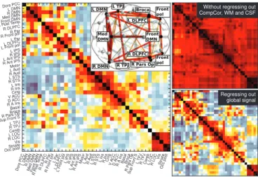
Figure 2: Correlation matrices of rest time-series extracted from the 39 main regions of the Varoquaux 2011 [115] parcellation with differ-ent choices of confound regressors – Left: regressing out CompCor signals, as well as white matter and CSF average signals and move-ment parameters. The insert shows the connections restricted to a few major nodes. – Upper right: regressing out only movement pa-rameters. – Lower right: regressing out movement parameters and global signal mean. No frequency filtering was applied here. When no confounding brain signals are regressed, all regions are heavily cor-related. Regressing out common signal, in the form of well-identified confounds or a global mean, teases out the structure.

though in essence they all strive to extract simple statistics from functional imaging in order to characterize synchrony and communication between large ensembles of neurons. Here we choose to focus on second order statistics that can be related to Gaussian models, the simplest of which being the correlation matrix of the signals of the different ROIs.

Signal extraction. Given a set of graph nodes, the next step is to extract a representative time series for each node. To study intrinsic activity, e.g. with rest data, signal ex-traction can be achieved by either averaging the fMRI time series across the voxels in a region, or by taking the first eigenvariate from a principle components analysis of the

time series [40]. Comparisons of these methods has shown

that the eigenvariate method is more sensitive to function

inhomogeneity [25] and exhibits worse test-retest

reliabil-ity than averaging time series [128]. In addition, improved

specificity to BOLD signal can be enforced by using only signal in voxels near gray-matter tissues. For this pur-pose, we suggest summarizing the signal in an ROI by a mean of the different voxels weighted by the subject-specific gray matter probabilistic segmentation, as output

by e.g. SPM’s segmentation tool [4] or FSL’s FAST

pro-gram [126].

Studying connectivity from evoked activity with task-driven studies requires disambiguating task-specific con-nectivity effects from intrinsic concon-nectivity mediated by shared neuromodulatory/task inputs, anatomical path-ways, etc. In this regard, it can be beneficial to run a GLM-based first-level analysis, enforcing specificity of the measure extracted to the task. With slow event-related

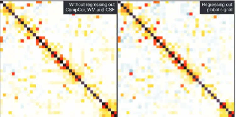
Do rs PC C LD MN RD MN Me dD MN Fro nt DM N RP ost Te mp R DL PF C RP ar RF ron tp ol LP ar LD LP FC LF ron tp ol LIP S R IPS LA nt IPS RA nt IPS Mo tor LA ud R Au d LS TS R ST S LIn s RIn s Cin g VA CC DA CC RA Ins Ba sa l Bro ca R Pa rs Op Su pF ron tS LT PJ R TP J Ce reb LL OC RL OCVis Str iate Occ po st Dors PCC L DMN R DMN Med DMN Front DMN R PostTemp R DLPFC R Par R Front pol L Par L DLPFC L Front pol L IPS R IPS L Ant IPS R AntIPS Motor L Aud R Aud L STS R STS L Ins R Ins Cing V ACC D ACC R A Ins Basal Broca R ParsOp Sup Front S L TPJ R TPJ Cereb L LOC R LOC Vis Striate Occ post Without sparsity GraphLasso estimate

Figure 3: Different inverse-covariance matrices estimates corre-sponding to fig.2 – Left: group-sparse estimate using the ℓ21 es-timator [116]. The insert shows the connections restricted to a few major nodes. – Upper right: non-sparse estimate: inverse of the sample correlation matrix. – Lower right: sparse estimate using the Graph Lasso [34].

designs, task-specific functional connectivity can be cap-tured in trial-to-trial fluctuations in the BOLD response, estimated using a GLM analysis with one regressor per

trial [47,75,86]. This approach, known as beta-series

re-gression, has been adapted for rapid event-related designs, using multiple GLMs to optimize deconvolution of each

trial [76].

Correlation and partial correlations. Given ROIs defining the nodes of the functional-connectome graph, one needs to estimate the corresponding edges connecting them. Functional connectivity between the ROIs can be mea-sured by computing the correlation matrix of the extracted signals. An important and often neglected point is that the sample correlation matrix, i.e. the correlation matrix ob-tained by plugging the observed signal in the correlation matrix formula, is not the population correlation matrix, i.e. the correlation matrix of the data-generating process. If the number of measurements was infinite, the two would coincide, however if this number is not large compared to the number of connections (that scales as the square of the number of ROIs), the sample correlation matrix is a poor estimate of the underlying population correlation matrix. In other words, the sample correlation matrix captures a lot of sampling noise, intrinsic randomness that arises in the estimation of correlations from short time series. Con-clusions drawn from the sample correlation matrix can

eas-ily reflect this estimation error. Varoquaux et al. [116] and

Smith et al. [100] have shown respectively on rest fMRI and

on realistic simulations that a good choice of correlation matrix estimator could recover the connectivity structure, where the sample correlation matrix would fail. In general, the choice of a better estimate depends on the settings and

the end goals [114, 117], however the Ledoit-Wolf

Without regressing out CompCor, WM and CSF

Regressing out global signal

Figure 4: Inverse-covariance matrices for different choice of con-found regressors – Left: regressing out only movement parameters – Right: removal of the global mean, instead of the white matter, CSF, and CompCor time courses.

parameter-less alternative that performs uniformly better

than the sample correlation matrix [116, 117] and should

always be preferred.

For the problem of recovering the

functional-connectivity structure, i.e. finding which region is con-nected to which, sparse inverse covariance estimators have

been found to be efficient [89,100,116]. The intuition for

relying on inverse covariance rather than correlation stems from that fact that standard correlation (marginal correla-tion) between two variables a and b also capture the effects of other variables: strong correlation of a and b with a third variable c will induce a correlation between a and b. On

the opposite, the inverse covariance3 _{matrix (also called}

precision matrix ) captures partial correlations, removing

the effect of other variables [71]. In the small sample limit,

this removal is challenging from the statistical standpoint. This is why an assumption of sparsity, i.e. that only few variables need to be considered at a time, is important to estimate a good inverse covariance. Various estimation strategies exist for sparse inverse covariance, and have an

impact on the resulting networks [116, 117]. The Graph

Lasso (ℓ1-penalized maximum-likelihood estimator) [34] is

in general a good approach for structure recovery. In group

studies, the ℓ21 estimator [50, 116] is useful to impose a

common sparsity structure across different subjects and achieve better recovery of this common structure. Simply put, these approaches are necessary because estimation

noise creates a background structure (see fig.3); however,

unlike in a univariate situation, the parameters are not in-dependent, and the spurious background connections de-grade the estimation of the actual connections. The sparse estimators make a compromise between imposing simpler models, i.e. with less connections, and providing a good fit to the data. This compromise is set via a regulariza-tion parameter which controls the sparsity of the estimate. A good procedure to choose this parameter is via

cross-3

Covariance and correlation matrices differ simply by the fact that a covariance matrix captures the amplitude of a signal, via its variance, while a correlation matrix is computed on standardized (zero mean, unit variance) signals.

validation [116].

Network structure extracted. The correlation matrices and inverse-covariance matrices that we extract contain a lot of information on the functional structure of the brain. First,

the correlation matrix (fig.2) shows blocks of synchronized

regions that can be interpreted as large-scale functional networks, such as the default mode network. Note that the split in networks is not straightforward. Different ordering of the nodes will reveal different networks. Indeed, because of the presence of hubs and interleaved networks, the pic-ture in terms of segregated networks is not sufficient to

ex-plain full-brain connectivity [117]. Connectivity matrices,

correlation matrices and inverse-covariance matrices, can be represented as graphs: nodes connected by weighted

edges (inserts on fig.2 and fig.3). The inverse-covariance

matrix, which captures partial correlations, appears then as extracting a backbone or core of the graph. While such structure has been used as a way to summarize

anatomi-cal brain connectivity graphs [49], here it has a clear-cut

meaning with regard to the BOLD signal: it gives the

con-ditional independence structure between regions [117]. In

other words, regions a and b are not connected if the sig-nal that they have in common can be explained by a third region c. In this light, the choice of nuisance regressors to remove confounding common signal is less critical with partial correlations than with correlations. Indeed, while with correlation matrices regressing out the global mean

has a drastic effect (fig.2 upper right and lower right), on

inverse covariance it only changes the resulting matrices

very slightly (fig.4).

There have been debates on whether to regress out cer-tain signals, such as the global mean, as it induces negative

correlations [19, 32, 77], and these may seem surprising:

one network appears as having opposite fluctuations to another. However, correlation between two signals only takes its meaning with the definition of a baseline. A sim-ple picture to explain anti-correlations between two regions is the presence of a third region, mediating the interac-tions. Using this third region as a baseline would amount to estimate partial correlations in the whole system. Us-ing inverse-covariance matrices or partial correlations to understand brain connectivity makes the interpretation in terms of interactions between brain regions easier and more robust to the choice of confounds.

3. Comparing connectivity

We now turn to the problem of comparing functional connectivity across subjects or across conditions.

3.1. Detecting changing connections

First, we focus on detecting where the connectivity ma-trices estimated in the previous section differ.

Mass-univariate approaches. The most natural approach is to apply a linear model to each coefficient of the

con-nectivity matrices [47,64]. This approach is similar to the

second-level analysis used in mass-univariate brain map-ping, and gives rise to many of the well-known techniques used in such a context, such as the definition of a second-level design, with possibly the inclusion of confounding ef-fects, and statistical tests (T tests or F tests) on contrast vectors. Importantly, in order to work with Gaussian-distributed variables, it is necessary to apply a Fisher Z

transform4 _{to the correlations. Note that in these}

set-tings, the Ledoit-Wolf estimator [62] is often a good choice

to estimate the correlation matrix, as it is parameter-free and gives good estimation performance without imposing any restrictions on the data. For hypothesis testing, cor-recting for multiple comparison can severely limit statis-tical power, as the number of tests performed scales as the square of the number of regions used. Controlling for the false discovery rate (FDR) mitigates this problem. Al-ternatively, as the assumptions underlying the

Benjamini-Hochberg procedure [10] for the FDR can easily be broken,

non-parametric permutations-based tests give reliable

ap-proaches. In particular, the max-T procedure [42, 79] is

interesting to avoid the drastic Bonferroni correction when controlling for multiple comparison in family-wise error rate.

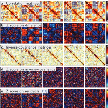
Accounting for distributed variability. A specific challenge of connectivity analysis is that the connectivity strength between different regions tends to covary. For instance, with resting-state data, functional networks comprising many nodes can appear as more or less connected across

subjects (see for instance fig.5, showing variability in a

control population at rest). In other words, non-specific variability is distributed across the connectivity graph,

and it is structured by the graph itself. This

obser-vation brings the natural question of whether second-level analysis should be performed on correlation matri-ces, inverse-covariance matrimatri-ces, or another parametriza-tion that would disentangle effects and give unstructured (white) residuals. While inverse-covariance matrices show less distributed fluctuations than correlation matrices, they capture a lot of background noise, as partial corre-lations are intrinsically harder to estimate. Preliminary

work [114] suggests performing statistical tests on

residu-als of a parametrization intermediate between correlation matrix and inverse covariance matrix, as it can decouple effects and noise.

Taking a different stance on distributed variability, the

“network-based statistics” approach [122] draws from the

hypothesis that if, in a second-level analysis, an effect is detected on a connection that lies in a network of strongly connected nodes, a large sub-network is likely to carry an

4

Seehttp://en.wikipedia.org/wiki/Fisher_transformationor [3] section 4.2.3 for mathematical arguments.

-1 1 a. Correlation matrices -4 4 b. Z score on difference -1 1 c. Inverse-covariance matrices -4 4 d. Z score on inverse-covariance -4 4 e. Z score on residuals[114]

Figure 5: Inter subject variability. Note that this is variability occur-ring in a healthy population at rest, in other words it is non specific variability – a: single-subject correlation matrices for different sub-jects – b: Corresponding Z-score (effect / standard deviation) of the difference between a subject and the remaining others – c: single-subject inverse-covariance matrices – d: Corresponding Z-score for the inverse-covariance matrices – e: Corresponding Z-score for the subject residuals, as defined in [114].

effect. Thus, they adapt cluster-level inference to connec-tivity analysis, in order to mitigate the curse of multiple comparisons.

3.2. Comparing network summary statistics

Both the multiple comparison issue and the network-level distributed variability are a plague to edge-network-level com-parison of connectomes. A possible strategy to circumvent these difficulties is to perform comparisons and statistical testing at the level of the network, rather than the indi-vidual connection.

Network integration. Marrelec et al. [69] introduce the

use of entropy and mutual information as a measure of

network-level functional integration5_{. Gaussian entropy}

can be seen as a simple metric to generalize correlation or

variance to multiple nodes (see [3] §2.5.2 and §7.5).

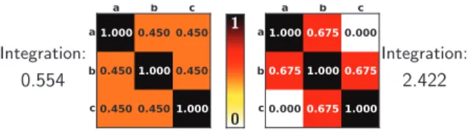
In-deed, let us consider 3 nodes: a, b and c. Their correlation

structure is captured by three correlation coefficients: ρab,

ρbc and ρac. Summarizing these by their mean, as might

seem natural, discards the relationship between the sig-nals, while using the integration metric, defined as the Gaussian entropy, tells us how much two signals can be

5

See [116] for simplified formulas for network integration and mu-tual information.

Integration: 0.554 0 1 Integration: 2.422

Figure 6: Two different correlation matrices with the same average correlation, but with very different integration values. Indeed, the matrix on the left was chosen to represent three signals a, b and c as different from each other as possible, given ρab+ ρbc+ ρac_{= 1.35; it} thus has a small integration value. On the opposite, for the matrix on the right, signal b can almost be fully recovered by combining signals a and c; the matrix thus has a large integration value.

combined to form the third (see fig.6). Cross-entropy –or

mutual information– [69] measures the amount of

cross-talk between two systems in a similar way as Gaussian entropy is used to measure the integration of a brain sys-tem. The functional-connectivity structure, or its repre-sentation in the form of a correlation matrix, can thus be characterized via the integration and cross-talk of some of its sub-systems. This approach gives a simplified rep-resentation with a small number of metrics that can be compared across subjects.

Graph-topological metrics. Functional connectivity graphs have been found to display specific topological

prop-erties6 _{that are characteristic of small-world networks}

[1,17,91,103]. These networks display excellent transport

properties: although they have a relatively small number of connections, any two regions of the brain are well con-nected. Another interesting consequence of their specific topology is the resilience it gives the system to attacks such

as resulting from brain lesions [1]. This overall structure

of functional-connectivity graphs can be summarized by a few metrics, such as the average path length between any two nodes, the local clustering coefficients, or the

node degree centrality [87]. Given that pathologies

with-out a localized focus, such as schizophrenia, are thought

to have a global impact on brain connectivity [5, 65], the

graph-topological metrics are promising markers to per-form inter-subject comparison. Such an approach is ap-pealing as it is not subject to multiple comparison issues. However, it has been criticized as giving a fairly unspe-cific characterization of the brain and being fragile to noise

[54]. Another caveat is that these properties are not

spe-cific to brain function: correlation matrices display small-world properties such as local clustering by construction. Indeed, if two nodes are strongly correlated to a third,

they are highly likely to be correlated to each other [123].

This observation highlights the need for well defined

null-hypothesis [88, 123], but also for controlled recovery of

brain functional connectivity going beyond empirical cor-relation matrices, as discussed in the previous section.

6

In the neuroscience world, these descriptions are grouped under the terms of “graph-theoretical approaches”, however graph theory is an entire division of mathematics and computer science that is concerned with much more than topology of random graphs.

3.3. Predictive Modeling

Predictive modeling is concerned with learning (or fit-ting) a model that is capable of predicting information

from unseen data [80]. In the context of connectomes,

pre-dictive modeling can extract connectivity-based biomark-ers of disease diagnosis, prognosis, or other phenotypic

outcomes [24, 27]. The accuracy of a predictive model

provides a measure of the amount of information present in the connectome about the phenotypic measure being

evaluated [58, 59]. When combined with reproducibility,

prediction accuracy provides a metric for evaluating ex-perimental trade-offs for data acquisition, preprocessing,

and analysis [60, 106]. Multivariate predictive models are

attractive in connectomics because they are sensitive to dependencies between features and avoid the need to cor-rect for multiple comparisons since the significance of an entire pattern is evaluated using a single statistical test. Additionally, modern predictive modeling techniques draw from the statistical learning literature, which specifically addresses high dimensional datasets with few observations. Predictive modeling has been successfully applied to iden-tify connectome-based biomarkers of Alzheimer’s disease

[104], depression [24, 125], schizophrenia [18, 94], autism

[2], ADHD [127], aging [27], as well as to classify mental

operations [85,95]. The growing interest for applying

pre-dictive modeling to connectivity analysis was highlighted by the ADHD200 Global Competition, in which the object was to identify a connectivity-based biomarker of ADHD

[108]. Recent work has illustrated the utility of predictive

modeling for deriving connectivity models at the

individ-ual level [22].

Technically, predictive modeling is a supervised ma-chine learning problem where a target to be predicted –e.g. age, disease state, cognitive state– is available for each observation of the data. In the context of comparing connectomes, features used in the predictive model

corre-spond to bivariate measures of connectivity [27, 85, 95],

or any of the previously discussed graph summary metrics

[18,29]. The quality of a predictive model is determined by

its prediction accuracy (or generalization ability) which is measured using one or more iterations of cross-validation. Cross-validation iteratively subdivides available data into a subset used for training the classifier and a dataset for

evaluating classifier performance7_{[80]. The significance of}

achieved prediction accuracy can be assessed using

permu-tation tests [44]. Predictive modeling approaches typically

require the specification of several parameters, which may be chosen based on domain specific knowledge or

require-ments [21], determined using an analytical approach [20],

or optimized using a second-level cross validation

proce-dure [33].

7

Several strategies exist for performing cross-validation and the commonly used approach of using only a single observation for testing (leave-one-out cross-validation) results in highly variable estimates of prediction accuracy [33]. Alternative approaches such as (5 or 10)-fold cross-validation, or 0.632+ bootstrap should be preferred [33].

Although predictive modeling techniques are well suited for measuring whether information exists in the con-nectome about a phenotypic variable, they do not directly identify the connections that are most relevant to the pre-diction. This limitation can be somewhat mitigated by relying on previously described sparse inverse covariance estimation techniques to minimize the number of

connec-tions. Additionally, feature selection [48] can be performed

by filtering out features based on their statistical

relation-ship with the variable of interest [24,94]. Importantly, it

must be performed within cross-validation to avoid bias-ing estimates of prediction accuracy. The interpretation of connections used in predictive models and their relation-ship with a phenotypic outcome is difficult and requires insight into the mechanisms underlying the modeling ap-proach. For linear models, the weights of the model are similar to the weights of an ordinary linear regression. If features are appropriately standardized prior to training, the magnitude of the weights can be interpreted to re-flect the relative importance of the feature to the model, for instance the corresponding edge in the connectome. However, interpreting how the connections differ between classes or relate to a phenotypic variable can be more com-plicated given the multivariate nature of their involvement. Indeed, the inclusion or exclusion of a connection in the model can induce a change of the sign of another model

weight [24]. It is perhaps most reasonable to adapt a

con-servative interpretation in which predictive modeling is used to identify candidate connections that are later tested in follow-up experiments better suited to elucidating their relationship to the variable of interest.

To conclude on predictive modeling with a practical note for connectome comparison, we would like to stress that while machine learning algorithms are powerful tools, they work best if they are provided with discriminant-ing and noiseless features. In other words, as with all other connectome comparison methods, optimizing first-level analysis –subject-first-level connectome extraction– is paramount.

4. Beyond correlation, effective connectivity? All the approaches that we have presented in this re-view are based on second-order statistics of the signal, in other words correlation analysis. Traditionally, these are defined as functional connectivity, defined as “tempo-ral correlations between remote neurophysiological events”

[35], and opposed to effective connectivity, i.e. “the

in-fluence one neural system exerts over another” [35]. To

conclude this review, we would like to bridge the gap be-tween these concepts, which in our eyes should be seen as a continuum rather than an opposition (this opinion is also

expressed in [73]).

A first step to move from purely descriptive statistics to interaction models with functional connectivity analysis is to consider a correlation matrix as a Gaussian graphi-cal model, i.e. a well-defined probabilistic model that

de-scribes observed correlations in terms of an independence

structure and conditional relations [61,117]. In such

set-tings, the inverse covariance graph or the partial correla-tions are a measure of influence from one node to another, albeit undirected. Inferring directionality in a Gaussian model is impossible. Linear structural equation models

(SEMs) [74] rely on a similar model that consists in

speci-fying a candidate directed graphical structure. This struc-ture constraints the covariance matrix of the signals and can thus be tested on observed data. In fact some forms of SEMs are known as “covariance structure models”. There is thus a strong formal link between correlation analysis in the framework of graphical models and SEMs: the former is undirected but fully exploratory, as it does not require the specification of candidate structure, while the latter is directed but confirmatory. This link has been exploited to specify candidate structures for SEMs using partial

cor-relations [70]. More complex models, such as dynamical

causal models (DCMs) [38] or Granger causality [43]

re-quire additional hypotheses such as non-linear couplings or time lags.

Most importantly, more complex models can only be used to model interactions between a small number of nodes. This is not only due to a computational difficulty, but also to fundamental roadblocks in statistics: the com-plexity of the model must match the richness of the data. While injecting prior information can help model estima-tion, the more informative this prior is, the more fragile the inference becomes. The ongoing debate on the impact

of hemodynamic lag on Granger-causality inference [96]

is an example of such fragility. Note that although most of the theory underpinning correlation analysis (Gaussian graphical models) is based on a Gaussian assumption, the

core results are robust to violations of this assumption [84].

It is tempting to favor more neurobiologically-inspired models that give descriptions close to our knowledge of the brain basic mechanisms, however, as George Box famously said, “all models are wrong; some models are useful”. De-pending on the question and the data at hand, a trade-off should be chosen between complex models based on a bio-physical description, and simple phenomenological models such as correlation matrices. In particular to model inter-actions between a large number of regions, as in full-brain analysis, and learn a large connectome, simple models are to be preferred. For more hypothesis-driven studies, such as the analysis of the mechanisms underlying a specific task, more complex models can be preferred, if rich data is available. Automatic choice of model is a difficult

prob-lem, however, cross-validation (as used in [25, 105, 116])

is a useful tool. The central principle of cross-validation is to test a model on different data than the data used to fit the model. Models too complex for the data available will fit noise in the data, and thus generalize poorly. The main benefit of cross-validation is that it is a non-parametric method which does not rely strongly on modeling

assump-tions8_.

5. Conclusion

Horwitz el al. [52] claimed almost 20 years ago that

“the crucial concept needed for network analysis is covari-ance”. In our eyes, this still holds today. Estimation func-tional connectomes relies largely on fitting covariance mod-els. Their comparison requires understanding how these covariances vary and finding metrics to capture this vari-ability. The additional secret ingredient may be using con-founds regressors in all statistical steps. A good choice of a small number of relevant regions facilitates connectome comparison. However, such a choice cannot yet be fully factored out via methods and must rely on neuroscientific expertise.

Methodological challenges to functional-connectome-based group studies arise from the dimensionality and

the variability of the connectome. With the current

tools, inter-subject comparison of connectomes compris-ing many nodes is limited by the difficulty of estimatcompris-ing high-dimensional covariance matrices and the loss of sta-tistical power due to multiple comparisons. Better algo-rithms integrating powerful a priori information are re-quired to push the limits of covariance estimation. Better characterization of inter-subject variability of connectomes

[56] will help choosing parameterizations and invariants to

avoid testing each edge for a difference, as this strategy inevitably leads to a needle in a haystack problem.

Reviewing methodological options to learn and com-pare connectomes highlights that there is currently no unique solution, but a spectrum of related methods and analytical strategies. More empirical results are required to guide the choices. However this diversity is probably unavoidable: a diffuse disease like schizophrenia will not lead to the same connectome modifications as a focal

le-sion. In statistical learning, “no free lunch” theorems [120]

tell us that no strategy can perform uniformly better in all situations. In practice, the key to a successful analysis is to understand well the assumptions and interpretation of each option, in order to match the method to the question. Similarly, the idealized notion of an unique functional con-nectome to describe connections in brain function is prob-ably an utopia, and various connectomes should be con-sidered in different settings, such as the study of varying

8

This is to be contrasted to Bayesian model comparison, which will give well-controlled results only if the true generative model is in the list of models compared. [36] argues that, based on the Neyman-Pearson lemma, cross-validation is less powerful than likelihood ratio tests using the full dataset. However, it is important to keep in mind that these approaches only test for self-consistence, as the Neyman-Pearson lemma is established under the hypothesis that the model used to define the test is indeed the data-generating process [78], while in practice it is often the case that this model gives poor fits to the data [66]. Applying test procedures on different data than that used to fit the model, as in cross-validation, is much more resilient to modeling errors.

phenotypic conditions, or that of on-going activity versus activity related to specific tasks.

Acknowledgments

GV acknowledges funding from the NiConnect grant and the Dynamic Diaschisis project DEQ20100318254 from Fondation pour la Recherche M´edicale, as well as many insightful discussions with Andreas Kleinschmidt on on-going activity and Bertrand Thirion on statistical data processing. RCC would like to acknowledge support by a NARSAD Young Investigator Grant from the Brain & Behavior Research Foundation. The authors would like to thank the anonymous reviewers for their suggestions, which improved the manuscript.

References

[1] S. Achard, R. Salvador, B. Whitcher, J. Suckling, E. Bullmore, A resilient, low-frequency, small-world human brain functional network with highly connected association cortical hubs, J Neurosci 26 (2006) 63.

[2] J. Anderson, J. Nielsen, A. Froehlich, M. DuBray, T. Druz-gal, A. Cariello, J. Cooperrider, B. Zielinski, C. Ravichandran, P. Fletcher, et al., Functional connectivity magnetic resonance imaging classification of autism, Brain 134 (2011) 3739. [3] T. Anderson, An introduction to multivariate statistical

anal-ysis, Wiley New York, 1958.

[4] J. Ashburner, K. Friston, Unified segmentation, Neuroimage 26 (2005) 839.

[5] D. Bassett, E. Bullmore, B. Verchinski, V. Mattay, D. Wein-berger, A. Meyer-Lindenberg, Hierarchical organization of hu-man cortical networks in health and schizophrenia, J Neurosci 28 (2008) 9239.

[6] C.F. Beckmann, S.M. Smith, Probabilistic independent com-ponent analysis for functional magnetic resonance imaging, Trans Med Im 23 (2004) 137.

[7] Y. Behzadi, K. Restom, J. Liau, T. Liu, A component based noise correction method (compcor) for bold and perfusion based fMRI, Neuroimage 37 (2007) 90.

[8] P. Bellec, V. Perlbarg, S. Jbabdi, M. Pelegrini-Issac, J.L. An-ton, J. Doyon, H. Benali, Identification of large-scale networks in the brain using fMRI., Neuroimage 29 (2006) 1231. [9] P. Bellec, P. Rosa-Neto, O. Lyttelton, H. Benali, A. Evans,

Multi-level bootstrap analysis of stable clusters in resting-state fMRI, NeuroImage 51 (2010) 1126.

[10] Y. Benjamini, Y. Hochberg, Controlling the false discovery rate: a practical and powerful approach to multiple testing, J Roy Stat Soc B (1995) 289.

[11] R.M. Birn, J.B. Diamond, M. Smith, P. Bandettini, Separat-ing respiratory-variation-related fluctuations from neuronal-activity-related fluctuations in fMRI, NeuroImage 31 (2006) 1536.

[12] R.M. Birn, M. Smith, T.B. Jones, P. Bandettini, The respira-tion response funcrespira-tion: the temporal dynamics of fMRI signal fluctuations related to changes in respiration, NeuroImage 40 (2008) 644.

[13] B. Biswal, M. Mennes, X. Zuo, S. Gohel, C. Kelly, S. Smith, C. Beckmann, et al., Toward discovery science of human brain function, Proc Ntl Acad Sci 107 (2010) 4734.

[14] B. Biswal, F. Zerrin Yetkin, V. Haughton, J. Hyde, Functional connectivity in the motor cortex of resting human brain using echo-planar MRI, Magn Reson Med 34 (1995) 53719. [15] T. Blumensath, T.E.J. Behrens, S.M. Smith, Resting-state

fMRI single subject cortical parcellation based on region grow-ing, MICCAI (2012) 188.

[16] R. Boyacio˘glu, M. Barth, Generalized iNverse imaging (GIN): Ultrafast fMRI with physiological noise correction, Mag Res Med (2012) epub ahead of print.

[17] E. Bullmore, O. Sporns, Complex brain networks: graph theo-retical analysis of structural and functional systems, Nat Rev Neurosci 10 (2009) 186.

[18] G. Cecchi, I. Rish, B. Thyreau, B. Thirion, M. Plaze, M. Paillere-Martinot, C. Martelli, J. Martinot, J. Poline, Dis-criminative network models of schizophrenia, in: Advances in Neural Information Processing Systems, 2009.

[19] C. Chang, G. Glover, Effects of model-based physiological noise correction on default mode network anti-correlations and correlations, Neuroimage 47 (2009) 1448.

[20] V. Cherkassky, Y. Ma, Practical selection of SVM parame-ters and noise estimation for svm regression, Neural Netw. 17 (2004) 113.

[21] V. Cherkassky, F. Mulier, Learning from Data: Concepts, The-ory, and Methods, John Wiley & Sons, 1998.

[22] C. Chu, D.A. Handwerker, P.A. Bandettini, J. Ashburner, Measuring the consistency of global functional connectivity using kernel regression methods, in: Proceedings of the 2011 IEEE International Workshop on Pattern Recognition in Neu-roImaging, p. 41.

[23] D. Cordes, V. Haughton, K. Arfanakis, J. Carew, P. Turski, C. Moritz, M. Quigley, M. Meyerand, Frequencies contributing to functional connectivity in the cerebral cortex in “resting-state” data, Am J Neuroradio 22 (2001) 1326.

[24] R. Craddock, P. Holtzheimer III, X. Hu, H. Mayberg, Dis-ease state prediction from resting state functional connectivity, Magnetic resonance in Medicine 62 (2009) 1619.

[25] R. Craddock, G. James, P. Holtzheimer III, X. Hu, H. May-berg, A whole brain fMRI atlas generated via spatially con-strained spectral clustering, Hum Brain Mapp 33 (2012) 1914. [26] C. Davey, D. Grayden, G. Egan, L. Johnston, Filtering induces correlation in fMRI resting state data, NeuroImage 64 (2013) 728.

[27] N. Dosenbach, B. Nardos, A. Cohen, D. Fair, J. Power, J. Church, S. Nelson, G. Wig, A. Vogel, C. Lessov-Schlaggar, et al., Prediction of individual brain maturity using fmri, Sci-ence 329 (2010) 1358.

[28] N.U. Dosenbach, K.M. Visscher, E.D. Palmer, F.M. Miezin, K.K. Wenger, H.C. Kang, E.D. Burgund, A.L. Grimes, B.L. Schlaggar, S.E. Petersen, A core system for the implementation of task sets, Neuron 50 (2006) 799.

[29] M. Ekman, J. Derrfuss, M. Tittgemeyer, C. Fiebach, Predict-ing errors from reconfiguration patterns in human brain net-works, P Natl Acad Sci Usa (2012) epub ahead of print. [30] M. Fox, M. Greicius, Clinical applications of resting state

func-tional connectivity, Frontiers in systems neuroscience 4 (2010). [31] M. Fox, A. Snyder, J. Vincent, M. Corbetta, D. Van Essen, M. Raichle, The human brain is intrinsically organized into dynamic, anticorrelated functional networks, Proc Ntl Acad Sci 102 (2005) 9673.

[32] M. Fox, D. Zhang, A. Snyder, M. Raichle, The global sig-nal and observed anticorrelated resting state brain networks, J Neurophysio 101 (2009) 3270.

[33] J. Friedman, T. Hastie, R. Tibshirani, The elements of statis-tical learning, Springer Series in Statistics, 2001.

[34] J. Friedman, T. Hastie, R. Tibshirani, Sparse inverse covari-ance estimation with the graphical lasso, Biostatistics 9 (2008) 432.

[35] K.J. Friston, Functional and effective connectivity in neu-roimaging: a synthesis, Hum Brain Mapp 2 (1994) 56. [36] K.J. Friston, Ten ironic rules for non-statistical reviewers,

Neu-roImage 61 (2012) 1300.

[37] K.J. Friston, C.D. Frith, P.F. Liddle, R.S.J. Frackowiak, Functional connectivity: the principal-component analysis of large (PET) data sets, Journal of cerebral blood flow and metabolism 13 (1993) 5.

[38] K.J. Friston, L. Harrison, W. Penny, Dynamic causal mod-elling., Neuroimage 19 (2003) 1273.

[39] K.J. Friston, A.P. Holmes, K.J. Worsley, J.B. Poline, C. Frith, R.S.J. Frackowiak, Statistical parametric maps in functional imaging: A general linear approach, Hum Brain Mapp (1995) 189.

[40] K.J. Friston, P. Rotshtein, J.J. Geng, P. Sterzer, R.N. Henson, A critique of functional localisers, Neuroimage 30 (2006) 1077. [41] K.J. Friston, S. Williams, R. Howard, R.S. Frackowiak, R. Turner, Movement-related effects in fMRI time-series, Mag-netic resonance in medicine 35 (1996) 346.

[42] Y. Ge, S. Dudoit, T. Speed, Resampling-based multiple testing for microarray data analysis, Test 12 (2003) 1.

[43] R. Goebel, A. Roebroeck, D. Kim, E. Formisano, Investigating directed cortical interactions in time-resolved fmri data using vector autoregressive modeling and granger causality mapping, Magnetic resonance imaging 21 (2003) 1251.

[44] P. Golland, B. Fischl, Permutation tests for classification: To-wards statistical significance in image-based studies., in: IPMI, p. 330.

[45] M. Greicius, Resting-state functional connectivity in neuropsy-chiatric disorders, Current opinion in neurology 21 (2008) 424. [46] M. Greicius, B. Krasnow, A. Reiss, V. Menon, Functional con-nectivity in the resting brain: a network analysis of the default mode hypothesis, Proc Ntl Acad Sci 100 (2003) 253.

[47] M.L. Grillon, C. Oppenheim, G. Varoquaux, F. Charbonneau, A. Devauchelle, M. Krebs, F. Bayle, B. Thirion, C. Huron, Hyperfrontality and hypoconnectivity during refreshing in schizophrenia, Psychiatry Research: Neuroimaging (2012). [48] I. Guyon, A. Elisseeff, An introduction to variable and feature

selection, J. Mach. Learn. Res. 3 (2003) 1157.

[49] P. Hagmann, L. Cammoun, X. Gigandet, R. Meuli, C.J. Honey, V.J. Wedeen, O. Sporns, Mapping the structural core of human cerebral cortex, PLoS Biol 6 (2008) e159.

[50] J. Honorio, D. Samaras, Simultaneous and group-sparse multi-task learning of gaussian graphical models, arXiv:1207.4255 (2012).

[51] B. Horwitz, The elusive concept of brain connectivity, Neu-roImage 19 (2003) 466.

[52] B. Horwitz, A. McIntosh, J. Haxby, C. Grady, Network analy-sis of brain cognitive function using metabolic and blood flow data, Behavioural brain research 66 (1995) 187.

[53] X. Hu, T.H. Le, T. Parrish, P. Erhard, Retrospective estima-tion and correcestima-tion of physiological fluctuaestima-tion in funcestima-tional MRI, Magn Reson Med 34 (1995) 201.

[54] A. Ioannides, Dynamic functional connectivity, Current opin-ion in neurobiology 17 (2007) 161.

[55] H.J. Jo, Z.S. Saad, W.K. Simmons, L.a. Milbury, R.W. Cox, Mapping sources of correlation in resting state FMRI, with artifact detection and removal, NeuroImage 52 (2010) 571. [56] C. Kelly, B. Biswal, R. Craddock, F. Castellanos, M.

Mil-ham, Characterizing variation in the functional connectome: promise and pitfalls, Trends in cognitive sciences 16 (2012) 181.

[57] V. Kiviniemi, T. Starck, J. Remes, X. Long, J. Nikkinen, M. Haapea, J. Veijola, et al., Functional segmentation of the brain cortex using high model order group PICA., Hum Brain Map 30 (2009) 3865.

[58] U. Kjems, L. Hansen, J. Anderson, S. Frutiger, S. Muley, J. Sidtis, D. Rottenberg, S. Strother, The quantitative eval-uation of functional neuroimaging experiments: Mutual infor-mation learning curves, NeuroImage 15 (2002) 772.

[59] N. Kriegeskorte, R. Goebel, P. Bandettini, Information-based functional brain mapping, Proc Ntl Acad Sci 103 (2006) 3863. [60] S. LaConte, J. Anderson, S. Muley, J. Ashe, S. Frutiger, K. Rehm, L. Hansen, E. Yacoub, X. Hu, D. Rottenberg, The evaluation of preprocessing choices in single-subject bold fMRI using npairs performance metrics, NeuroImage 18 (2003) 10. [61] S. Lauritzen, Graphical models, Oxford University Press, USA,

1996.

[62] O. Ledoit, M. Wolf, A well-conditioned estimator for large-dimensional covariance matrices, J. Multivar. Anal. 88 (2004) 365.

[63] L. Lee, L.M. Harrison, A. Mechelli, et al., A report of the func-tional connectivity workshop, dusseldorf 2002, Neuroimage 19 (2003) 457.

[64] C. Lewis, A. Baldassarre, G. Committeri, G. Romani, M. Cor-betta, Learning sculpts the spontaneous activity of the resting human brain, Proc Ntl Acad Sci 106 (2009) 17558.

[65] Y. Liu, M. Liang, Y. Zhou, Y. He, Y. Hao, M. Song, C. Yu, H. Liu, Z. Liu, T. Jiang, Disrupted small-world networks in schizophrenia, Brain 131 (2008) 945.

[66] G. Lohmann, K. Erfurth, K. M¨uller, R. Turner, Critical com-ments on dynamic causal modelling, Neuroimage 59 (2012) 2322.

[67] T.E. Lund, K.H. Madsen, K. Sidaros, W.L. Luo, T.E. Nichols, Non-white noise in fMRI: does modelling have an impact?, NeuroImage 29 (2006) 54.

[68] G. Marrelec, P. Bellec, H. Benali, Exploring large-scale brain networks in functional MRI, J Physio Paris 100 (2006) 171. [69] G. Marrelec, P. Bellec, A. Krainik, H. Duffau, M. P´el´

egrini-Issac, S. Leh´ericy, H. Benali, J. Doyon, Regions, systems, and the brain: hierarchical measures of functional integration in fMRI, Medical Image Analysis 12 (2008) 484.

[70] G. Marrelec, H. Horwitz, J. Kim, M. P´el´egrini-Issac, H. Benali, J. Doyon, Using partial correlation to enhance structural equa-tion modeling of funcequa-tional MRI data., Magn Reson Imaging 25 (2007) 1181.

[71] G. Marrelec, A. Krainik, H. Duffau, M. P´el´egrini-Issac, S. Leh´ericy, J. Doyon, H. Benali, Partial correlation for func-tional brain interactivity investigation in funcfunc-tional MRI, Neu-roimage 32 (2006) 228.

[72] A. McIntosh, Towards a network theory of cognition, Neural Networks 13 (2000) 861.

[73] A. McIntosh, Moving between functional and effective connec-tivity, in: O. Sporns (Ed.), Analysis and Function of Large-Scale Brain Networks, Society for Neuroscience, 2010, p. 15. [74] A. McIntosh, F. Gonzalez-Lima, Structural equation

model-ing and its application to network analysis in functional brain imaging, Hum Brain Map 2 (1994) 2.

[75] M. Mennes, C. Kelly, X.N. Zuo, A. Di Martino, B.B. Biswal, F.X. Castellanos, M.P. Milham, Inter-individual differences in resting-state functional connectivity predict task-induced BOLD activity, Neuroimage 50 (2010) 1690.

[76] J. Mumford, B. Turner, F. Ashby, R. Poldrack, Deconvolving bold activation in event-related designs for multivoxel pattern classification analyses, NeuroImage 59 (2012) 2636.

[77] K. Murphy, R. Birn, D. Handwerker, J. T.B., P. Bandettini, The impact of global signal regression on resting state corre-lations: are anti-correlated networks introduced?, NeuroImage 44 (2009) 893.

[78] J. Neyman, E. Pearson, On the problem of the most efficient tests of statistical hypotheses, Philosophical Transactions of the Royal Society of London. Series A 231 (1933) 289. [79] T. Nichols, A. Holmes, Nonparametric permutation tests for

functional neuroimaging: a primer with examples, Hum brain map 15 (2001) 1.

[80] F. Pereira, T. Mitchell, M. Botvinick, Machine learning clas-sifiers and fmri: a tutorial overview, Neuroimage 45 (2009) S199.

[81] R. Poldrack, J. Mumford, T. Nichols, Handbook of functional MRI data analysis, Cambridge University Press, 2011. [82] J. Power, K. Barnes, A. Snyder, B. Schlaggar, S. Petersen,

Spurious but systematic correlations in functional connectivity mri networks arise from subject motion, Neuroimage 59 (2011) 2142.

[83] M. Raichle, Two views of brain function, Trends in cognitive sciences 14 (2010) 180.

[84] P. Ravikumar, M. Wainwright, G. Raskutti, B. Yu, High-dimensional covariance estimation by minimizing 1-penalized log-determinant divergence, Elec J Stat 5 (2011) 935. [85] J. Richiardi, H. Eryilmaz, S. Schwartz, P. Vuilleumier, D. Van

De Ville, Decoding brain states from fMRI connectivity graphs, NeuroImage 56 (2011) 616.

[86] J. Rissman, A. Gazzaley, M. D’Esposito, Measuring functional connectivity during distinct stages of a cognitive task, Neu-roimage 23 (2004) 752.

[87] M. Rubinov, O. Sporns, Complex network measures of brain connectivity: uses and interpretations, Neuroimage 52 (2010) 1059.

[88] M. Rubinov, O. Sporns, Weight-conserving characterization of complex functional brain networks, Neuroimage 56 (2011) 2068.

[89] S. Ryali, T. Chen, K. Supekar, V. Menon, Estimation of func-tional connectivity in fMRI data using stability selection-based sparse partial correlation with elastic net penalty, Neuroimage 59 (2012) 3852.

[90] Z.S. Saad, S.J. Gotts, K. Murphy, G. Chen, H.J. Jo, A. Mar-tin, R.W. Cox, Trouble at rest: how correlation patterns and group differences become distorted after global signal regres-sion, Brain Connect 2 (2012) 25–32.

[91] R. Salvador, J. Suckling, M. Coleman, Neurophysiological ar-chitecture of functional magnetic resonance images of human brain, Cerebral Cortex 15 (2005) 1332.

[92] T. Satterthwaite, M. Elliott, R. Gerraty, K. Ruparel, J. Loug-head, M. Calkins, S. Eickhoff, et al., An improved framework for confound regression and filtering for control of motion ar-tifact in the preprocessing of resting-state functional connec-tivity data, NeuroImage 64 (2013).

[93] J. Schoffelen, J. Gross, Source connectivity analysis with MEG and EEG, Hum brain map 30 (2009) 1857.

[94] H. Shen, L. Wang, Y. Liu, D. Hu, Discriminative analysis of resting-state functional connectivity patterns of schizophre-nia using low dimensional embedding of fMRI, Neuroimage 49 (2010) 3110.

[95] W. Shirer, S. Ryali, E. Rykhlevskaia, V. Menon, M. Greicius, Decoding subject-driven cognitive states with whole-brain con-nectivity patterns, Cerebral Cortex 22 (2012) 158.

[96] S. Smith, P. Bandettini, K. Miller, T. Behrens, K. Friston, O. David, T. Liu, M. Woolrich, T. Nichols, The danger of systematic bias in group-level FMRI-lag-based causality esti-mation, Neuroimage 59 (2012) 1228.

[97] S. Smith, P. Fox, K. Miller, D. Glahn, P. Fox, C. Mackay, et al., Correspondence of the brain’s functional architecture during activation and rest, Proc Natl Acad Sci 106 (2009) 13040. [98] S. Smith, M. Jenkinson, M. Woolrich, C. Beckmann,

T. Behrens, H. Johansen-Berg, P. Bannister, M.D. Luca, I. Drobnjak, D. Flitney, R. Niazy, J. Saunders, J. Vickers, Y. Zhang, N.D. Stefano, J. Brady, P. Matthews, Advances in functional and structural MR image analysis and implementa-tion as FSL, NeuroImage 23 (2004) 208.

[99] S. Smith, K. Miller, S. Moeller, J. Xu, E. Auerbach, M. Wool-rich, C. Beckmann, M. Jenkinson, J. Andersson, M. Glasser, et al., Temporally-independent functional modes of sponta-neous brain activity, Proc Ntl Acad Sci 109 (2012) 3131. [100] S. Smith, K. Miller, G. Salimi-Khorshidi, M. Webster, C.

Beck-mann, T. Nichols, J. Ramsey, M. Woolrich, Network modelling methods for fMRI, Neuroimage 54 (2011) 875.

[101] O. Sporns, D. Chialvo, M. Kaiser, C. Hilgetag, Organization, development and function of complex brain networks, Trends in Cognitive Sciences 8 (2004) 418.

[102] O. Sporns, G. Tononi, R. Kotter, The human connectome: a structural description of the human brain, PLoS Comput Biol 1 (2005) e42.

[103] C. Stam, Functional connectivity patterns of human mag-netoencephalographic recordings: a “small-world” network?, Neuroscience letters 355 (2004) 25.

[104] C. Stonnington, C. Chu, S. Kl¨oppel, C. Jack Jr, J. Ashburner, R. Frackowiak, et al., Predicting clinical scores from magnetic resonance scans in alzheimer’s disease, Neuroimage 51 (2010) 1405.

[105] S. Strother, Evaluating fMRI preprocessing pipelines, Engi-neering in Medicine and Biology Magazine, IEEE 25 (2006) 27.

Kus-tra, J. Sidtis, S. Frutiger, S. Muley, S. LaConte, D. Rottenberg, The quantitative evaluation of functional neuroimaging exper-iments: the NPAIRS data analysis framework, Neuroimage 15 (2002) 747.

[107] J. Talairach, P. Tournoux, Co-planar Stereotaxic Atlas of the Human Brain: 3-dimensional Proportional System, Thieme Classics, Thieme Medical Pub, 1988.

[108] The ADHD-200 Consortium, The ADHD-200 consortium: A model to advance the translational potential of neuroimaging in clinical neuroscience, Front Syst Neurosci 6 (2012) 62. [109] B. Thirion, G. Flandin, P. Pinel, A. Roche, P. Ciuciu, J.B.

Poline, Dealing with the shortcomings of spatial normalization: Multi-subject parcellation of fMRI datasets, Hum brain map 27 (2006) 678.

[110] G. Tononi, O. Sporns, G. Edelman, Reentry and the problem of integrating multiple cortical areas: simulation of dynamic integration in the visual system, Cerebral Cortex 2 (1992) 310. [111] N. Tzourio-Mazoyer, B. Landeau, D. Papathanassiou, F. Criv-ello, O. Etard, N. Delcroix, B. Mazoyer, M. Joliot, Automated anatomical labeling of activations in SPM using a macroscopic anatomical parcellation of the MNI MRI single-subject brain., Neuroimage 15 (2002) 273.

[112] K. Van Dijk, M. Sabuncu, R. Buckner, The influence of head motion on intrinsic functional connectivity MRI, Neuroimage 59 (2012) 431.

[113] E. Van Oort, D. Norris, S. Smith, C. Beck-mann, Resting state networks are character-ized by high frequency BOLD fluctuations,

https://ww4.aievolution.com/hbm1201/index.cfm?do=abs.viewAbs&abs=6235, 2012.

[114] G. Varoquaux, F. Baronnet, A. Kleinschmidt, P. Fillard, B. Thirion, Detection of brain functional-connectivity differ-ence in post-stroke patients using group-level covariance mod-eling, in: MICCAI, 2010.

[115] G. Varoquaux, A. Gramfort, F. Pedregosa, V. Michel, B. Thirion, Multi-subject dictionary learning to segment an atlas of brain spontaneous activity, in: Inf Proc Med Imag, p. 562.

[116] G. Varoquaux, A. Gramfort, J.B. Poline, B. Thirion, Brain covariance selection: better individual functional connectivity models using population prior, in: NIPS, 2010.

[117] G. Varoquaux, A. Gramfort, J.B. Poline, B. Thirion, Markov models for fMRI correlation structure: is brain functional connectivity small world, or decomposable into networks?, J Physio Paris 106 (2012) 212.

[118] G. Varoquaux, A. Gramfort, B. Thirion, Small-sample brain mapping: sparse recovery on spatially correlated designs with randomization and clustering, ICML (2006).

[119] J. Wang, L. Wang, Y. Zang, H. Yang, H. Tang, Parcellation-dependent small-world brain functional networks: A resting-state fMRI study, Hum Brain Mapp 30 (2009) 1511.

[120] D. Wolpert, The lack of a priori distinctions between learning algorithms, Neural Computation 8 (1996) 1341.

[121] B. Yeo, F. Krienen, J. Sepulcre, M. Sabuncu, et al., The or-ganization of the human cerebral cortex estimated by intrinsic functional connectivity, J Neurophysio 106 (2011) 1125. [122] A. Zalesky, A. Fornito, E. Bullmore, Network-based

statis-tic: Identifying differences in brain networks, NeuroImage 53 (2010) 1197.

[123] A. Zalesky, A. Fornito, E. Bullmore, On the use of correlation as a measure of network connectivity, NeuroImage 60 (2012) 2096.

[124] A. Zalesky, A. Fornito, I.H. Harding, L. Cocchi, M. Y¨ucel, C. Pantelis, E.T. Bullmore, Whole-brain anatomical networks: does the choice of nodes matter?, Neuroimage 50 (2010) 970. [125] L.L. Zeng, H. Shen, L. Liu, L. Wang, B. Li, P. Fang, Z. Zhou,

Y. Li, D. Hu, Identifying major depression using whole-brain functional connectivity: a multivariate pattern analysis, Brain 135 (2012) 1498.

[126] Y. Zhang, M. Brady, S. Smith, Segmentation of brain MR images through a hidden Markov random field model and

the expectation-maximization algorithm, Trans Med Imag 20 (2001) 45.

[127] C. Zhu, Y. Zang, Q. Cao, C. Yan, Y. He, T. Jiang, M. Sui, Y. Wang, Fisher discriminative analysis of resting-state brain function for attention-deficit/hyperactivity disorder, Neuroim-age 40 (2008) 110.

[128] X.N. Zuo, Mean or SVD? A test-retest reliability perspective on seed timeseries generation in RSFC., Technical Report, In-stitute for Pediatric Neuroscience at NYU Child Study Center, New York University School of Medicine, NY, USA, 2010.