Pruning Self-Organizing Maps for Cellular Hardware Architectures

HAL Id: hal-01826263

https://hal.archives-ouvertes.fr/hal-01826263

Submitted on 30 Aug 2018

HAL is a multi-disciplinary open access

archive for the deposit and dissemination of

sci-entific research documents, whether they are

pub-lished or not. The documents may come from

teaching and research institutions in France or

abroad, or from public or private research centers.

L’archive ouverte pluridisciplinaire HAL, est

destinée au dépôt et à la diffusion de documents

scientifiques de niveau recherche, publiés ou non,

émanant des établissements d’enseignement et de

recherche français ou étrangers, des laboratoires

publics ou privés.

Architectures

Andres Upegui, Bernard Girau, Nicolas P. Rougier, Fabien Vannel, Benoıt

Miramond

To cite this version:

Andres Upegui, Bernard Girau, Nicolas P. Rougier, Fabien Vannel, Benoıt Miramond. Pruning

Self-Organizing Maps for Cellular Hardware Architectures.

AHS 2018 - 12th NASA/ESA

Con-ference on Adaptive Hardware and Systems, Aug 2018, Edinburgh, United Kingdom. pp.272-279,

�10.1109/AHS.2018.8541465�. �hal-01826263�

Pruning Self-Organizing Maps for Cellular

Hardware Architectures

Andres Upegui

∗

, Bernard Girau

†

, Nicolas Rougier

‡

, Fabien Vannel

∗

and Benoˆıt Miramond

§ ∗

InIT, hepia,

University of Applied Sciences of Western Switzerland, Switzerland

Email: andres.upegui@hesge.ch, fabien.vannel@hesge.ch

†

_{Universit´e de Lorraine, CNRS, LORIA, F-54000 Nancy, France}

Email:bernard.girau@loria.fr

‡

Inria Bordeaux Sud-Ouest - LaBRI / Universit´e de Bordeaux / CNRS UMR 5800,

France

Email: nicolas.rougier@inria.fr

§

LEAT, Universit´e Cˆote d’Azur / UMR 7248 CNRS, France

Email: benoit.miramond@unice.fr

Author version -HAL-01826263-CC-BY 4.0 International

Abstract—Self-organization is a bio-inspired feature that has been poorly developed when it comes to talking about hardware architectures. Cellular computing approaches have tackled it without considering input data. This paper introduces the SOMA architecture, which proposes an approach for self-organizing machine architectures. In order to achieve the desirable features for such machine, we propose PCSOM, a bio-inspired approach for self-organizing cellular hardware architectures in function of input data. PCSOM is a vector quantization algorithm defined as a network of neurons interconnected through synapses. Synapse pruning makes it possible to organize the cellular system archi-tecture (i.e. topology and configuration of computing elements) in function of the content of input data. We present performance results of the algorithm and we discuss the benefits of PCSOM compared to other existing algorithms.

I. INTRODUCTION

Neuro-biological systems have been a source of inspiration for computational science and engineering. The rapid improve-ments of digital computing devices may soon reach their tech-nological and intellectual limits. This has motivated the emer-gence of alternative computing devices based on bio-inspired concepts. Moreover, by evolving from a personal computing usage to an ubiquitous computing paradigm computing and computers deserve now to be rethought : how to represent complex information, how to handle this information, why dissociating data and computation?

In front of such issues, the brain still remains our best source of inspiration. It offers us a different perspective on the organization of computing systems to meet the challenges of the increasing complexity of current and future devices. Several current issues such as analysis and classification of major data sources (sensor fusion, big data, Internet of things), and the need for adaptivity in many application areas (autonomous drones, driving delegation in automotive systems, space exploration...), lead us to study a desirable property from the brain that encompasses all others: the cortical plasticity. This term refers to one of the main developmental properties of the brain where the organization of its structure (structural plasticity) and the learning of the environment (synaptic plasticity) develop simultaneously toward an optimal com-puting efficiency. Such developmental process is only made

possible by some key features: focus on relevant information, representation of information in a sparse manner, distributed data processing and organization fitting the nature of data, leading to a better efficiency and robustness.

The work presented in this paper makes part of the SOMA project (Self-Organizing Machine Architecture), which aims to define an original brain-inspired computing system to be prototyped onto FPGA devices. Its architecture is organized as a decentralized neural network interleaved into a set of many-core cellular computing resources. Neurons learn data to develop the computing areas related to the incoming data in a cortical way. In a previous project [1], we have studied how neural self-organizing maps (SOMs) may control the devel-opment of these computing areas in the manycore substrate, thus applying synaptic plasticity to hardware configuration. The central issue addressed by the SOMA project is how the communications within and between the dynamic computing areas self-organize by means of a particular type of dynami-cally reconfigurable Network-on-Chip (NoC) controlled by the neural network, thus transposing structural plasticity principles onto hardware.

To reach this goal, the SOM that controls the computing resources must be able to learn its underlying topology while learning to represent the incoming data, and this underlying topology must reflect the hardware constraints of the NoC. This paper presents the Pruning Cellular Self-Organizing Maps (PCSOM) algorithm, which makes use of bio-inspired mechanisms in order to better fit application requirements, combining synaptic and structural plasticity. Section II will introduce previous works done towards self-organizing hard-ware approaches; section III describes the cellular hardware architecture on which our algorithm will evolve, it will im-pose the constraints for the PCSOM algorithm presented in sectionIV. Finally, sectionVwill describe how the algorithm has been tested and the obtained results.

II. HARDWARESELF-ORGANIZATION

Reconfigurable computing devices are the core implementa-tion platforms for the so-called adaptive architectures. Several works have tackled this issue. For example the NAPA adaptive

architecture [2] provides an adaptive datapath in the form of a coprocessor to be controlled by a processor. The PRISM-II processor [3] includes new hardware instructions to the processor instruction set in order to adapt to the code at hand. Other approaches handle the adaptability at compilation-time [4] to generate a hardware architectures that better fits a previously coded execution task. Nevertheless, all these approaches still depend on a previous specification of the problem at hand.

Though different from organization properties, self-replication and self-reparation are two other bio-inspired prin-ciples that are still far from being satisfactorily implemented in engineered systems. They have been studied in projects such as Embryonics [5], POEtic [6], and PERPLEXUS [7]. The Embryonics project is an emblematic project giving birth to a whole new computing paradigm which borrows inspiration from the genome interpretation done by each cell composing living beings, thus enabling self-repair and self-replication in robust integrated circuits that perform cellular computations. The POEtic and Perplexus projects have pushed forward these initial ideas by including dynamic routing and enhanced computation abilities. In spite of these efforts, there are still many scalability problems concerning the dynamic routing and the overall system synchronization.

The self-organizing mechanisms to be deployed on our architecture have to extract meaningful representations from online data in order to guide the definition of the hardware architecture. Such property is based on vector quantization (VQ) capabilities. This must be done while avoiding an over-fitting of the architecture to the input data. Even though different algorithms are able to partly deal with this issue1, the self-organizing map (SOM) algorithm is certainly the most popular in the field of computational neurosciences because it gives a plausible account on the organization of receptive fields in sensory areas where adjacent neurons share similar representations. However, the stability and the quality of such self-organization depends on a decreasing learning rate as well as a decreasing neighbourhood function. SOMs have been and are still used in a huge number of works in image and signal processing, pattern recognition, speech processing, artificial intelligence, etc. Hundreds of variants of the original algorithm exist today [13], [14] but few of them have been deployed in hardware [15]–[17].

The major problems of most neural map algorithms is the necessity to have a finite set of observations to perform adaptive learning starting from a set of initial parameters (learning rate, neighbourhood or temperature) at time tidown

to a set of final parameters at time tf. In the framework of

signal processing or data analysis, this may be acceptable as long as we can generate a finite set of samples in order to learn it off-line. However, from a more general point of view, it is not always possible to have access to a finite set and we must face on-line learning. The question is thus how to achieve both stability and reactivity? We answered

1_{such as variations of the k-means method [8], Linde–Buzo–Gray (LBG)}

algorithm [9] or neural network models such as the self-organizing map (SOM, a priori topology) [10], neural gas (NG, no topology) [11] and growing neural gas (GNG, a posteriori topology) [12]

this question by introducing a variant of the original SOM learning algorithm (Dynamic SOM algorithm, DSOM) where the time dependency has been removed [18]. Based on several experiments in both two-dimensional, high-dimensional cases and dynamic cases, this new algorithm defines an on-line and continuous learning that ensures anytime a tight coupling with the environment that can be dynamic. It is to be noted that the resulting codebook does not fit data density as expected in most vector quantification algorithms. This could be a serious drawback in the framework of signal processing or data compression but we rather think this must be decided explicitly depending on the task.

III. THESOMAARCHITECTURE

The neural-based mechanism responsible of the self-organization is integrated into a cellular processing archi-tecture. It is decomposed in four distinct layers intended to provide the hardware plasticity targeted by the SOMA project. These layers are: (1) data acquisition, (2) pre-processing, which can be in the form of feature extraction, (3) self-organization of computation and communications, and (4) computation in the form of a reconfigurable computation unit (FPGA or processor). These four architecture layers have been presented in [19] and we already designed preliminary versions of the three first layers in [20], [21].

The proposed self-organizing mechanisms will be exploited by user-defined applications running on a multicore array in the form of a NoC-based manycore system. The SOMA architecture will define the computing nodes of the NoC as either General Purpose processors or application specific computation nodes. Such a NoC will provide different features such that computation nodes may:

• Communicate between neighboring and remote compu-tation nodes in the manycore array.

• Communicate to the underlying self-organizing layer in

order to influence the self-organization. In this way the self-organization mechanism will gather information from the computation in order to self-adapt to the distributed computation requirements.

• Get inputs from the self-organization layer. The main goal of the project is to adapt the computation execution on the diverse computation nodes in order to adapt to the nature of the task at hand. This mechanism will be able to drive the computation from the self-organization and thus close the loop with the previous item.

The NoC architecture we currently use is based on the HER-MES routing architecture [22] for inter-node communication, for which we previously proposed an adapted version of the NoC architecture to support dynamic reconfiguration [21]. The main novelty concerns the coupling with the self-organizing mechanism [23]. Figure 1 illustrates a 2-D version of the SOMA cellular architecture composed of a reconfigurable computation layer and a routing self-organizing layer. We only use two layers here in order to highlight the role of the self-organizing layer which is the central part of the work presented in this paper.

The self-organizing layer is responsible of coordinating with neighbor nodes in order to decide which node must deal with

(a) Cellular array of pro-cessing elements Routing Compute (ARM A9 or FPGA)

(b) A processing element composed of routing and computation layers Fig. 1: 2-D SOMA architecture

new incoming data in a completely decentralized manner. It will also be able to reconfigure the computing layer in order to better fit the hardware to the nature of incoming data. The proposed architecture will permit also 1-D and 3-D physical connectivity, increasing the possibilities of the platform.

The detailed hardware mechanisms permitting to deal with the computation reconfiguration is out of the scope of this paper. Here, we will mainly focus on the self-organizing mech-anism and the interactions between such distributed nodes to coordinate themselves in order to permit them to make further decisions about the type of computation to be done. This functionality is provided in the form of a self-organizing map.

IV. THEPRUNINGCELLULARSELF-ORGANIZINGMAP

ALGORITHM- PCSOM

PCSOM is a vector quantization algorithm which aims to represent a probability density function into a set of prototype vectors. Is is a neural network, composed of an n-dimensional array of neurons. In the particular case of the SOMA archi-tecture n refers to the dimensionality of the NoC. A neuron will be thus associated to a computation element and it will determine the computation to be executed by this element. The probability density of input data will thus drive the type of hardware to be deployed on the NoC computation elements. A typical dimensionality would be a 2-dimensional processor array; however, the SOMA architecture will also support 3-dimensional connectivity. In the case of this paper we will only consider the case of the 2-dimensional architecture.

Each neuron has an associated weight vector, or prototype vector, representing a set of input vectors. This is an m-dimensional vector where m is dissociated from n. It is defined by the nature of input data.

Each neuron has also a number of associated synapses that define which neuron will have an influence on which other. Synapses can be seen as interconnection matrices. In the case of the SOMA architecture, we will naturally assume that synapses are initially interconnecting every neuron to its four physical neighbors. Afterwards, during the network lifetime, some of these synapses will be pruned in order to allow the prototype vectors to better fit the density function. The goal here is to remove useless synapses that will prevent the network to achieve optimal performance. Moreover, removed connections can be further used for other purposes or for creating new synapses. Such re-utilization is not discussed in this paper. Given its incremental approach, learning is

performed for every new input vector. The PCSOM algorithm is described as follows:

Initialize the network as an array of neurons. Each neuron n is defined by a m-dimensional weight wn and a set of

synapses defining connections to other neurons. for every new input vector v do

Compute winner s as the neuron n with wn closest to v.

Update the weight of the winner ws :

ws= ws+ α(v − ws)||v − ws|| (1)

where α is the learning rate.

for every other neuron in the network do Update weights as follows:

wn = wn+ α(wi− wn)e

(−1

η hops

||wn−wi||)) ₍₂₎

where wn is the weight of the neuron to be updated,

hops is the number of propagation hops from the winner, wi is the weight of the influential neuron 2,

η is the elasticity of the network. end for

for every synapse in the network do Apply pruning following the probability:

Pij = e

(−1

ω||wi−wj ||)titj1 ) ₍₃₎

where Pij is the probability of pruning the synapse

interconnecting ni and nj, ω is the pruning rate, and

ti is the time from the last winning of neuron ni 3.

end for end for

The principle of the algorithm is that when a prototype vector, represented as a weight wsof a neuron, is the closest

to a new input vector v, it is considered to be the winner and it will adapt its weight according to equation 1. This means that the weight update will be performed towards the new vector, and the magnitude of the update is proportional to the difference between ws and v.

This winning neuron will influence lateral neurons directly connected to it through synapses. Equation 2 updates the weight of neighboring neurons wn by attracting their weight

towards the winning neuron ws. In this particular case the

number of hops is 1 because they are directly connected to the winner. After being updated, these neighboring neurons will update their neighbor neurons as well by following the same equation 2. This will result in a gradient permitting the overall network weights to get influenced by every new input vector. A similar principle can be found in other self-organizing map models like SOM and DSOM. However, the main novelty of the PCSOM algorithm until this point is the fact that the influence of one neuron to another depends on the network connectivity: the network can be described as a graph with any arbitrary topology. In SOM and DSOM, on

2 _{An influential neuron is defined as the neuron from which w}

n received

the propagation signal. For a neuron with hops = h, the influential neurons(s) will be every connected neuron with hops = h − 1.

3_{At initialization, it is assumed that all neurons won at iteration −1 in order}

0 1 2 3 4 5 6 7 8 0 1 2 3 4 5 6 7 0 1 2 3 4 5 6 7 8 0 1 2 3 4 5 6 7 0 1 2 3 4 5 6 7 8 0 1 2 3 4 5 6 7

Fig. 2: The three density functions used to test the performance of the PCSOM algorithm.

the other hand, the influence is determined by a position of a neuron on an n-dimensional space (usually 2-dimensional). This graph oriented model permits us to think about modi-fying the network topology in order to better fit the incoming probability density function. Synaptic pruning and sprouting are two biological mechanisms permitting structural plasticity. In the case of the PCSOM algorithm presented here, we are only using pruning through the equation3, which defines the probability of a synaptic connection to be removed. A useless synapse connects two neurons whose activities are poorly correlated. Such poor correlation is expressed in equation 3

as a high distance between vectors wiand wj, and a very low

activity (winning) of neurons ni and nj which reflects a poor

capability of the prototype vector to represent the probability density function. All these factors are modulated by a pruning rate and determine the probability of a given synapse to be removed.

Neuron activity in this context is represented by ti and tj,

which represent the time from the last winning of neurons i and j. Time-scale is an important issue in on-line learning because data arrive according to the time-scale of the physical system. In the case of the experiments presented in this paper, time represents the number of iterations of the algorithm, in other words it is increased by 1 at every new input vector. In a real embedded system it may use a real notion of time. In any case, it is the pruning parameter ω that will modulate the time-scale issue as well as the pruning intensity.

V. EXPERIMENTALSETUP ANDRESULTS

A. Quantization of 2D distributions

We have tested our algorithm by presenting a set of input vectors in 2 dimensions. We have analyzed the behavior and the performance of our approach on 3 different types of density functions. These functions are illustrated on figure2, they rep-resent three different scenarios where pruning may be useful. The first function, generated as a uniform random sampling bounded between 1 and 7 for each of the components of input vectors, represents a function where pruning does not provide any advantage. For the second function a slight pruning may be useful for better fitting the probability function. And finally, the third function may require a much higher level of pruning. 1) Experiments: In order to perform our experiments, sev-eral parameters have been fixed in an arbitrary manner. The network topology has been initially defined as a 2-D array mesh of 8x8 neurons. Each neuron has 4 synapses connected to neighbor neurons. Weights have been uniformly initialized

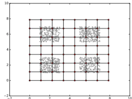
2 0 2 4 6 8 10 2 0 2 4 6 8

Fig. 3: Neuron’s weights linked through synapses

with values from (0,0) to (8,8). The graph in figure3illustrates such initial network, weights are represented by the position of nodes, and lateral synapses by the links between these nodes. Parameters like learning rate and elasticity have been fixed to α = 0.2 and η = 0.6 while pruning rate ω has been modified in order to analyze the effects of pruning.

The performance is measured by the average quantization error (AQE)4_{. This error represents the loss of information}

induced by the vector quantization on the overall vector sampling. It is usually computed as the mean quadratic error:

AQE = 1 p p X k=1 min 1≤i≤N(dist(vk, wi)) 2 ₍₄₎

Where p is a number of input vectors used as reference for computing the AQE, vk is one of the p vectors to be used for

computing the AQE, and N is the total number of neurons. dist(vk, wi) is the distance between the weight of neuron i and

the input vector vk. Only the minimum distance is considered

for AQE computation because this is the prototype vector representing the incoming data. p can be the complete vector training set or a subset of it. Using a subset is mandatory when the number of input vectors not known in advance or when the system runs online. In the experiments presented here, p has been fixed to 500.

Two different experiments have been carried out on these functions. The first one analyzes the effect of pruning on the worst case scenario (the third density function), and how AQE behaves under different pruning conditions. The second experiment aims to analyze the behavior of the best network of the first experiment when applied to two other probability functions.

2) The effect of pruning: The first experiment aims to observe how a network evolves under different values of ω. Figure 4 illustrates the behavior of PCSOM with 8 different values of ω applied on the third density function of figure2. Each curve in the figure represents the average of 48 runs of the algorithm with the same parameters. In this figure it can be observed the evolution of the network in terms of the total

4_{Another error measure for self-organizing maps is often used, the}

dis-tortionmeasure. For each input, a gaussian-weighted average of quantization errors is computed around the best matching unit. The distortion is the average over all inputs of all these computed weighted averages. This error measure reflects how much neighbouring neurons have learned similar prototypes. Since our model modifies the underlying topology, this error measure can not be satisfactorily applied to compare the performance of SOMs and PCSOMs.

0 5000 10000 15000 20000

iterations

0 20 40 60 80 100 120

number of synapses

ω =1e-07 ω =3e-07 ω =1e-06 ω =3e-06 ω =1e-05 ω =0 ω =3e-08 ω =3e-05

Fig. 4: Number of synapses vs. time for different pruning rates

0 5000 10000 15000 20000

iterations

0.05 0.06 0.07 0.08 0.09 0.10

AQE

ω=1e-07 ω=3e-07 ω=1e-06 ω=3e-06 ω=1e-05 ω=0 ω=3e-08 ω=3e-05

Fig. 5: AQE vs. time for different pruning rates

0 1 2 3 4 5 6 7 8 0 1 2 3 4 5 6 7 8

Fig. 6: Probability density function and weights after training the network with ω = 0

number of synapses over time. Figure 5 illustrates the AQE measured during the network’s lifetime. The color code of the two figures corresponds to the same evaluated pruning rates.

It can be observed that when ω = 0, meaning that no pruning is performed, the number of synapses remains constant at 112. It can also be observed that with ω = 0 the AQE converges quickly to a suboptimal value. Figure 6 illustrates a typical resulting network when pruning is disabled (ω = 0). It can be observed that learning has optimized the AQE by fitting the probability function. However, the network elasticity (the influence of lateral neurons) has prevented the network to correctly fit the function. Of course, a solution could be to reduce the elasticity, reducing in this manner lateral neuron influence. However, this solution would have other undesirable side effects like slowing down learning.

We observe in the other extreme case, with ω = 3e − 05, a network with a very high probability of pruning synapses. It results in a network that gets unconnected very quickly, and has not enough time to take advantage of the elasticity mechanism proposed by the algorithm and the measured AQE converges quickly to a very poor value. This is an extreme case of over-pruning. Another case of overpruning is with (ω =

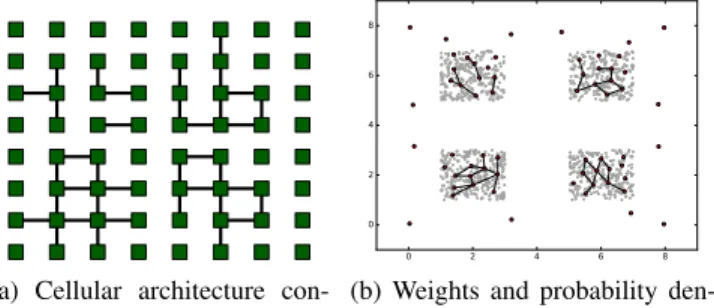
(a) Cellular architecture con-nections 0 2 4 6 8 0 2 4 6 8

(b) Weights and probability den-sity functions

Fig. 7: Results after training with ω = 1e − 05

(a) Cellular architecture con-nections 0 1 2 3 4 5 6 7 8 0 1 2 3 4 5 6 7 8

(b) Weights and probability den-sity functions

Fig. 8: Results after training with ω = 3e − 07

1e−05) the network is unable to converge to a stable structure and the over-pruning ends up eventually by disconnecting the whole network. Figure7bshows a network suffering of over-pruning. The very early synapse removal makes the network converge to a sub-optimal solution. Elasticity becomes useless and lateral influence is not present anymore.

The best solution is obtained with ω = 3e−07. The number of neurons converges to the optimal value achieving the best possible AQE for this probability function. It can also be observed that networks tested with the values ω = 3e − 08 and ω = 1e − 07 converge to almost the same number of neurons and almost the same AQE, the final result is thus as good as the best solution; however, they require a much higher number of iterations, making the learning unnecessarily slower.

An example of a resulting network using the pruning rate achieving the best performance can be observed in Figure8b. In this network the useless synapses highlighted in figure 6

have been removed, and only useful connections are main-tained. The formed sub-network naturally represents the four data clusters on the input data-set. Other pruning rate values like ω = 1e − 06 and ω = 3e − 06 converge to sub-optimal AQE values. In spite of the over-pruning, the network manages to stabilize its structure. However, given early synapse removal it is impossible to achieve the best performance.

In conclusion, the pruning mechanism is able to reduce AQE when used with the correct pruning rate parameter. If the pruning rate results to be smaller than the optimal value, it still converges to an optimal solution but learning is slower. On the other hand, if the pruning rate is higher, the network will fail to converge to the optimal solution. Excessive removal of synapses reduces the influence of a neuron on other neurons and reduces the capability of the SOM to work as a collaborative network. The other extreme

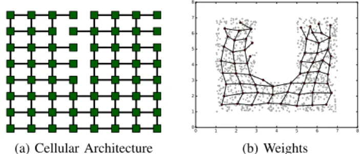
-(a) Cellular Architecture 0 1 2 3 4 5 6 7 8 0 1 2 3 4 5 6 7 (b) Weights

Fig. 9: Resulting neural network with the 1st probability density function 0 5000 10000 15000 20000 iterations 0 20 40 60 80 100 120 number of synapses ω =0 ω =3e-07 ω =1e-05

(a) Number of synapses

0 5000 10000 15000 20000 iterations 0.10 0.11 0.12 0.13 0.14 0.15 0.16 0.17 AQE ω=0 ω=3e-07 ω=1e-05

(b) Average quantization error Fig. 10: Network evolution for the 1st _{Probability Density}

Function (PDF) and Average Quantization Error (AQE)

without pruning - will maintain the original network with even useless connections, that may prevent the network to converge to optimal solutions.

3) Validating on other probability density functions: In order to validate the robustness of our approach, we have tested the same network with the same parameters on different probability density functions. We kept thus the same param-eters described in the previous subsection and we only used three different values for the pruning rate: the optimal value of ω = 3e − 07, a case of over-pruning with ω = 1e − 05, and without pruning ω = 0, in order to compare their performance. Only the resulting networks with ω = 3e − 07 are represented in figures9 and11.

Figure 9b shows that almost no pruning is performed in this function. Pruning does not contribute to minimize AQE and the network dynamics is able to adapt to the function characteristics. Nevertheless, given the stochastic nature of the pruning mechanism, it can still be possible to prune a connection (bottom right neuron in the figure), without negative consequences in this particular case.

Figure10illustrates the evolution of the network with three different values for ω over 20000 iterations. The graph repre-sents the average of 48 runs of the algorithm. From figure10b

it can be observed that the same parameter ω = 3e − 07 found in the first experiment as the optimal value, achieves the same quantization error than the network without pruning. It can also be observed that the network with very high pruning exhibits a poor performance. From figure 10ait can be observed that the over-pruning is even worse than the one observed in the previous experiment (figure4), and that the pruning performed on the network with ω = 3e − 07 is negligible.

It is worth to comment the effect observed around to itera-tion 1000 of figure 10b. After achieving a good quantization error, the network isn’t able to maintain it. This is due to the elasticity of the network regulated in equation 2 with the parameter η. This parameter regulates the influence of the

(a) Cellular Architecture

0 1 2 3 4 5 6 7 8 0 1 2 3 4 5 6 7 (b) Weights Fig. 11: Resulting neural network with the 2nd _PDF

0 5000 10000 15000 20000 iterations 0 20 40 60 80 100 120 number of synapses ω =0 ω =3e-07 ω =1e-05

(a) Number of synapses

0 5000 10000 15000 20000 iterations 0.08 0.09 0.10 0.11 0.12 0.13 0.14 AQE ω =0 ω =3e-07 ω =1e-05

(b) Average quantization error Fig. 12: Network evolution for the 2nd _PDF

weight of lateral neurons on the computation of each neuron weight. A high value of η makes it possible to converge faster, but may prevent the network to find an optimal solution at long term (like in this case). A solution may be to decrease over time the value of η in a similar way than SOM. However, doing so reduces the further network capability to adapt to different input data, making the algorithm unsuitable for learning dynamic functions.

Figure11shows the result of a network with ω = 3e − 07 and the same parameters, learning the 2nd_{probability density}

function of figure2, which still can benefit from the pruning mechanism. From a qualitative point of view, this figure permits to deduce that pruning has contributed to obtain a good solution. For a quantitative assessment, figure 12shows the behavior of PCSOM for 3 values of ω over 20000 iterations (each being the average of 48 runs). Again it can be observed that the network with a correct pruning parameter value achieves a better performance than the ones without pruning and with over-pruning.

From these two new probability density functions it can be observed that parameters are rather independent of the function at hand. The same set of parameters can be applied without knowing the function in advance.

B. Application to image compression

A well-known application of self-organizing maps is lossy image compression [24]. The principle is to divide the image into small sub-images, learn a good quantization of these sub-images, and then replace each sub-image by the index of the closest prototype. Uncompressing the image is then performed by replacing each index by the corresponding sub-image prototype. Compared to other quantization techniques, SOMs preserve topological properties, so that close parts of an image that are often similar will be coded by neighbouring neurons. It makes it possible to further reduce the size of the compressed file by efficiently coding prototype indexes [25].

In order to evaluate how PCSOM behaves in real-world ap-plications, we have decided to choose this image compression method as an example, performing the following steps:

1) The L × H picture is cut into I sub-images of l × h pixels, thus I = (L/l) × (H/h).

2) A SOM and a PCSOM of n × n neurons learn these sub-images. Each neuron has a l × h weight vector, that can be interpreted as a sub-image prototype.

3) The compressed image starts with the size of the original image, the size of the sub-images and the number of neurons. Then it includes a palette of the n × n sub-image prototypes, as learned by the SOM or PCSOM. Then, the compressed image only contains a list of the indexes of the winning neurons for each sub-image. Even without further compression of the index list thanks to topological properties of self-organizing maps, the compres-sion ratio for a grayscale image (1 byte per pixel) is thus:

L × H

20 + (n × n × l × h) + (L_l ×H

h × b)

where b is the minimal number of bits to code integers between 0 and n × n − 1.

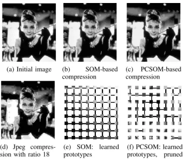
As an example, we consider a 364 × 332 image subdivided into 7553 sub-images of 4 × 4 pixels. Using a 8 × 8 SOM or PCSOM (b = 6), the compression ratio reaches a very high value of 18 (again, without the further compression of the index list using differential and entropy coding [25]). Based on 213experiments using various sets of parameters, PCSOM significantly improves the AQE (average 3.277e-2, standard deviation 3.16e-4) with respect to standard SOMs (average 3.464e-2, standard deviation 1.49e-3). We also observe a significant perceptual improvement of the visual result that is partially illustrated by the usual peak signal-to-noise ratio (PSNR) to be maximized: average 24.79 for PCSOM vs 23.54 for SOM. Figure 13shows results obtained for 20 epochs of 7553 iterations, each one using the same pattern for SOM and PCSOM learning though the ordering is random. Pruning is performed after each epoch. The compression examples correspond to the SOM or PCSOM that reaches the best PSNR. For this PCSOM, ω = 8.10−9, resulting in 51 pruned synapses. Most topological properties are maintained since this pruning occurs progressively during learning. It must be mentioned that PCSOM learning is very fast compared to SOMS, often reaching the SOM final performance after less than 10 epochs. Further studies need to be carried out to analyze the precise effect of pruning in this application.

An important amount of work still needs to be carried out so as to study how the induced self-organization of the computing resources may take advantage of the properties of PCSOM. In the specific case of this application to lossy image compression, it lies in the way prototype indexes asso-ciated to sub-images are further compressed. Following [25], a differential coding is first performed, computing differences between the index associated to a sub-image and the index associated to the neighbouring sub-image in the best local minimum gradient direction. Then these index differences are sent to an universal entropy coder using variable length

(a) Initial image (b) SOM-based compression

(c) PCSOM-based compression

(d) Jpeg compres-sion with ratio 18

(e) SOM: learned prototypes

(f) PCSOM: learned prototypes, pruned synapses

Fig. 13: SOM vs PCSOM for lossy image compression

coding. Thanks to the topological preservation property of self-organizing maps, the differential coding step mostly results in small numbers for which entropic encoding is very compact. Uncompression uses similar steps in a reverse order. In a parallelized version of the whole process, computing resources that will handle differential coding will have to communi-cate with other computing resources so as to compute index differences and local minimum gradient directions between ”winners” of neighbouring sub-images. When handling several sub-images in parallel, these communications will compete for NoC resources. The self-organization of computing resources with respect to PCSOM will minimize traffic congestion in the NoC, since the nodes that will often communicate will be very close according to the NoC constraints. Details of this work still need to be specified.

VI. CONCLUSION AND FURTHER WORK

In this paper we have presented the SOMA architecture, a neural-based processing architecture inspired by brain plastic-ity to tackle hardware self-organization of massively parallel processing elements. The bio-inspired process proposed by SOMA relies on an efficient learning of incoming data in order to dynamically adapt the size of processing areas to stimulation coming from the external environment. The learning process relies on a new neural model inspired by self-organizing maps. It has been adapted for cellular architectures and integrates pruning capabilities: it removes useless lateral connections in order to better fit the target probability density functions. The results of our experiments show that the proposed pruning mechanisms may improve the network performance by reduc-ing the average quantization error. We have also analyzed the effect of different values for the pruning parameter: very high values fail to achieve optimal AQE due to over-pruning, very low values converge to optimal solutions, but may be very slow.

PCSOM has been designed taking into account the con-straints imposed by the SOMA architecture, a cellular array of processing elements with dynamic routing and enhanced reconfigurability capabilities. Future works will implement PCSOM on this cellular architecture in order to drive the type of hardware to be configured on each node.

Further work will focus on analyzing the behavior of PCSOM on dynamic environments (i.e. probability density functions that change over time) and on studying the interest of including sprouting mechanisms in order to rebuild synapses or create connections with remote neurons. Again, dynamic routing of the underlying NoC architecture should permit this by still imposing physical constraints due to congestion probability.

ACKNOWLEDGMENT

The authors would like to thank the Swiss National Science Foundation (SNSF) and the French National Agency (ANR) for funding the SOMA project (ANR-17-CE24-0036).

REFERENCES

[1] A. SATURN, “The saturn project - self-adaptive technologies for up-graded reconfigurable neural computing, french research agency (anr), http://projet-saturn.ensea.fr,” 2011-2014.

[2] C. R. Rupp, M. Landguth, T. Garverick, E. Gomersall, H. Holt, J. M. Arnold, and M. Gokhale, “The napa adaptive processing architecture,” in Symp. on FPGAs for Custom Computing Machines, 1998, pp. 28–37. [3] M. Wazlowski, L. Agarwal, T. Lee, A. Smith, E. Lam, P. Athanas, H. Silverman, and S. Ghosh, “Prism-ii compiler and architecture,” in FPGAs for Custom Computing Machines, 1993. Proceedings. IEEE Workshop on. IEEE, 1993, pp. 9–16.

[4] P. M. Athanas and H. F. Silverman, “An adaptive hardware machine architecture and compiler for dynamic processor reconfiguration,” in Computer Design: VLSI in Computers and Processors. ICCD’91. Pro-ceedings, IEEE International Conference on. IEEE, 1991, pp. 397–400. [5] D. Mange, M. Sipper, A. Stauffer, and G. Tempesti, “Toward robust integrated circuits: The embryonics approach,” Proceedings of the IEEE, vol. 88, no. 4, pp. 516–540, April 2000.

[6] Y. Thoma, G. Tempesti, E. Sanchez, and J. M. M. Arostegui, “POEtic: an electronic tissue for bio-inspired cellular applications,” Biosystems, vol. 76, no. 1-3, pp. 191–200, 2004.

[7] E. Sanchez, A. Perez-Uribe, A. Upegui, Y. Thoma, J. M. Moreno, A. Napieralski, A. Villa, G. Sassatelli, H. Volken, and E. Lavarec, “Per-plexus: Pervasive computing framework for modeling complex virtually-unbounded systems,” in Adaptive Hardware and Systems (AHS). Second NASA/ESA Conference on. IEEE, 2007, pp. 587–591.

[8] J. B. Macqueen, “Some methods of classification and analysis of mul-tivariate observations,” in Proceedings of the Fifth Berkeley Symposium on Mathematical Statistics and Probability, 1967, pp. 281–297. [9] A. B. Y. Linde and R. Gray, “An algorithm for vector quantization

design,” IEEE Trans. on Communications, 1980.

[10] T. Kohonen, “Self-organized formation of topologically correct feature maps,” Biological Cybernetics, vol. 43, 1982.

[11] T. M. Martinetz, S. G. Berkovich, and K. J. Schulten, “Neural-gas network for vector quantization and its application to time-series pre-diction,” IEEE Trans. on Neural Networks, vol. 4, no. 4, 1993. [12] B. Fritzke, “A growing neural gas network learns topologies,” in

Advances in Neural Information Processing Systems 7, G. Tesauro, D. Touretzky, and T. Leen, Eds. MIT Press, 1995, pp. 625–632. [13] K. S., J. Jangas, and T. Kohonen, “Bibliography of self-organizing map

papers: 1981-1997,” Neural Computing Surveys, 1998.

[14] O. M., K. S., , and T. Kohonen, “Bibliography of self-organizing map papers: 1998-2001 addendum,” Neural Computing Surveys, 2003. [15] J. Misra and I. Saha, “Artificial neural networks in hardware: A survey

of two decades of progress,” Neurocomputing, vol. 74, no. 1–3, pp. 239 – 255, 2010, artificial Brains.

[16] W. Kurdthongmee, “A hardware centric algorithm for the best matching unit searching stage of the som-based quantizer and its fpga implemen-tation,” Journal of Real-Time Image Processing, vol. 12, no. 1, 2016.

[17] M. A. de Abreu de Sousa and E. Del-Moral-Hernandez, “Comparison of three FPGA architectures for embedded multidimensional categorization through Kohonen’s self-organizing maps,” in 2017 IEEE International Symposium on Circuits and Systems (ISCAS), May 2017, pp. 1–4. [18] N. P. Rougier and Y. Boniface, “Dynamic Self-Organising Map,”

Neu-rocomputing, vol. 74, no. 11, pp. 1840–1847, 2011.

[19] L. Rodriguez, B. Miramond, and B. Granado, “Toward a sparse self-organizing map for neuromorphic architectures,” ACM Journal on Emerging Technologies in Computing Systems, vol. 11, no. 4, 2015. [20] L. Rodriguez, L. Fiack, and B. Miramond, “A neural model for hardware

plasticity in artificial vision systems,” in Proceedings of the Conference on Design and Architectures for Signal and Image Processing, 2013. [21] L. Fiack, B. Miramond, A. Upegui, and F. Vannel, “Dynamic parallel

reconfiguration for self-adaptive hardware architectures,” in NASA/ESA Conference on Adaptive Hardware and Systems (AHS-2014), 2014. [22] F. Moraes, N. Calazans, A. Mello, L. M¨oller, and L. Ost, “Hermes: an

infrastructure for low area overhead packet-switching networks on chip,” INTEGRATION, the VLSI journal, vol. 38, no. 1, pp. 69–93, 2004. [23] L. Khacef, B. Girau, N. P. Rougier, A. Upegui, and B. Miramond,

“Neuromorphic hardware as a self-organizing computing system,” in WCCI 2018 - IEEE World Congress on Computational Intelligence, Workshop NHPU : Neuromorphic Hardware In Practice and Use, IEEE, Ed., Jul. 2018, pp. 1–4.

[24] Z. Huang, X. Zhang, L. Chen, Y. Zhu, F. An, H. Wang, and S. Feng, “A hardware-efficient vector quantizer based on self-organizing map for high-speed image compression,” Applied Sciences, vol. 7, no. 11, 2017. [25] C. Amerijckx, J. Legat, and M. Verleysen, “Image compression using self-organizing maps,” Systems Analysis Modelling Simulation, 2003.