Budding yeast cell cycle analysis and morphological characterization by automated image analysis

Budding Yeast Cell Cycle Analysis and Morphological

Characterization by Automated Image Analysis

by

Elizabeth Perley

B.Sc., Massachusetts Institute of Technology, 2010

Submitted to the Department of Electrical Engineering and Computer Science in Partial Fulfillment of the Requirements for the Degree of

Master of Engineering in Electrical Engineering and Computer Science at the

Massachusetts Institute of Technology May 2011

[3unt -2C

@2011

Massachusetts Institute of Technology All rights reserved.

MASSACHUSETVS INSTTUTE OF TECHL.O' y

JUN

2 1 2011

L IBRA R IES

ARCHIVES

The author hereby grants to M.I.T. permission to reproduce and to

distribute publicly paper and electronic copies of this thesis document in whole and in part in any medium now known or hereafter created.

A u th or ... ... . . . ... Department of Electrical Engineering and Computer Science

May 20, 2011

C ertified .by ...

Mark Bathe, Assistant Professor Thesis Supervisor

A ccepted by ... .. ...

Dr. Christopher J. Terman Chairman, Masters of Engineering Thesis Committee

Budding Yeast Cell Cycle Analysis and Morphological

Characterization by Automated Image Analysis

by

Elizabeth Perley

Submitted to the Department of Electrical Engineering and Computer Science in partial fulfillment of the requirements for the degree of

Master of Engineering

Abstract

Budding yeast Saccharomyces cerevisiae is a standard model system for analyzing cellular response as it is related to the cell cycle. The analysis of yeast cell cycle is typically done visually or by using flow cytometry. The first of these methods is slow, while the second offers a limited amount of information about the cell's state. This thesis develops methods for automatically analyzing yeast cell morphology and yeast cell cycle using high content screening with a high-capacity automated imaging system. The images obtained using this method can also provide information about fluorescently labelled proteins, unlike flow cytom-etry, which can only measure overall fluorescent intensity. The information about yeast cell cycle stage and protein amount and localization can then be connected in order to develop a model of yeast cellular response to DNA damage.

Thesis supervisor: Mark Bathe Supervisor title: Assistant Professor

Abstract

Table of Contents List of Figures List of Tables 1 Introduction

2 Related work and Background

2.1 Background . . . . 2.1.1 Yeast cell cycle stage and response to DNA damage . . . . 2.1.2 Yeast Cell Cycle Analysis and Morphological Characterization by

Mul-tispectral Imaging Flow Cytometry . . . . 2.2 Current cell detection and classification software . . . . 2.2.1 C ellProfiler . . . .

3 Overview

4 Image Processing

4.1 Im aging . . . . 4.1.1 Bright field images vs. Concanavalin A images . . . . 4.2 Cell detection and segmentation . . . . 4.2.1 Edge detection with watershedding of bright field images . 4.2.2 Thresholding using Concanavalin A . . . . 4.2.3 Voronoi-based segmentation using CellProfiler . . . . 4.2.4 Yeast-specific cell detection and segmentation . . . . 4.3 Nucleus detection and segmentation . . . . 4.4 Discussion . . . .. . . . . . . - .

Cycle Stage Classification

Creation of a training set . . . . Feature selection . . . .

Table of Contents

2 3 5 6 7 10 10 10 11 13 13 15 16 . . . . 16 . . . . 16 . . . . 18 . . . . 19 . . . . 23 . . . . 25 . . . . 27 . . . . 31 - - - 33 34 35 36 5 Cell 5.1 5.2

5.3 Feature calculation . . . . 5.3.1 Basic cell features . . . . 5.3.2 Bud detection . . . . 5.4 Feature validation . . . . 5.4.1 Using the training set . . . . 5.4.2 Using cells arrested in stages of cell cycle 5.5 Classification using neural nets . . . . 5.5.1 Creation of the neural net . . . . 5.5.2 Net performance on training set . . . . . 5.5.3 Net performance on additional data . . .

6 Conclusions 7 Appendices

7.A Edge detection and watershedding code . . . . 7.B Concanavalin A thresholding code . . . . 7.C Nucleus detection code . . . . 7.D Feature calculation code . . . . 7.E Bud detection code . . . . References . . . . 3 7 . . . . 3 8 . . . . 3 8 . . . . 4 2 . . . . 4 2 . . . . 47 . . . . 5 1 . . . . 5 1 . . . . 5 2 . . . . 5 2 58 60 60 62 63 64 65 70

1 2 3 4 5 6 7 8 9 10 11 12 13 14 15 16 17 18 19 20 21 22 23 24 25

Bright field image of budding yeast cells . . . . Bright field image of budding yeast cells . . . . Comparison of bright field and ConA images . . . . Edge detection and watershedding to segment cells... Distance transform of cells . . . . Edge detection and watershedding on ConA images... CellProfiler Cell Segmentation . . . . Polar plot of yeast cells for segmentation . . . . Yeast-specific cell detection algorithm to detect cells . . . . . Budding yeast cell cycle stages. Adapted from Calvert, et al. Cell undergoing bud detection algorithm . . . ... . .. Cell area feature distribution. . . . . Average nuclear intensity distributions. . . . . Overall nuclear intensity distributions. . . . . Bud size distributions . . . . Bud/mother cell ratio distributions. . . . . Cell area - Arrested Cells vs. Training set Comparison. . . .

Average nuclear intensity - Arrested Cells vs. Training set Comparison Bud size - Arrested Cells vs. Training set Comparison . . . . Neural net used for classification . . . . Cell area feature distribution. . . . . Average nuclear intensity distributions. . . . . Overall nuclear intensity distributions. . . . . Bud size distributions . . . . Bud/mother cell ratio distributions. . . . .

List of Figures

8 . . . . 15 . . . . 18 . . . . 2 1 . . . . 2 2 . . . . 23 . . . . 2 6 . . . . 29 . . . . 30 ] . . . . 34 . . . . 40 . . . . 44 . . . . 4 5 . . . . 4 6 [2 50 51 52 54 55 55 56 56

List of Tables

1 Feature list for classification . . . . 36

2 Differentiation between G1 and G2 using a feature subset . . . . 37

3 Differentiation between G1, S and G2/M using a feature subset . . . . 38

4 Estimated cell diameter . . . . 44

5 Neural net performance on training set . . . . 53

6 Neural net performance on all data . . . . 53

7 Estimated cell diameter . . . . 54

1

Introduction

In recent years there has been a significant amount of development in the area of high content (HC) imaging. This technique attempts to combine high throughput with high resolution imaging to provide statistics with a large number of samples, and images which provide accurate measurements. A number of platforms and a several pieces of software are now available to acquire and analyze images from HC screens. However, most of these were developed specifically for mammalian cells, which are large and grow in single layers, and therefore make assumptions about the types of images that can be used as input lack the ability to deal with other types of cells.

One type of cell that these platforms are often not capable of dealing with is the budding yeast (Saccharomyces cerevisiae) cell. Budding yeast cells are one of the standard model systems in biology. Their cell-cycle has been well characterized in terms of cellular morphol-ogy as well as in the proteins involved, and there is a large amount of biological knowledge that exists. This makes them an excellent choice for developing models. However, these cells do not grow in a single layer, and they are quite small compared to mammalian cells, so in order to use HC imaging, a new tool for analysis must be used.

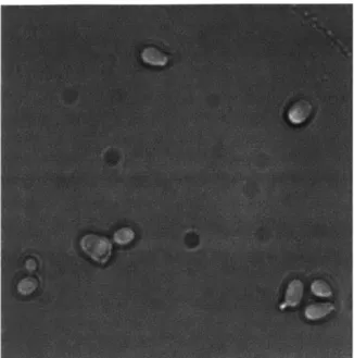
The first part of this thesis describes methods to analyze HC images of budding yeast cells. First, cell outlines must be determined from the images of cells. Each well on a plate contains hundreds of cells and requires multiple images to be taken, each of which contains tens of cells. These cells must be correctly identified, and accurately segmented and outlined to get the correct cell shape, as well as to allow for the correct calculation of protein levels and localization. This problem poses several challenges: The images are taken automatically, and as a result are not always completely focused. They also often have uneven illumination, and contain other particles or out of focus cells, which contribute to noise and misidentification of cells. Budding yeast cells also have very thick cell walls, making the decision to find the

Figure 1: Bright field image of budding yeast cells

"correct" cell border a difficult one. This can be seen in Figure 1. It is unclear if it is at the outer cell border, or the inner cell border, or somewhere in between. Several different approaches for cell segmentation were investigated, and the best selected.

The second part of this thesis describes a way to use these image analysis methods to develop a model of how budding yeast cells respond to DNA damage. When a cell's DNA becomes damaged, the cell must respond in some way in order to repair its DNA and continue its progress in the cell cycle. Many genes and pathways have been found that are responsive to DNA damage in budding yeast, using techniques such as bulk transcriptional profiling and genomic phenotyping assays. However, little is known about the mechanism by which these changes occur, and how protein levels and localization with in the cell are affected by damage.

Previously, flow cytometry was used to study this response. However, this method only allows overall protein and DNA levels to be measured. It has been shown that the response of budding yeast cells is dependent on their current stage of the cell cycle, which cannot be seen using flow cytometry. Although it is possible to arrest cells at specific stages of the cell

cycle with drugs, these may introduce artifacts. Since HC imaging allows cell morphology to be examined and cell cycle determined, this approach offers a significant advantage and it can provide a more detailed picture of the response of budding yeast.

The paper describes a machine learning approach to classifying yeast cells into their cell cycle stages. Once the cell cycle stages can be accurately identified from cell shape and nuclear shape, DNA content and position, then asynchronous populations of yeast cells can be characterized. Algorithms to find the bud of a cell and calculate morphological features of the cells were developed. Using these features, neural nets were tested as ways to classify these cells in a supervised learning approach.

2

Related work and Background

2.1

Background

2.1.1 Yeast cell cycle stage and response to DNA damage

Previous work has been done to determine the cellular response of budding yeast to DNA damaging agents by Jelinsky, et al.[10] In their paper, budding yeast cells were exposed to various carcinogenic alkylating agents and oxidizing agents, as well as ionizing radiation, and it was found that this exposure modulates transcript levels for over one third of the genes of the yeast cells. What was particularly relevant about these results was the finding that for one of the carcinogenic agents, MMS, the response is dramatically affected by the cell's position in the cell cycle at the time that it is exposed to the agent.

Cultures of log-phase budding yeast cells were arrested in G1 by a-factor, in S phase by hydroxyurea, and in G2 by nocodazole. These cells were then allowed to grow for three days before each group of cells was split in half and MMS added to one of the two halves in each phase.

In order to investigate the cellular response to the addition of MMS, GeneChip hybridiza-tions were used. A set of arrays was used contianing probes for 6,218 yeast ORFs and then analyzed using the GeneChip analysis suite. Then, any gene which showed a change of 3.0-fold or more in at least one of the experimental conditions was further examined. The result was that there were 693 such genes which were responsive to treatment with MMS. These were shown to be certainly responsive, with none of the error bars for treated and untreated cells coming close to overlapping.

Initially, when asynchronous log-phase cultures were treated with MMS, many genes were scored only as weakly responsive. However, treating yeast cells which had been arrested in

the stages of the cell cycle caused many more genes to be shown as clearly responsive to the treatment. Of the genes that were responsive, 199 were responsive only in G1, 84 were

responsive only in S phase, 94 were responsive only in G2, and 229 were responsive only in

stationary phase. Prior to these experiments, fewer than 20% of the genes examined had been shown to have cell-cycle dependent expression.

These results indicate that, in order to fully understand the budding yeast response to damage, each cell's stage in the cell cycle must be taken into account.

2.1.2 Yeast Cell Cycle Analysis and Morphological Characterization by Multi-spectral Imaging Flow Cytometry

Yeast cell cycle analysis has previously been done using multispectral imaging flow cytometry (MIFC) in a computational approach. [2] In a paper by Calvert, et al., an improvement on the traditional yeast cell cycle analysis using flow cytometry is developed. MIFC offers multiple parameters for morphological analysis, allowing for the calculation of a novel feature, bud length, which is used to observe the change in morphological phenotypes between wild-type yeast cells, and those which overexpress NAP1, which causes an elongated bud phenotype.

An imaging flow cytometer was used, which allows the simultaneous detection of bright field, dark field, and four fluorescent channels. The images from MIFC were then used to visually assign cells to one of the three stages of the cell cycle: G1, S, and G2/M. They were

distinguished as cells in G1 being those that have a single nucleus and no bud, S being cells

with a single nucleus and a visible bud, and G2/M being those with elongated or divided

nuclei and a large bud.

The yeast cell cycle was determined using a combination of DNA intensity and nuclear morphology. Cells were split into ones that contained IN DNA content and round nuclei, 2N DNA content and round nuclei, and 2N DNA content and elongated or divided nuclei,

and these three groups were labelled as G1, S, and G2, respectively. 100 cells from each stage

of the cell cycle were then visually identified and labelled in order to validate this method of determining cell cycle, which was 99% accurate. Further testing of this method of cell cycle analysis was performed, and results from visual analysis of morphology and from this method of separation were similar, and far more accurate that analysis with standard flow cytometry using a cell cycle modelling program.

The bright field images were analyzed automatically to calculate the bud length feature. To do this, an object mask for the cell was calculated by separating the cell from its back-ground using pixel intensity in the bright field channel. This mask was then eroded by 3 pixels. Then, the bud length was calculated by subtracting the maximum thickness of the cell calculated from MIFC, which is assumed to be the diameter of the mother cell, from the total length of the cell as determined from the object mask. Relative bud length was calculated to be the ratio of the minimum thickness of the cell calculated from MIFC, and the width of the bud. The cell aspect ratio was calculated as the ratio between the total cell length and the width. Then, any cell which had a relative bud length larger than 1.5, and an aspect ratio of less than 0.5 was considered to be a cell with an elongated bud. The NAP1 strains and wild-type strains were then analyzed for differences in bud length as well as cellular shape. It was shown that MIFC could accurately distinguish between the elongated bud phenotype and a normal bud phenotype.

This approach shows that it is possible to determine cell cycle stage with MIFC using simple computational methods. In this case, a simple scatter plot was used to separate the cells between G1, S and G2, using DNA content and nuclear morphology. It also shows that

2.2

Current cell detection and classification software

2.2.1 CellProfiler

CellProfiler aims to perform automatic cell image analysis for a variety of phenotypes of cells from different organisms.

[4]

It is useful for measuring a number of cell features, including cell count, cell size, cell cycle distribution, organelle number and size, cell shape, cell texture, and the levels and localization of proteins and phosphoproteins. The motivation behind the creation of CellProfiler is to provide quantitative image analysis, as opposed to human-scored image analysis, which is qualitative and usually classifies samples only as hits or misses. It also allows the processing of data at a much quicker rate, and the creators consider cell image analysis to be one of the greatest remaining challenges in screening.

The software system consists of many already- developed methods for many cell types and assays. It uses the concept of a pipeline of these individual modules, where each module processes the images in some manner, and the modules are placed in a sequential order. The standard order for this processing first contains image processing, then object identification, and finally measurement.

According to the developers of CellProfiler, the most challenging step in image analysis is object identification. It is also one of the most important steps, since the accuracy of object detection determines the accuracy of the resulting cell measurements. The standard approach to object identification in CellProfiler is to first identify primary objects, which are often nuclei identified from DNA-stained images. Once these primary objects have been identified, they are used to help identify and segment secondary objects, such as cells. The identification first of primary objects helps to distinguish between different secondary objects, since they are often clumped. In the software, first the clumped objects are recognized and separated, then the dividing lines between them are found. Some of these algorithms for object identification are discussed later in subsection 4.2. One of these was specifically

developed for CellProfiler, which was an improved Propagate algorithm and allowed cell segmentation for some phenotypes to be performed which had never been possible previously.

The main testing of CellProfiler was performed on Drosophila KC167 cells because they are particularly challenging to identify using automated image analysis. It was also tested on many different types of human cells, and has been shown to work well on mouse and rat cells as well.

One of the main goals of CellProfiler was to be able to identify a variety of phenotypes and to be flexible, modular, and to make setting up an analysis feasible for non-programmers. This means that it does not have many modules for specific cell types, but rather more general ones that are applicable to many different types, which does make it good for many applications. However, for specific applications, or for cell types that it wasn't designed for, CellProfiler is not always a good fit.

3

Overview

The approach to examine budding yeast cellular response to DNA damage is outlined in Figure 2. First, images of cells are acquired using a Cellomics high-content automated imaging system. They then undergo image processing, which involves cell detection and segmentation, as well as nucleus detection. As described in the CellProfiler approach, this step is the most important because it determines the accuracy of all other measurements.

Segment cells

_A

Segment nuclei

Measure features of cells (Size, intensity, bud size, etc)

Classify cells according to stage of cell cycle

Calculate statistical metrics to determine quality of features and classification

Figure 2: Bright field image of budding yeast cells

Once the cells have been detected, then features of these cells are measured, such as cell size, shape, and nuclear size, shape, and intensity. These features are then used as input to a supervised learning system in order to classify cells as being in one of the three cell-cycle stages: G1, S, or G2/M. Finally, the features and the classification system are validated and tested.

Once cell cycle can be accurately determined, it is possible to measure other features of the cell from fluorescent channels and combine these measurements with the cell cycle information to learn more about the yeast cell response to DNA damage.

4

Image Processing

4.1

Imaging

The yeast library which was used was developed at the University of California San Francisco, and is now commercially available. It consists of yeast strains in which individual proteins are expressed with C-terminal GFP tags from endogenous promoters. The cells were fixed and stained with DAPI for visualizing the DNA, and with Concanavalin A for visualizing the cell walls. These cells were then imaged on 96-well plates using a Cellomics system from Thermofisher Scientific. Images were acquired in three fluorescent channels (for DAPI, GFP, and Concanavalin A) and in the bright field channel to allow ready visualization of cell contours.

4.1.1 Bright field images vs. Concanavalin A images

The standard way of viewing cell morphology is through the use of bright field images. These images show the basic cell outline of the budding yeast cells. However, these bright field images might not provide the best data for a high content screening approach for the following reasons:

" It is difficult even for a human to determine what the actual boundary of the cell is due to the thickness of the cell wall in the bright field images

" Cell buds are difficult to see due to the thickness of the cell wall, especially when they are small.

* Bright field images show not only cells, but also other particles in the well, and out of focus cells, which must be removed for further analysis of the cell images

Despite these problems, bright field is a type of image worth exploring for looking at cells because it requires no additional stains or steps in cell preparation. It also doesn't require the use of a GFP channel on the Cellomics imaging platform, which only has a limited number of channels.

Another choice for viewing cell morphology is to use cells which have been stained with fluorescent-conjugated Concanavalin A (ConA). ConA is a lectin which combines with pro-teins on the budding yeast cell walls. ConA provides a much clearer image of yeast cell morphology for the following reasons:

" Cell outlines are well defined with no ambiguity " Even small buds can be easily seen

" There is a minimal amount of noise, with no extra particles or out-of-focus cells, due to the fact that this is a fluorescent image

However, this requires the use of an additional channel in the microscope, which is only capable of taking pictures in 4 channels. Although in this paper not all channels are needed, it is desirable to have additional channels available so that multiple molecules in the cell may be observed.

The other drawback to using ConA images is the fact that the definitions between cells isn't quite as clear. While it is quite easy to tell which parts of the images are cells and which aren't, it can be difficult to distinguish between different cells in a cluster. This is due to the fact that there is no actual outline of the cell, and the entire cell is stained with ConA. However, use of a more dilute sample can alleviate this problem.

In subsubsection 4.1.1, the comparison between bright field and ConA images is clear. ConA images provide a much clearer view of the cells. Although some groups have had success with segmenting cells using bright field images alone

[13],

ConA images were chosen

Figure 3: Comparison of bright field (left) and ConA (right) images of budding yeast cells

after the investigation of the use of both types of images. Bud size is an easy way to roughly determine cell cycle stage, so the ability to calculate precise cell outlines was a major deciding factor in the choice of images . It is also important that the amount of protein in the cell can be determined. If the correct cell outlines are not found, then the amount of protein can be overestimated or underestimated.

4.2

Cell detection and segmentation

The cells in any image must first be separated from their background before further analysis can be done. While for many applications, only a cell count or a rough estimate of the cell shape and size is necessary, an accurate border is required in order to detect the bud and compute levels of fluorescence correctly.

4.2.1 Edge detection with watershedding of bright field images

There are three major challenges in detecting and segmenting cells. One of these is that the bright field images are the preferred choice for cell detection. However, the cell cannot simply be thresholded out in these images due to a low level of contrast between cells and the background. Another such challenge is the presence of non-cellular objects within the bright field images. Each object that is detected must be a cell, so any object that might be mistaken for a cell must be identified and removed. The last challenge is the fact that the cells are often grouped very closely together, and the cell detection algorithm must be able to separate these clusters.

Edge detection

One way to detect the cells in the low-contrast bright field images is to perform edge de-tection. Edge detection algorithms calculate the gradient across the image and then use a cutoff threshold to determine which values are a part of an edge, and which are not. This procedure uses the Canny edge detection algorithm.

[3]

This algorithm is designed to mark each edge only once, detect edges as close as possible to the actual edges in the image, and to not be affected by noise in the original image.

The cell detection algorithm is outlined as follows, and code be found in appendix 7.A:

1. Apply a Gaussian filter to reduce the amount of noise in the original image 2. Use the Canny algorithm to detect edges in the image.

3. Dilate the detected edges with linear elements. This fills in small gaps in the edges, which occur due to the fact that the image is very low-contrast, making it difficult to detect a full outline of each cell.

5. Erode with a circular element to smoothen the cells. 6. Remove objects that are too small to be cells.

Although the Canny edge detection algorithm has a noise removal step in it, the first step of the cell detection applies a Gaussian blur for further noise removal. This causes the edge detection to detect fewer incorrect small edges, since the cells are large enough such that this step does not affect their edges significantly. The MATLAB canny function can takes an argument that specifies the sensitivity threshold. In the code, a sensitivity value of 0.3 was chosen, which was also chosen to minimize the number of incorrect small edges while still detecting the main cell outlines.

Once edges have been detected, there are often gaps in the full cell outlines. These must be removed so that a cell mask can be created by filling in the outlines. Dilating the edges with a small horizontal and vertical linear element fills in the majority of these small gaps.

After the cells have been filled in, the cell mask which has been created is slightly larger than the cell. This is partially due to the fact that the edges were dilated, but also due to the fact that the cell wall is quite thick in the bright field images. For any particular cell, two edges are detected: the outside edge of the cell wall, and the inside edge of the cell wall. The cell border is actually somewhere in between these two lines, so the cell must be eroded a small amount. This erosion step can also help to smoothen the jagged edges that can be created due to the edge detection. A circular element is used for the erosion to maintain as much of the original cell shape as possible. The erosion also removes any objects which are too thin in one dimension to possibly be a cell.

Although the last erosion step is necessary, it removes quite a bit of detail from the cell outlines. While it smooths the jagged edges, it also can remove small buds from the cell. It also erodes the cell shape such that it is not always clear where the bud of the cell is exactly.

Figure 4: Using edge detection and watershedding to segment cells

Watershedding

After cell detection has been performed, the cells must still be segmented, since clusters of cells still remain. One standard algorithm which is used for cell segmentation is watershed-ding. [6] The basic concept behind watershedding is that the image is treated as a height field, and then the pixels are separated based on which minimum a drop of water would flow to if it were placed on that pixel in the height field.

In order to perform watershedding, first a distance transform is calculated on the cell mask obtained from the cell detection process. This involves calculating the distance from any pixel which is part of a cell to the closest pixel which is not part of a cell. So, pixels which are at the center of a cell have the highest values. An example of this can be seen in Figure 4.2.1. The values are then negated, and watershedding is performed. This means that any pixel which is considered to be part of a cell is assigned to the local minimum to which a drop of water would flow to if it were placed on that pixel in the negated distance transform. In Figure 4.2.1 these local minima would be the brightest pixels in the distance

Figure 5: Comparison of cell mask (left) with its distance transform (right)

transform.

However, watershedding is not an ideal method for cell segmentation. It can be practical because it is quick and can give a reasonable estimate of the number of cells in an image as well as the approximate area of the cells. However, a single noisy pixel can affect the grouping of an entire cluster of pixels by creating a gap between the group and a diferent minimum. The cell borders which are finally detected are also only somewhat related to the original image, meaning that when the cells in a cluster are segmented, the line chosen is based on the distance transform, rather than any edges that were present in the original image. Then, by the time the watershedding is performed, the cell outlines have already been manipulated so much that the distance transform is not a good measure of where the cells lie.

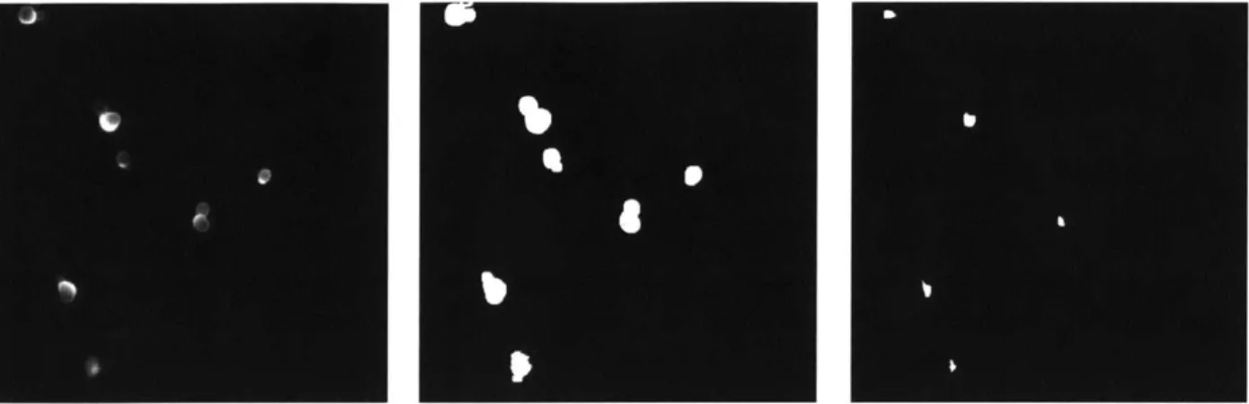
Even on images which are not noisy and segmentation should be easy, such as the ConA images, edge detection with watershedding does not perform well. This can be seen in Figure 6, where this same algorithm was run on ConA images of cells. Although the initial segmentation of the cells was trivial, the subsequent steps caused much of the clarity of the cell outlines and shapes to be lost, resulting in a final cell mask which has lost a great deal of information.

Figure 6: Comparison of original ConA image (left) with its cell outlines after edge detection (middle) with the final output after smoothing and watershedding (right)

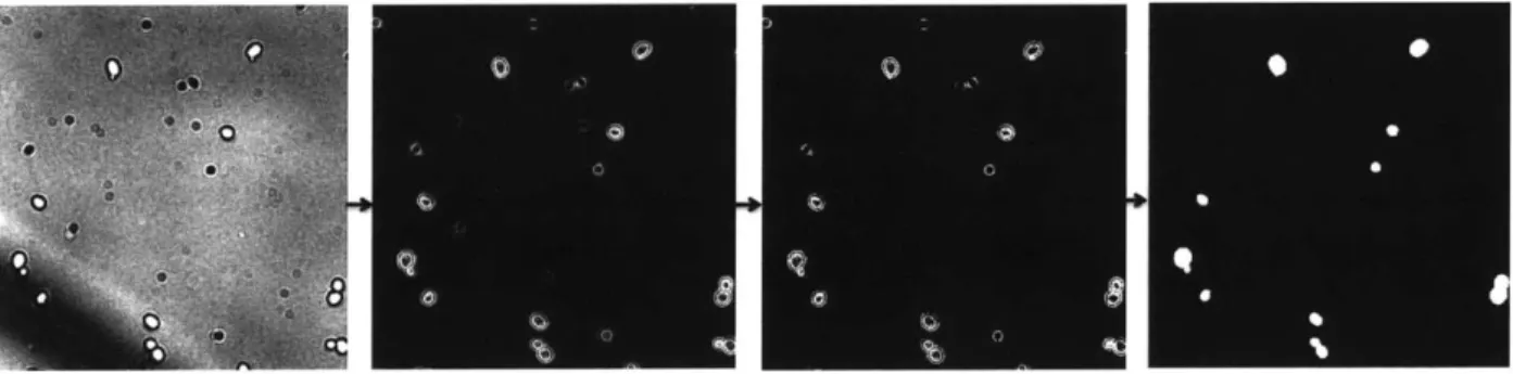
4.2.2 Thresholding using Concanavalin A

Images of yeast cells taken using Concanavalin A stain in a fluorescent channel provides a much better source image to work with than bright field images. The cell outlines are clear, and since the images are high-contrast, thresholding the cells from their background is possible. This makes cell detection a trivial task.

The cell detection algorithm is outlined below, and its code can be found in appendix 7.B:

1. Use a Gaussian filter to remove noise in the image

2. Adjust the contrast of the image so that the brightest pixels are as bright as possible and the darkest are as dark as possible. This helps to prepare the image so that it can be thresholded most easily.

3. Perform morphological closing on the image, to remove uneven brightness in the cells. [6] This occurs due to the fact that the edges of the cells appear brighter in the ConA images, since ConA is a cell wall stain. Morphological closing helps to remove gaps in the middle of the cell.

5. Fill in the interiors of the cells by filling in every closed outline in the image.

6. Fill in the gaps in any outlines of the cells using linear line elements, and then fill in any new holes created.

7. Remove objects which are too small or too large to be cells

The first step of the cell detection applies a Gaussian blur of size 3 x 3 for further noise removal. This smooths the cells to allow smooth cell borders to be detected once the image is thresholded. Then the values of the image are scaled such that they take on the full range of possible pixel values. Spreading the values out in this way allows the image to be thresholded more easily. The morphological closing is performed to fill in gaps in the middle of the cells and to even out some of the cell brightness. Though the interiors of the cells will be later filled in, this is done as a preventative measure to also ensure that there are not gaps at the edge of the cells which cannot get filled in.

This image is then turned into a black and white cell mask using an automatically calculated threshold value. The standard MATLAB greythresh method is used. This method implements Otsu's method, which chooses the threshold to minimize the intraclass variance of the black and white pixels. [16] This function is used to calculate a starting point for a cutoff threshold, and then this is scaled by a factor of 0.8 to adjust it for the image set being used. After the cells are filled in, there are still some remaining portions of cell outlines which have not been filled in. The image is dilated with small linear elements using many different angles to fill in the largest number of gaps possible. Any new cell interiors which have been created are then filled in using MATLAB's imf ill method, which fills in any background pixels which cannot be reached from the edge of the image.

However, cell segmentation still presents a problem. Watershedding loses information about cell shape as shown in the previous section. This problem can be dealt with by using a sample of cells which is dilute enough such that there are few clusters of cells, which are

then not included in further data analysis (they get removed in the last step of the cell detection algorithm). It also might be possible to segment these cells using an algorithm such as that described in the next sections. This problem ended up being beyond the scope of the thesis, but would be good for further investigation.

4.2.3 Voronoi-based segmentation using CellProfiler

The CellProfiler software discussed in subsubsection 2.2.1 uses a novel method of segmenting cells using Voronoi regions. [12] This approach was designed to overcome the limitations of watershedding that cause it to be a fragile algorithm for segmenting cells. It does so by comparing neighborhoods of pixels rather than individual pixels to avoid the issue of a single noisy pixel affecting the segmentation of a group of pixels. It also tries to segment cells based on the borders found in the original image but includes a regularization factor to provide reasonable behavior when there is not a strong edge between two cells.

Unlike the other algorithms which relied only on the image of the cell morphology to detect and segment cells, this approach relies on an image of the nuclei as well. It considers these nuclei to be seed regions, and proceeds to find a cell for each nucleus detected.

The CellProfiler platform provides an implementation of this algorithm, and the image of detected nuclei from subsection 4.3 was used to provide the seed regions for the algorithm. Both bright field and ConA images were used as potential source images for which to segment the cells.

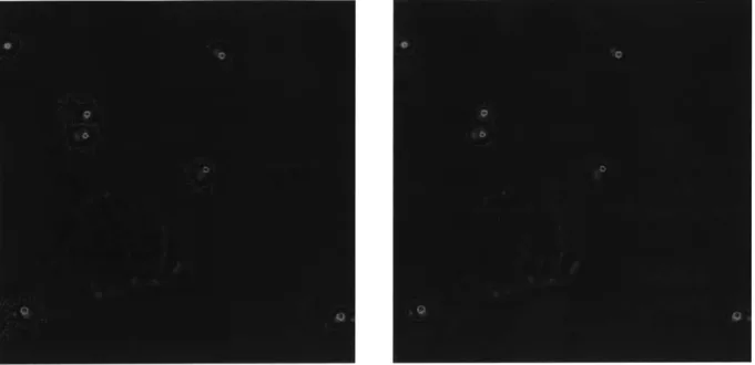
The results of two representative runs of the algorithm on these images are shown in Figure 7. In the runs with bright field images, the noisiness of the original image caused the detected cell borders to also be extremely noisy and jagged, often extending far beyond the actual cell border. The ConA images provided smoother borders for the most part, with some extreme missegmentations, like putting one cell inside another cell. The ConA images

Figure 7: Output of the CellProfiler segmentation algorithm run with the bright field (left) and ConA (right) images as input superimposed on the original bright field image.. Nuclei used as seed regions are outlined in green and detected cell borders are shown in red.

also often had borders which did not align with cell borders, or which extended beyond cell borders.

Results

While this algorithm initially appeared promising, results were not as good as those obtained from thresholding. One possible explanation for the poor quality of cell detection and seg-mentation was the fact that the cells being segmented are yeast cells, while CellProfiler was designed mostly for mammalian cells where most cells are sharing borders with other cells. Yeast cell morphology is significantly different from that of other cells. They are smaller, so small errors in borders affect overall accuracy more, and they are not usually touching on all sides like mammalian cell do, though there are occasional clusters. However, it would be possible in future work with budding yeast cells to adapt this algorithm for their specific cell morphology. It did perform well in determining which objects were actually composed of more than one cell and approximating where the borders might be between them.

4.2.4 Yeast-specific cell detection and segmentation

It is appropriate to look at a cell detection algorithm tailored specifically to yeast cells given the fact that the more general algorithm in the previous section did not perform well due to cell morphology differences. Although there are not many yeast-specific segmentation approaches, one group developed an approach that performed well.

[13]

This approach uses a bright field includes a scheme for cell detection as well as segmentation, both of which rely on the computation of a gradient image. This gradient image helps to eliminate problems of uneven illumination. The segmentation part of the algorithm relies on the detection of candidate cell centers in a cluster of cells and then the use of a polar plot of the cell to find the best cell contours.

This approach shouldn't suffer from the same problems as had been described in subsub-section 4.2.1. It chooses the best cell borders using dynamic programming, which optimizes the choice of a cell border by looking at the whole cell. It avoids the problem of having jagged cell borders by the nature of the dynamic programming approach, and it detects the cells initially by using a method that models noise in the image to eliminate it as a source for errors.

The cell detection process can be outlined as follows:

1. Compute the gradient image from the original bright field image using Prewitt's method.

[7]

2. Find the threshold at which to determine which gradient values are part of the cells and which are noise. This is calculated by fitting the gradient values to a distribution and removing those below a specific value (described in detail below).

4. Perform a morphological opening with a small circular element to remove small struc-tures due to noise.

The output of this algorithm should be a set of cells ready to be segmented. The gradient image is calculated by filtering the image with two masks, one for each direction, to enhance differences in both directions, and then letting the final gradient image be the magnitude of these two filtered images. Then, any pixel with a value above a threshold, which is defined as

#

in the original paper, is assigned to be a part of the foreground.

In order to calculate /, the gradient values below the median are fitted to a Rayleigh distribution function, where there is a parameter o which is varied until the best fit is found. Then,

#

= 7.5o-, which corresponds to designating pixels with gradient values more than 6 standard deviations larger than the mean of the estimated distribution of background pixels as a part of the foreground. This scheme relies on the assumption that the distribution of noise in the background regions of the image are approximately normally distributed.

Once the cells have been detected from their backgrounds, the cells must then be seg-mented. The segmentation algorithm is outlined below:

1. Find candidate cell centers from the segmented image.

2. Create a polar plot of the cell from each candidate cell center.

3. Use dynamic programming with global constraints to choose an an optimal path from left to right on the polar plot. The original plot is repeated three times and the final chosen path is taken from the center repetition of the plot to ensure that the chosen path is closed.

There are multiple ways to choose candidate cell centers depending on how clustered the cells are. If the clusters are no larger than 3 or 4 cells in each cluster, then a simple distance

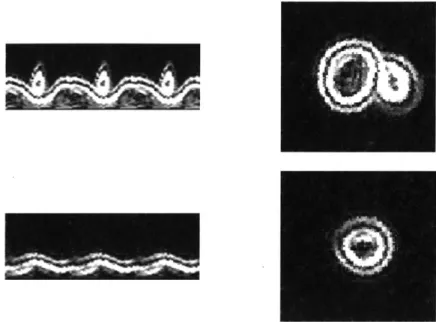
a

Figure 8: An example polar plot of two yeast cells calculated from the gradient image. This would have the dynamic programming algorithm run on it to find an optimal path

transform on the cell mask can be used, and the local maxima are considered to be candidate cell centers, which is a good choice for this dataset.

The polar plot from the candidate cell centers is then created by sampling rays outward at 30 equally spaced radial points. Then using this plot a cell contour can be extracted. The dynamic programming scheme uses constraints to ensure convexity for the majority of the cell, so it penalizes transitions in the polar plot which correspond to right turns. It does ensure that the extracted contour is closed by going around the cell three times. This algorithm should perform well even when the calculated candidate cell center is quite off-center.

Results

This approach relied on the ability to segment the cells by calculating the gradient image and then choosing a cutoff value from this image to determine which parts of the image were edges. However, it did not detect cell edges such that the cells could be filled in in the way that the algorithm describes. The cells were not even close to having closed outlines. To test if it was simply a problem of fitting the data correctly, the best value for

#

was chosen

manually for several images. However, the output was still not ideal. There was still the problem of the two detected edges for each cell wall as was discussed in earlier approaches to cell detection. It is difficult to know which cell edge to choose. Then, with the choice of

#,

it is not possible to guarantee that only one set of edges is included in the thresholded images, or that both sets of edges are included. Some partial edges are included, and in some cases, an entire outer edge is thresholded out. Finally, any partial outer edges which were detected are then removed with the morphological opening. This leads to a great deal of inconsistency in the final detected cells: some include the outer edges, and some don't. In cells with small buds, the buds are often lost as can be seen in the figure.

Figure 9: Yeast-specific cell detection algorithm to detect cells. A threshold value # was chosen manually for this set of images

This poor performance is most likely related to some of the assumptions made in the original paper about the distribution of noise in the image, and how it can be fit to a distribution. Though it claims that these assumptions are "crude", it says that they still allow the algorithm to perform well. This was not able to be reproduced, perhaps even due to some difference in the distribution of pixel values in the original data.

Then, the second part of the scheme to segment cells was not implemented as a result of the failure of the first part. Though it could have been attempted using cells detected using other methods, it wasn't a worthwhile endeavor given the fact that the first part completely failed. The paper did admit that the only incorrectly detected cell contours were buds, which are important in this case. Though there was a proposed solution to this problem, it was

not tested.

4.3

Nucleus detection and segmentation

The nuclei of the cells must also be detected and segmented in addition to the cells them-selves. The cells, which were stained with ConA, were also stained with DAPI, a fluorescent stain which binds to A-T rich regions of DNA. This problem is relatively straightforward in comparison to that of segmenting cells, since the nuclei are never touching each other and clustered.

The algorithm to detect nuclei is outlined below, and the code can be found in appendix 7.C

1. Use morphological opening to calculate the background of the image 2. Subtract this calculated background from the original image

3. Threshold out the nuclei to get a nuclear mask 4. Remove any objects which are too big to be nuclei

5. Dilate the nuclear mask since this thresholding tends to underestimate nuclear bound-aries

First the background of the image is calculated using morphological opening with a disk of radius 6. This removes any objects in the image which are smaller or thinner than the disk, which effectively removes all of the nuclei in the image. This then leaves only the background noise of the image, and any uneven illumination. This background calculation is important because in examining the nuclei, the intensity of the stain is important and can indicate the amount of DNA in the nucleus. Removal of the background ensures consistent intensity calculations. This step also helps to deal with one of the problems that can arise

with the DAPI staining: occasionally the entire cell will get stained with DAPI and the entire cell will fluoresce, or a much larger part of the cell will get stained with DAPI. These regions, which are larger than nuclei will, for the most part, be included in the background. Then, they will be removed in the next step when the background is subtracted from the original image.

Once the background has been removed, the nuclei are thresholded out to create a nuclear mask. Then, any objects which are larger than 100 pixels are removed from the mask. This represents a nucleus with a radius of 6 pixels, which is the same as the disk size that was used for the morphological opening. Any nucleus should be much smaller than this. This step ensures that any nuclei which had problems with the DAPI staining are not included in the mask.

In this nuclear detection code the DAPI channel is modified to remove any objects which are not nuclei, and to remove any background noise. In the last step, the nuclear mask is then dilated to make sure that the entire nucleus is included in the final modified image. It is not as important to get the nuclear outline perfect as it is to ensure that the entire nucleus is included in the mask, since the overall intensity of the nucleus is important, so the image is dilated several times with a disk of radius 1.

In later steps in the workflow, the DAPI images will be combined with the segmented cells, and any nuclei which are not contained within cells will not be included in calculations. While it would be possible to start with a cell mask and then to look for a nucleus within the mask by performing operations locally, it is more simple and quite effective to do the operation for the entire image and apply the mask later. This order of operations also allows for the background intensity correction to occur for the entire image.

4.4

Discussion

An ideal cell detection and segmentation algorithm would be able to identify only the parts of an image which are cells using smooth contours, and then correctly segment them. It would not leave out the contours of any buds, since those are necessary for cell cycle stage classification. It would also be precise in the detection of cell outlines, since this is necessary for calculating GFP intensity in the investigation into the response to DNA damage. An ideal algorithm would be able to segment even large clusters of cells so that any type of data could be used, with either dense cells or with sparse cells. Most importantly, the algorithm would be consistent in the way it detects and segments cells.

The only approach that satisfied the majority of these requirements was that of using the ConA images with thresholding. This approach was selected because of its consistency and simplicity. The use of the ConA images completely eliminates the problem of cell wall thickness creating multiple edges, and thresholding is a reliable method of detection. Its drawback is that the images of cells must not contain large clusters, since these cannot be handled and will be ignored. This means that sparse images with dilute cells must be used.

It might be possible to combine the ConA thresholding approach with one of those which performs segmentation by modifying both. However, it is possible that more complicated approaches such as that from subsubsection 4.2.4 might not perform better in this context given the emphasis placed on bud detection. Once the rest of the methods are completely developed and tested, it will be possible to work on the cell detection and segmentation part of the workflow further to allow a wider variety of data to be able to be used as input.

5

Cell Cycle Stage Classification

It can be seen from the paper by Jelinsky, et al. that the budding yeast cellular response to DNA damaging agents is dramatically affected by the cell's position in the cell cycle at the time of exposure. [10] Therefore it is important that the cell cycle stage of individual cells can be determined from the images of cells.

In their approach, populations of cells were arrested in various cell cycle stages and then analyzed using oligonucleotide probes. With images of the cell in this work flow, more data can be obtained than simply amount of expression of a gene, since the images can be analyzed and amount and localization of protein using the GFP tagged proteins can be determined. However, in order to combine this information with that about cell cycle stage, the cell must be classified. While it is possible to arrest cells in various stages of the cell cycle, this process can affect cell morphology and state, compromising the detection and classification approach. (see subsubsection 5.4.2) Rather than taking this approach, supervised learning and classification of cells from a wild-type, unsynchronized population is more appropriate.

First, a descriptive set of cell features must be created which will allow the cells to be classified. The cells should be able to be classified as being in one of three stages of the cell cycle: G1, S, or G2/M. Then a manually-curated training set of cells must be created for

training as well as for validation steps. Finally, the remaining cells can be classified.

G1

S G2/M

anaphase telophase

5.1

Creation of a training set

A training set of data must be created in order to train neural nets. It is also useful to have a set of labelled cells to validate the features and to make sure that the calculated values are consistent with what would be expected for cells in the different stages of the cell cycle. In order to do this, a MATLAB interface was created which allows a user to manually label cells. To ensure that a representative set of cells were included in the training set, the input to this interface is a directory of images of yeast cells and cell masks generated from the program described in subsubsection 4.2.2. The user can then choose the number of cells from each image to label. Then the user is presented with that number of randomly selected cells from each image. The code displays a superposition of the original ConA image of the cell and the DAPI image of the DNA in the cell. In general, a combination of bud size and nuclear size, position, and intensity is enough for a human to accurately and easily label a cell. Cells which had just undergone G2/M and were then in G1 but still connected and not segmented were classified as a single cell in G1, since they are known to be in the same stage

of the cell cycle and have just finished dividing. If the image with which the user is presented contains more than one cell, the user can designate it as an invalid cell segmentation. This will allow later identification of clusters of cells which were incorrectly segmented and make sure that they are not included in data about single cells.

In the images, there are generally more cells in the G1 and S stages than there are in the

G2/M phase, since the cell spends such a small amount of time in G2/M before it becomes a

mother and daughter cell in G1 again. This led to an unequal number of cells in the different stages of the cell cycle. Generating enough labels for cells creates a large enough data set that the small percentage of G2/M cells still has enough data points for the training of a neural net.

these, 62% were G1, 28% were S,6% were G2/M, and 4% were classified as invalid cells.

5.2

Feature selection

In order to classify cells automatically, a set of features must be chosen and calculated. 14 features were chosen to give the information necessary. These include features that describe the size and geometry of the cells. In order to make sure that the features that were chosen do, in fact, give useful information about the cells, other cell classification schemes were investigated and their feature lists examined.

[1]

Source Image(s) Feature Name Feature Definition

Area Cellular area

Convex Area Area contained in the convex hull of the cell Solidity/Convexity coArea _ConvexArea-- 1 for a convex cell

Perimeter Cellular perimeter

ConA Form Factor 47rfre = 1 for a perfectly circular cell

Major Axis Length Major axis length of the ellipse that is the best fit to the cell

Minor Axis Length Minor axis of the best fit ellipse

Eccentricity Ratio of the distance between the foci of the best fit ellipse and its major axis length

Bud size Size of the bud (see 5.3.2)

Ellipticity Residual of the best-fit ellipse divided by the number of pixels in the cell boundary that was fit

Nuclear Area Area of the detected nucleus

Number of nuclei Number of nuclei in the given cell mask

DNA Average Intensity _{Intensity of the detected DNA averaged over}

all pixels in the nucleus

Overall Intensity Sum of the intensity values at each pixel in (Amount of DNA) the nucleus

Table 1: List of features calculated for each cell for classification and which images they are derived from

These features lists gave a good baseline for the maximum number of features a classifi-cation process might want to use. These were then pared down to features which included information about cell morphology - information about cell texture or protein intensity is not related to the problem of cell cycle stage classification and therefore unnecessary.

Once these generalized feature lists had been consulted and modified, some budding yeast-specific features were added. The main such feature was bud size, which is one feature that is key to determining cell-cycle stage, since when a cell is in G1, it has no bud, while

in S, it has a bud of increasing size, and in G₂/M, the bud is nearly the same size as the original mother cell. Another yeast-specific feature which was added was the number of nuclei in the cell. This was added because, as was indicated in the previous section, sometimes the detected cells are actually doublets which have just finished G2/M and have not fully separated. This feature was included to help identify these cells. In Table 2 and Table 3 a probable scheme for differentiating between the cell cycle stages is shown using the chosen features.

The final feature list can be seen in Table 1. This shows the images which are used to generate those particular features as well as the exact description of the features.

Table 2:

Feature G1 G2

DNA Intensity n 2n

Nuclear position Centered Towards bud

Cell Area n > 1.3n

Bud Size < 70% mother cell size > 70% mother cell size

Differentiation between G1 and G2 using a subset of the selected features

5.3

Feature calculation

The output of the cell and nuclear detection programs described in section 4 was used to calculate the selected cell features in MATLAB. These were then saved in csv files to be

Feature G1 S G2

DNA Intensity n n - 2n 2n

Nuclear position Centered Towards bud Towards bud or split between 2 cells

Cell Area n 1.3n > 1.5

Bud Size < 10% mother cell size < 70% mother cell size > 70% mother cell size Table 3: Differentiation between G1, S and G2/M using a subset of the selected features

used for later data analysis as well as for input for classification.

5.3.1 Basic cell features

The basic cell features were calculated using MATLAB's regionprops function. This function takes in a black and white image mask and an image of values for each pixel as well. Each cell in the black and white image is considered to be a connected component, for which MATLAB calculates its own sets of values. Specifically, the values for cell area, convex area, perimeter, major axis length, minor axis length, and cell eccentricity are all calculated directly from this function. Then the features solidity and form factor are be calculated directly from these values.

Once the basic cell features have been calculated for a particular cell, that cell's mask is applied to the mask of cell nuclei to obtain an image with only the nuclei of the current cell. Then, the function regionprops is used once again on this image along with the DAPI image to calculate nuclear intensity, average nuclear intensity, number of nuclei, and nuclear intensity.

5.3.2 Bud detection

Along with DNA intensity, bud size is the most descriptive feature about a budding cell when determining cell cycle stage. This makes it one of the most important features to calculate

as input for classification.

Bud detection is challenging in that budding yeast cells have irregular shapes. They are not perfect circles nor are they perfect ellipses, and occasionally the cell segmentation might introduce some errors which add to the irregularity. The detection algorithm must be able to determine whether or not a cell has a bud, or whether any irregularities in the cell contours are simply a part of the cell's shape. Then, if a cell does, in fact have a bud, it must be able to determine which of these irregularities is actually a part of a bud. Finally, it must be able to measure the size of the bud. A number of approaches to bud detection were tested, and the best and most accurate selected.

Bud detection using polar plots

If a yeast cell with no bud is viewed as an ellipse, then the bud of a yeast cell would simply be an irregularity in this ellipse. If the approximate center of the cell is found, then a polar radial plot of the cell can be created by sampling the radius at equally spaced points around the cell. While this plot of a cell should have few irregularities, the plot of a budded cell will have a clear point at which there is a bud.

This bud detection algorithm calculates this radial plot and finds the largest peak, which should be the bud. Then, it finds the two local minima nearby, which should be the beginning and end of the bud. It then uses these values to segment the bud from the mother cell. While this method performs reasonably well, it can discount buds which are small on cells which are very elliptical. In these cells, a point along the major axis is the maximum point in the radial plot and is chosen as the bud, while the bud remains ignored because it is a smaller local maximum.

Bud detection using polar plots - fitting to an ellipse

If instead of simply creating a plot of the cell's radii out from the cell center and looking for the maximum radius, the cell is fitted to an ellipse, then the accuracy of bud detection

can be increased significantly. In order to locate the bud, the data for an ellipse equivalent to the cell with no bud can be generated and compared to the actual cell data. Using this comparison, the angular location of the bud can be found.

fitted ellipse

radii differences

Figure 11: Cell undergoing bud detection. The candidate cell center is marked in the top left image. The bottom left image shows the calculated radii out from the cell center, with the top right showing the ellipse that was fitted to the cell, and the bottom right showing the difference between the calculated radii and the fitted ellipse. This clearly shows a bud at the correct position.

The bud detection algorithm is outlined here, and the code can be found in subsection 7.E

1. Compute the distance transform on the cell and then find the maximum value to find the candidate cell center.

2. From this cell center, find the radius of the cell at 5 degree increments around the entire cell in order to create a polar plot of angle vs. radius.

3. Smooth this radius plot to remove small irregularities in the cell as well as small discontinuities due to the fact that the radius is only sampled every 5 degrees.

4. Find the local minima in this radial plot. These should be the minor axes of the ellipse. Designate their mean to be the minor axis length, b.