EvoEvo Deliverable 2.5 : Specifications of the realistic network model

HAL Id: hal-01577142

https://hal.archives-ouvertes.fr/hal-01577142

Submitted on 24 Aug 2017

HAL is a multi-disciplinary open access archive for the deposit and dissemination of sci-entific research documents, whether they are pub-lished or not. The documents may come from teaching and research institutions in France or abroad, or from public or private research centers.

L’archive ouverte pluridisciplinaire HAL, est destinée au dépôt et à la diffusion de documents scientifiques de niveau recherche, publiés ou non, émanant des établissements d’enseignement et de recherche français ou étrangers, des laboratoires publics ou privés.

To cite this version:

Guillaume Beslon, Carole Knibbe, Charles Rocabert. EvoEvo Deliverable 2.5 : Specifications of the realistic network model. [Research Report] INRIA Grenoble - Rhône-Alpes. 2014. �hal-01577142�

Page 1 of 14

EvoEvo Deliverable 2.5

Specifications of the realistic network model

Due date: M6 (June 2014)

Person in charge: Guillaume Beslon

Partner in charge: INRIA

Workpackage: WP2 (Development of an integrated modelling platform)

Deliverable description: Specifications of the realistic network model: Description of the modeling choices for the realistic genetic/metabolic network model. This model should include a realistic cellular network model suitable for the study of network variability, robustness and evolvability.

Revisions:

Revision no. Revision description Date Person in charge

1.0 First version of the realistic network model 03/09/14 C. Rocabert (INRIA)

1.1 Corrections by G. Beslon and C.Rocabert 09/10/14 C. Rocabert (INRIA)

Page 2 of 14

Table of Contents

1.

2.

2.1.

2.2.

3.

3.2.

4.

6.

Page 3 of 14

1. Introduction

The objective of WP2 is to produce an integrated model able to decipher the contribution of the different levels of organization that interact to produce a microorganism. To do so, WP2 is organized in four parallel tasks.

Deliverables 2.1 and 2.3 focused on the genome, the metabolic network and the population levels (thoses documents are available on www.evoevo.eu). Deliverable 2.5 offers to focus on a more realistic representation of the biochemistry, based on the artificial chemistry (Achem) developed in previous models, in order to produce a realistic genetic regulation network. Indeed, complex situations, such as cooperative/competitive binding of transcription factors, stochastic effects due to small enzyme or transcription factor concentrations, or competitive effects between different binding sites, have been shown to interact with the evolutionary process.

The main difficulty here is to propose a realistic enough modeling scheme and simultaneously to keep the computational complexity low enough for the model to be computable in a reasonable time.

On the basis of formalisms used in deliverables 2.1 and 2.3 (mainly the Pearls-on-a-String formalism), this model must contain at least:

• A realistic genetic regulation network (GRN), • A model of stochasticity of gene expression (SGE),

• A coupling between the genetic network and the metabolic network to allow sensing. This deliverable is built in three parts. The first part reminds the knowhow of Inria and University of Utrecht (UU) with regard to GRN models. In the second part, the new GRN formalism is detailed. In a third part, models of transcription noise and genetic-metabolic networks coupling are introduced.

2. Background

The GRN model presented here is strongly rooted in the knowhow of Inria and UU. Models developed by each partner are presented above.

2.1. Overview of the Pearls-on-a-String model

In the GRN model developed by UU (see Crombach & Hogeweg, 2008, for a complete description of it), the network of each individual consists of genes with interactions among them. A gene has a state of expression 𝑠 (on = 1, off = 0), a threshold 𝜃   ∈ −2, 1, 0, 1, 2 and an identification tag 𝑡 ∈ 0, 1, 2, … , 𝑛 . A gene may be regulated by binding sites located directly upstream from the gene. Binding sites specify which transcription factor may bind to them via their own identification tag (i.e. if tags are equal), which is called the binding preference. They also determine the type of interaction 𝑤: activation (𝑤   =  1) or inhibition (𝑤   =   −1). If there are multiple copies of a binding site present in the upstream region of a gene, there will be parallel edges in the resulting network. Symmetrically, if there are multiple copies of a gene, they all bind to a binding site (see figure 1).

Page 4 of 14

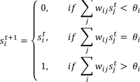
On this network the gene expression dynamics are defined. Like in classical boolean networks, the genes in the network are updated in parallel. However, as it is a threshold network, the activity of the gene 𝑖 depends on its threshold 𝜃_!. Then, its state of expression 𝑠_! at time 𝑡 + 1 is defined as:

𝑠_!!!! = 0, 𝑖𝑓   𝑤!"𝑠!! <   𝜃! ! 𝑠_!!, 𝑖𝑓   𝑤!"𝑠!! =   𝜃! ! 1, 𝑖𝑓   𝑤_!"𝑠_!! _{>   𝜃} ! !

The fitness of each individual is then computed depending on which genes are on or off.

Figure 1 - Overview of Pearls-on-a-String model (from Crombach & Hogeweg, 2008). (A) Simulations are run on a 150x50 lattice for 6.105 time steps. The lattice harbors a population of genomes, where a genome is a linear chromosome of genes with binding sites. A Boolean threshold network is built from each genome. During each time step the network may update the expression level of the genes for 11 propagation steps. (B) The impact of several gene and binding site mutations is shown. The change in the genome and network topology is signaled by a red star. In a typical simulation the parameters are (per gene, binding site): gene duplication (dup) 2.10-4, deletion 3.10-4, threshold 5.10-6, binding site (bsite) duplication 2.10-5, innovation 1.10-5, deletion (del) 3.10-5, preference (pref) 2.10-5 and weight 2.10-5. (C) Typically the environment changes over time with a probability of λ = 3.10-4. The two evolutionary targets A and B determine which genes should be expressed (on) or inhibited (off). The result is four categories of genes; some should be always on, some should toggle their expression state and some should never be expressed. In a typical simulation, the target expression states are, from gene 0 to 19, A: 00011 11000 00000 11111 and B: 11010 01001 01100 01011.

2.2. Overview of the R-Aevol model

R-Aevol (Regulation-Artificial evolution, Beslon et al., 2010b) is an extension of Aevol platform (see Knibbe et al., 2007 for a description of Aevol) that includes a model of prokaryotic regulation in the artificial chemistry. To model the interactions between transcription factors and promoters, two binding sites are defined for each promoter: Preceding the promoter, the enhancer site will allow TFs that bind to it to increase the transcriptional activity. The operator site, directly following the promoter, will on the contrary produce a down-regulation of the promoter’s activity whenever a TF binds to it.

Page 5 of 14

A promoter owns a basal expression level 𝛽!, which depends on how close its sequence is to a

consensus sequence. The transcriptional activity of a promoter depends on the combined activity of the transcription factors that activate it, following:

𝐴! 𝑡 =   𝑐! 𝑡 𝐴!" !

and of those that inhibit it, following:

𝐼! 𝑡 =   𝑐! 𝑡 𝐼!" !

𝐴!" (resp. 𝐼!") being the affinity of protein 𝑗 with the enhancer site of the promoter 𝑖 (resp. on its

operator) and 𝑐_!(𝑡), the concentration of protein 𝑗 at time 𝑡.

The transcription rate 𝑒_! over time of an RNA is then given by the Hill-like function:

𝑒! 𝑡 =   𝛽!  . 𝜃! 𝐼! 𝑡 !+ 𝜃!  . 1 +   1 𝛽!− 1 𝐴_! 𝑡 ! 𝐴! 𝑡 !+ 𝜃!

where n and 𝜃 are constant coefficients that determine the shape of the Hill-function. Finally, given the transcription rate, one can compute the protein concentration (for simplicity, it is assumed that the protein concentration is linearly proportional to the RNA concentration) through a synthesis-degradation rule:

𝑐! 0 =   𝛽!      

𝜕𝑐_!

𝜕𝑡 = 𝑒! 𝑡 − 𝜙𝑐!(𝑡)

where 𝜙 is a temporal scaling constant representing the protein degradation rate.

Thus, when a gene is regulated, the concentration of its product is scaled up or down depending on its transcription rate.

3. Presentation of the realistic network model

In deliverables 2.1 and 2.3, individuals own genomes made of two types of pearls:

• pearls being functional genes, and coding for enzymatic reactions in the metabolic network,

• pearls being pseudogenes (non coding part of the genome).

The Pearls-on-a-String model described above is an obvious basis to develop a GRN, as exemplified in Crombach & Hogeweg (2008). Yet, the boolean network formalism lacks precision, since protein concentrations cannot vary continuously. Moreover, the regulation activity is encoded in the binding sites, independently of their position relatively to the promoter. In this sense, R-Aevol model should help us to develop a more realistic approach. Merging both formalisms allows us to

Page 6 of 14

exploit the regulation scheme developed in R-Aevol, keeping the model simple enough by transposing it in the Pearls-on-a-String scheme.

3.1. Description of the genome structure

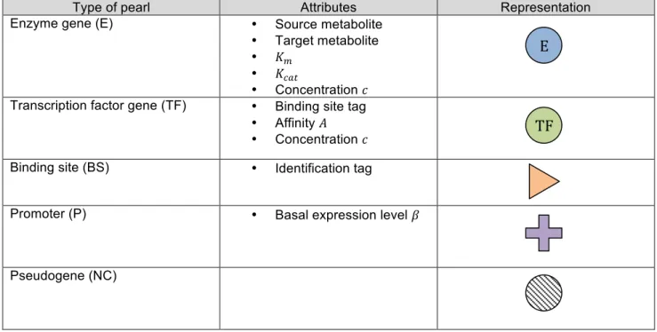
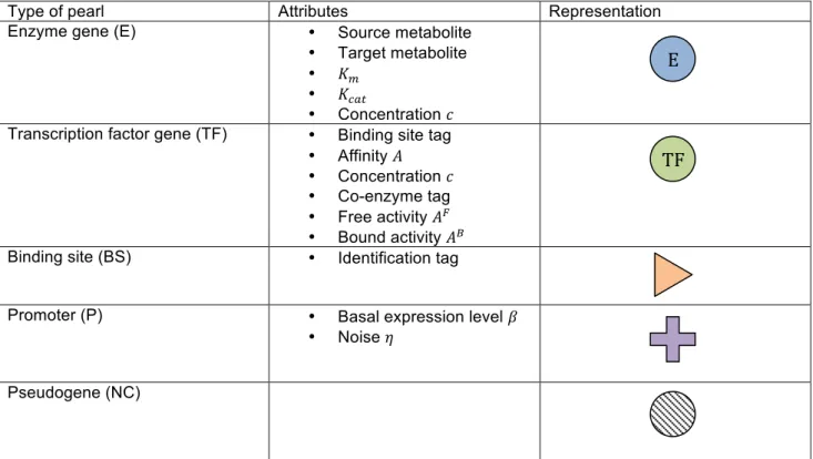
Compared to previous deliverables, the genome structure is enriched by three new types of pearl (table 1).

There are now five types of pearls:

(1) Genes coding for enzymes in the metabolic network (type E). Those genes code for enzymatic reactions, described by the following Michaelis-Menten equation:

𝑑[𝑝] 𝑑𝑡 =

𝑘_!"#  . [𝐸]  . [𝑠]

𝑘!+ [𝑠]

where 𝑠, 𝑝, 𝑘!"# and 𝑘! are attributes of the gene, [𝑠] and [𝑝] are the concentrations of the

metabolites (see deliverable 2.1 for details on the metabolic network model), and [𝐸] is the enzymatic concentration (here, we assume that the concentration of free enzymes [𝐸] is always equal to the total concentration [𝐸!], i.e. the concentration of combined enzymes [𝐸𝑆] is always

close enough to zero. In this case, Michaelis-Menten dynamics are slightly biased, but it strongly reduces the number of equations to solve).

(2) Genes coding for transcription factors (type TF). Each transcription factor 𝑖 owns an identification tag which designates a binding site 𝑗, and an affinity 𝐴_!" for this binding site.

(3) Binding sites (type BS) specify which transcription factor may bind to them via their own identification tag.

(4) Promoters (type P) determine where the transcription should start. Each promoter 𝑖 owns a basal expression level 𝛽_!.

(5) Pseudogenes (type NC) constitute the non coding part of the genome and drift in the attributes space. A pseudogene can be restored with some probability into one of the four active pearls.

Page 7 of 14

Type of pearl Attributes Representation

Enzyme gene (E) _• Source metabolite

• Target metabolite • 𝐾!  

• 𝐾!"#  

• Concentration 𝑐   Transcription factor gene (TF) _• Binding site tag

• Affinity 𝐴 • Concentration 𝑐

Binding site (BS) _• Identification tag

Promoter (P) _• Basal expression level 𝛽

Pseudogene (NC)

Table 1 - Types of pearl in the basic network model

Binding sites directly flanking a promoter regulate its transcriptional activity. The enhancer site directly precedes the promoter and is made of one or more contiguous binding sites. The operator site directly follows the promoter and is also made of one or more contiguous binding sites. TFs that bind to a binding site in the enhancer site will increase the transcriptional activity. On the opposite, TFs that bind to a binding site in the operator site down-regulate the promoter activity (see figure 2). As in R-Aevol, a promoter has a basal level activity 𝛽 and regulation sites are not mandatory, or can be present separately.

Figure 2 – Typical structure of a functional region in the genome. It starts with a promoter, possibly flanked by an enhancer site and/or an operator site (e.g. here, the enhancer site is made of one binding site, and the operator site is made of two binding sites). All contiguous functional genes following the operator site are transcribed. The first pearl of another type interrupts the transcription (here a piece of non coding DNA). In this case, the functional region is an operon, because several genes are controlled by one unit of regulation.

TF" E" Enhancer"site,"made" of"one"binding"site" Promoter" Operator"site," made"of"two" binding"sites" Two"genes"(one" coding"for"a" transcription"factor" and"one"for"an" enzyme)"constitute" an"operon" Circular"single" strand"genome"

E

TF

Page 8 of 14

All functional genes following the operator site are transcribed, thereby allowing for operons. Downstream of the operator site, any pearl other than TF or E makes the transcription stop (figure 2). To be functional (figure 3), the promoter can be flanked by binding sites or not, but functional genes must immediately follow the regulation unit (enhancer site + promoter + operator site).

Figure 3 – (A) Some examples of pearl’s combinations giving a functional region. The promoter can be flanked by binding sites or not, but functional genes must immediately follow the regulation unit (enhancer + promoter + operator). (B) Some examples of wrong pearl’s combinations. On left, a non coding pearl interrupts the transcription before the functional gene. On right, the promoter is missing.

The genome undergoes mutations during replication. Point mutations affect the attributes of each pearl with a probability per pearl defined at the beginning of the simulation. Every attributes of every type of pearl can mutate, even for the pseudogenes, giving some interesting evolvability properties (since pseudogenes attributes can travel in the neutral landscape). A point mutation can transform an active type into a pseudogene (active types are TF, E, BS and P). Pseudogenes can be restored into one or another active type with some probabilities, however it is impossible to mutate directly from an active type to another (see figure 4).

The genome also undergoes chromosomal rearrangements (duplications, deletions, translocations, inversions), that can affect the structure of functional regions and the proportion of non coding DNA (see deliverable 2.1 for details).

E" E" TF" E" E" Some%func*onal%combina*ons%of%pearls% func*onal%region%

(A)%

(B)%

Page 9 of 14 Figure 4 – Different mutation rates define the probability to switch from one pearl’s type to another. Active types – binding sites (BS), transcription factors (TF), enzymes (E) and promoters (P) – can only become pseudogenes (with probability

ppseudo). Sometimes, a pseudogene can be restored to one type or another depending on four mutations rates: pBS is the

probability to become a binding site (resp. for pPROM, pE and pTF). In summary, 5 mutation rates define transitions

between pearl’s types.

3.2. Description of the genetic regulation network

In the previous chapter, we merged the boolean GRN formalism used in the Pearls-on-a-String model with the R-Aevol formalism. From the genetic structure described above, one can deduce the regulatory network as following:

(1) The activity 𝐴!(𝑡) of each binding site 𝑠 is:

𝐴_!(𝑡) =   𝑐_! 𝑡 𝐴_!"

!

with 𝑐!(𝑡) the concentration of the transcription factor 𝑗 at time 𝑡 and 𝐴!" the affinity of this

transcription factor for the binding site 𝑠.

(2) From (1), we deduce the activity of the enhancer site 𝐸!(𝑡) and of the operator site 𝑂!(𝑡)

flanking the promoter 𝑖:

𝐸_! 𝑡 = 𝐴_!(𝑡)

!  ∈  !"!!"#$%!

𝑂! 𝑡 = 𝐴!(𝑡)

!  ∈  !"#$%&!$!

(3) Then, the transcription rate 𝑒_! over time of the promoter 𝑖 is given by the Hill-like function:

𝑒! 𝑡 =   𝛽!  . 𝜃! 𝑂! 𝑡 !+ 𝜃!  . 1 +   1 𝛽!− 1 𝐸_! 𝑡 ! 𝐸! 𝑡 !+ 𝜃!

E"

TF"

Page 10 of 14

with 𝛽! the basal expression level of the promoter 𝑖, 𝑛 and 𝜃 being constant coefficients that

determine the shape of the Hill function.

The transcription rate 𝑒! is applied to each functional gene being controlled by the promoter 𝑖, such

that each protein product (enzyme or transcription factor) has its own concentration regulated through a synthesis-degradation rule, depending on 𝑒!:

𝑐! 0 =   𝛽!      

𝜕𝑐_!

𝜕𝑡 = 𝑒! 𝑡 − 𝜙𝑐!(𝑡)

where 𝜙 is a temporal scaling constant representing the protein degradation rate.

4. Adding transcriptional noise in the genetic regulation network

In the cellular environment, some reactant numbers, like enzymes or transcription factors, tend to be of low order (10-100). In this case, the stochastic effects due to reactant population size become predominant, as it is specially the case during gene expression (Elowitz et al. 2002). Thus, the analysis of genetic regulation networks is complicated by fluctuations associated with discrete reaction events in small-number reactant pools. Even if deterministic models are often sufficient to describe those processes, in many examples, they fail to capture essential features of the underlying stochastic system (see Kaern et al., 2005, for a review).

Several mathematical models deal with the fundamental stochastic nature of biochemical reactions, from discrete and stochastic models (SSA, Tau-leaping, CME) to continuous and stochastic ones (mainly the Chemical Langevin equation, CLE), see Gillespie et al. (2013) for a review. Unfortunately, even if discrete models are more realistic, they are computationaly very costly and cannot be used in the case of an integrated model of evolution. We opted here for a continuous and stochastic model, by using stochastic differential equations (SDE). In this case, the assumption is made that the deterministic equations can be meaningfully separated from the stochastic fluctuations. The method consists in adding a random white noise term 𝜉(𝑡) to the deterministic equations describing protein concentrations seen above (Scott, 2006). Many experimental studies agree with the fact that stochasticity in gene expression (SGE) mainly comes from stochasticity during transcription (Newman et al. 2006). Moreover, the structure of the promoter plays a major role in the noise strengh (e.g. depending on the presence of a TATA box in eukaryotes). In prokaryotes, it is also recognized that promoters play a central role, and that their noise strengh is somehow encoded in their structure and sequence (e.g. in Roberts et al., 2011). Let’s consider that the transcriptional noise is genetically encoded in the promoter. In the Pearls-on-a-String formalism, this comes down to adding a noise attribute 𝜂 to the promoter type. 𝜂 mutates as all others attributes of the pearl, allowing for evolution of the SGE. Then the evolution of the transcription rate 𝑒! in time of each promoter 𝑖 becomes:

𝑒! 𝑡 =   𝛽!  . 𝜃! 𝑂! 𝑡 !+ 𝜃!  . 1 +   1 𝛽!− 1 𝐸_! 𝑡 ! 𝐸! 𝑡 !+ 𝜃! + 𝜉!(𝑡)

Page 11 of 14

Since stochasticity is inevitable (the cell cannot escape the physical and chemical laws), a minimal noise 𝜂_! exists such that 𝜂_! ≥ 𝜂_!.

5. Coupling the genetic and metabolic networks

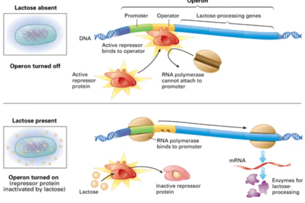
Bacteria are able to sense their environment by detecting the presence of a particular molecule or signal, and to give an appropriate answer by updating their genes expression profile. A famous example of this behaviour is the lactose operon, described for the first time by François Jacob, Jacques Monod and André Lwoff.

The lactose operon is made of three genes (lacZ, lacY and lacA), that are controlled by one promoter flanked by an operator. An other gene, lacI, codes for a transcription factor which inhibates the operon by binding on the operator. LacI is a constituent gene, meaning that it is always expressed, but its affinity for the operator is modified in presence of lactose. Then, in absence of lactose, lacI is active and down-regulates lactose operon expression by binding on the operon. If lactose is present, it represses lacI activity (by binding on it). In this case, lactose operon is expressed and the cell is able to metabolize lactose (see figure 5).

Figure 5 – (From http://apps.cmsfq.edu.ec/biologyexploringlife/) The lactose operon is inactive in the absence of lactose (top) because a repressor blocks attachment of RNA polymerase to the promoter. With lactose present (bottom), the repressor is inactivated, and transcription of lactose-processing genes proceeds.

More generally, co-enzymes can repress or activate transcription factors activity (they are repressors or activators). This very important biological feature is introduced in the realistic network model by adding three attributes to the transcription factor type (TF):

Page 12 of 14

• A co-enzyme identification tag (in the metabolic space [1, +∞[), • A free activity (𝑡𝑟𝑢𝑒 or 𝑓𝑎𝑙𝑠𝑒),

• A bound activity (𝑡𝑟𝑢𝑒 or 𝑓𝑎𝑙𝑠𝑒).

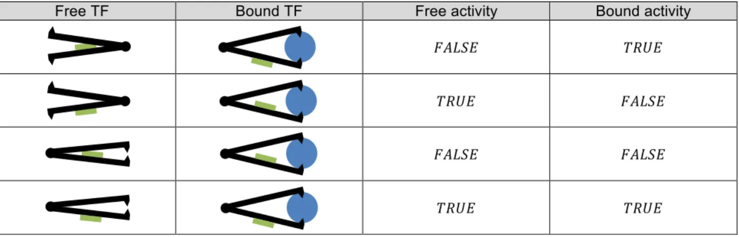
A metabolite 𝑚   ∈ [1, +∞[  can bind to the TF as a co-enzyme, and be a repressor or an activator. The combination of the free activity and the bound activity gives rise to four type of behaviours, as described in table 2. A TF can be viewed as a protein which can have two conformations: one when the TF is free, and another when a co-enzyme bind to it. This behaviour is represented in table 2 by drawing a TF as a structure with two arms linked by a pivotal point. The active site of the TF is located on one arm, and its exposure depends on the equilibrium state (or conformation) of the structure. Two configurations exist: one when the TF is free, another when a co-enzyme bind to the TF thanks to anchoring points located at the end of the arms.

(1) If the TF has no free activity, and has a bound activity, the co-enzyme acts as an activator, (2) If the TF has free activity, and has no bound activity, the co-enzyme acts as a repressor,

(3) If the TF has no free activity neither bound activity, the co-enzyme has no effect. The TF is never active.

(4) Finally, if the TF has free activity and bound activity, the TF is always active, whenever a co-enzyme bind to it or not.

Free TF Bound TF Free activity Bound activity

𝐹𝐴𝐿𝑆𝐸 𝑇𝑅𝑈𝐸

𝑇𝑅𝑈𝐸 𝐹𝐴𝐿𝑆𝐸

𝐹𝐴𝐿𝑆𝐸 𝐹𝐴𝐿𝑆𝐸

𝑇𝑅𝑈𝐸 𝑇𝑅𝑈𝐸

Table 2 – The TF is represented in black, its active site (the part which allow the TF to bind on the binding site) being represented in green. Depending on free and bound activities, the co-enzyme (in blue) acts as an activator or a

repressor, and the active site is free to bind to the binding site or not.

Let’s 𝑐!(𝑡) be the concentration of the TF 𝑖 at time 𝑡 and 𝑐𝑜𝐸!(𝑡) the concentration of its co-enzyme.

Depending on the state of the free activity 𝐴_!! and the bound activity 𝐴_!!, the concentration of the TF 𝑖 that is active  𝑎!(𝑡) at time 𝑡 is:

𝑎!(𝑡) = 𝑚𝑖𝑛 𝑐! 𝑡 , 𝑐𝑜𝐸!(𝑡) , 𝐼𝐹(  𝐴!!  𝑖𝑠  𝑓𝑎𝑙𝑠𝑒    𝐴𝑁𝐷    𝐴!!  𝑖𝑠  𝑡𝑟𝑢𝑒      ) 𝑚𝑎𝑥 𝑐! 𝑡 − 𝑐𝑜𝐸! 𝑡 , 0 , 𝐼𝐹(  𝐴!!  𝑖𝑠  𝑡𝑟𝑢𝑒        𝐴𝑁𝐷    𝐴!!  𝑖𝑠  𝑓𝑎𝑙𝑠𝑒  ) 𝑐_!(𝑡), 𝐼𝐹(  𝐴!_{!  𝑖𝑠  𝑡𝑟𝑢𝑒        𝐴𝑁𝐷    𝐴} ! !  _{𝑖𝑠  𝑡𝑟𝑢𝑒      )} 0, 𝐼𝐹(  𝐴!_!  𝑖𝑠  𝑓𝑎𝑙𝑠𝑒    𝐴𝑁𝐷    𝐴!_!  𝑖𝑠  𝑓𝑎𝑙𝑠𝑒  )

Page 13 of 14

6. Conclusion

The complete realistic network model, including all the features described above, merges the Pearls-on-a-String and the R-Aevol formalisms, and extends them by adding a simple model of transcriptional noise (by using stochastic differential equations), and a realistic coupling between the genetic regulation network and the metabolic network. The five types of pearls, including their attributes, are described in table 3. Promoters own a transcriptional noise 𝜂 ; transcription factors own a co-enzyme tag (in the metabolic space [1, +∞[), a free activity 𝐴𝐹 and a bound activity 𝐴𝐵.

Type of pearl Attributes Representation

Enzyme gene (E) _• Source metabolite

• Target metabolite • 𝐾!  

• 𝐾!"#  

• Concentration 𝑐 Transcription factor gene (TF) _• Binding site tag

• Affinity 𝐴 • Concentration 𝑐 • Co-enzyme tag • Free activity 𝐴! • Bound activity 𝐴!

Binding site (BS) _• Identification tag

Promoter (P) _• Basal expression level 𝛽

• Noise 𝜂 Pseudogene (NC)

Table 3 - Types of pearl in the complete realistic network model

To compute the evolution of the realistic genetic regulation network, one has to compute the whole set of equations described above. At this set must be added the computation of the metabolic network, for each cell in the population, as well as metabolites diffusion and degradation in the environment.

Finally, the number of equations to solve could create a serious computational load. The way the model will be implemented, optimized and tested will be of primary importance to produce a tractable framework. For this reason, we kept some features simple enough. In particular, we strongly simplified the transcriptional noise model, and the equations driving the activity of the transcription factors. Moreover, we consider here that the co-enzymes instanteanously bind to the transcription factor, independently of their concentrations. A more realistic way should be to describe them as a second order chemical reaction, or as Michaelis-Menten equations with multiple binding.

E

Page 14 of 14

7. References

[Crombach & Hogeweg, 2008] Crombach, A., & Hogeweg, P. (2008). Evolution of evolvability in gene regulatory networks. PLoS computational biology, 4(7), e1000112.

[Beslon et al., 2010b] G. Beslon, D. P. Parsons, J.-M. Peña, C. Rigotti, Y. Sanchez-Dehesa, 2010, From digital genetics to knowledge discovery: Perspectives in genetic network understanding. Intelligent Data Analysis journal (IDAj) 14:173-191.

[Elowitz et al. 2002] Elowitz, M. B., Levine, A. J., Siggia, E. D., & Swain, P. S. (2002). Stochastic gene expression in a single cell. Science, 297(5584), 1183-1186.

[Kaern et al., 2005] Kærn, M., Elston, T. C., Blake, W. J., & Collins, J. J. (2005). Stochasticity in gene expression: from theories to phenotypes. Nature Reviews Genetics, 6(6), 451-464.

[Gillespie et al., 2013] Gillespie, D. T., Hellander, A., & Petzold, L. R., 2013. Perspective: Stochastic algorithms for chemical kinetics, The Journal of chemical physics, 138, 170901.

[Scott, 2006] Scott, M. Tutorial: Genetic circuits and noise.

[Newman et al., 2006] Newman, J. R., Ghaemmaghami, S., Ihmels, J., Breslow, D. K., Noble, M., DeRisi, J. L., & Weissman, J. S. (2006). Single-cell proteomic analysis of S. cerevisiae reveals the architecture of biological noise. Nature, 441(7095), 840-846.

[Roberts et al., 2011] Roberts, E., Magis, A., Ortiz, J. O., Baumeister, W., & Luthey-Schulten, Z. (2011). Noise contributions in an inducible genetic switch: a whole-cell simulation study. PLoS computational biology, 7(3), e1002010.