Remote sensing of water cloud droplet size distributions using the backscatter glory: a case study

(1)

HAL Id: hal-00301185

https://hal.archives-ouvertes.fr/hal-00301185

Submitted on 4 May 2004

HAL is a multi-disciplinary open access

archive for the deposit and dissemination of sci-entific research documents, whether they are pub-lished or not. The documents may come from teaching and research institutions in France or abroad, or from public or private research centers.

L’archive ouverte pluridisciplinaire HAL, est destinée au dépôt et à la diffusion de documents scientifiques de niveau recherche, publiés ou non, émanant des établissements d’enseignement et de recherche français ou étrangers, des laboratoires publics ou privés.

Remote sensing of water cloud droplet size distributions

using the backscatter glory: a case study

B. Mayer, M. Schröder, R. Preusker, L. Schüller

To cite this version:

B. Mayer, M. Schröder, R. Preusker, L. Schüller. Remote sensing of water cloud droplet size distri-butions using the backscatter glory: a case study. Atmospheric Chemistry and Physics Discussions, European Geosciences Union, 2004, 4 (3), pp.2239-2262. �hal-00301185�

(2)

ACPD

4, 2239–2262, 2004

Cloud remote sensing using the

backscatter glory B. Mayer et al. Title Page Abstract Introduction Conclusions References Tables Figures J I J I Back Close

Full Screen / Esc

Print Version Interactive Discussion

www.atmos-chem-phys.org/acpd/4/2239/ SRef-ID: 1680-7375/acpd/2004-4-2239 © European Geosciences Union 2004

Atmospheric Chemistry and Physics Discussions

Remote sensing of water cloud droplet

size distributions using the backscatter

glory: a case study

B. Mayer1, M. Schr ¨oder2, R. Preusker2, and L. Sch ¨uller3

1_{Deutsches Zentrum f ¨ur Luft- and Raumfahrt (DLR), Oberpfaffenhofen, 82234 Wessling,} Germany

2

Institut f ¨ur Weltraumwissenschaften, Freie Universit ¨at Berlin, Carl-Heinrich-Becker Weg 6–10, 12165 Berlin, Germany

3

ESA, European Space & Technology Centre (ESTEC), Keplerlaan 1, Postbus 299, 2200 AG Noordwijk, The Netherlands

Received: 4 March 2004 – Accepted: 8 April 2004 – Published: 4 May 2004 Correspondence to: Bernhard Mayer (bernhard.mayer@dlr.de)

(3)

ACPD

4, 2239–2262, 2004

Full Screen / Esc

Abstract

Cloud single scattering properties are mainly determined by the effective radius of the droplet size distribution. There are only few exceptions where the shape of the size distribution affects the optical properties, in particular the rainbow and the glory direc-tions of the scattering phase function. Using observadirec-tions by the Compact Airborne

5

Spectrographic Imager (CASI) in 180◦backscatter geometry, we found that high angu-lar resolution aircraft observations of the glory provide unique new information which is not available from traditional remote sensing techniques: Using only one single wave-length, 753 nm, we were able to determine not only optical thickness and effective radius, but also the width of the size distribution at cloud top. Applying this novel

10

technique to the ACE-2 CLOUDYCOLUMN experiment, we found that the size distri-butions were much narrower than usually assumed in radiation calculations which is in agreement with in-situ observations during this campaign. While the shape of the size distribution has only little relevance for the radiative properties of clouds, it is extremely important for understanding their formation and evolution.

15

1. Introduction

According to Houghton et al. (2001) probably the greatest uncertainty in future pro-jections of climate arises from clouds and their interactions with radiation. A better understanding of clouds and the microphysical and optical properties is therefore cru-cial for improving the accuracy of climate predictions.

20

The optical properties of clouds are defined by the liquid water content and the droplet size distribution (and of course, the spatial distribution of these properties). The single scattering properties (extinction efficiency, single scattering albedo, and scatter-ing phase function) for spherical water droplets are readily calculated with Mie theory, providing the size parameter x=2πr/λ and the complex refractive index of water as

25

(4)

ACPD

4, 2239–2262, 2004

Full Screen / Esc

charac-teristic for the particular size parameter. When averaged over a size distribution of an ensemble of droplets, these features are smoothed out. For typical cloud droplet size distributions, Hansen and Pollack (1970) found in fact that the single scattering properties of water clouds are determined by the effective radius

5

r_e_ff= R n(r)r

3

dr

R n(r)r2_dr (1)

of the size distribution while the shape of the size distribution has only minor influence. n(r) is the droplet size distribution. The reason for this behaviour is that – at least in the limit of particles much larger than the wavelength – the effective radius is the extinction-weighted mean radius and hence a good measure for the extinction.

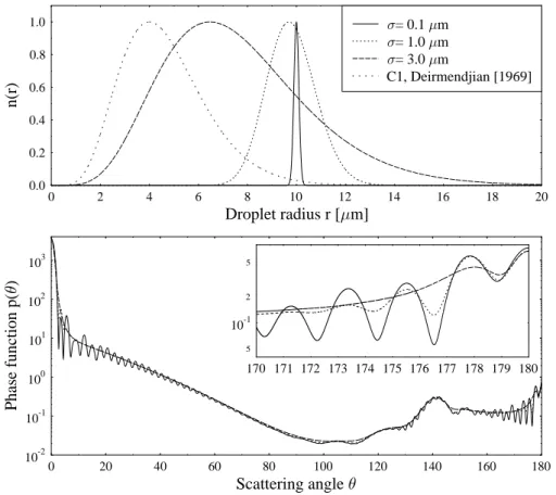
Fig-10

ure1 illustrates this behaviour: Scattering phase functions have been calculated for different size distributions with an identical effective radius of 10 µm using the Mie code ofWiscombe(1980). The corresponding phase functions nearly coincide everywhere, except for some angular regions: These are the backward and forward glories, around 180◦and 0◦scattering angle and the rainbow region, around 140◦ (Laven,2003).

Ob-15

viously, some of the mentioned structures appearing in mono-disperse distributions are not completely smoothed out for narrow size distributions. These features might cause trouble in operational remote sensing methods which are generally based on the assumption of a constant size-distribution. While the shape of the size distribution obviously has only little impact on the single-scattering properties, it is important for the

20

understanding of cloud formation, microphysics, and interaction with aerosol particles. Our results indicate that the size distribution of stratocumulus clouds might actually be much narrower than generally assumed in radiation calculations.

In this study we use exactly those angular regions which might cause problems in usual remote sensing algorithms. Exploiting specific features of the single scattering

25

properties in the 180◦ backward direction, we gain insights into parameters which are not accessible by standard remote sensing techniques, in particular, the width of the

(5)

ACPD

4, 2239–2262, 2004

Full Screen / Esc

Com-pact Airborne Spectrographic Imager (CASI) instrument operated onboard a Do-228 aircraft during the ACE-2 CLOUDYCOLUMN experiment (Brenguier et al.,2000). Sec-tion2briefly describes the CASI instrument and the libRadtran model used in this study and outlines the method. In Sect.3, the technique is illustrated in detail by evaluating

5

a specific observation. In Sect.4the results are summarized and discussed.

2. Methods

2.1. Observations

The Compact Airborne Spectrographic Imager (CASI) (Babey and Anger,1989;Anger et al.,1994) is a “push-broom” imaging spectrometer with a 34◦ field of view across

10

track. The spectral range from 430 nm to 970 nm can be covered with 512 pixels in the spatial axis and 288 spectral channels. During the ACE-2 campaign, CASI was operated onboard the Do-228 aircraft to measure reflected solar radiation. The programmable channels were chosen to allow derivation of cloud albedo and optical thickness (with maximum spatial resolution) as well as cloud top height, using

mea-15

surements within the Oxygen A band over 39 directions. For our study we used the 753 nm channel, with the full angular resolution of 512 pixels, each with 0.07◦ width which translates to a spatial resolution of 2.5 m at cloud top across track. Along track, the resolution is determined by the speed of the aircraft and the sampling time, which evaluates to about 15 m per image pixel. For the quantitative analysis, a moving

aver-20

age over five scan lines along track was applied to the data which effectively reduces the resolution to 75 m along track, keeping the full detail of 2.5 m across track. The uncertainty of the radiance observation is estimated to be about 3%.

The left panel of Fig.2shows an example of a CASI observation where the backscat-ter glory is clearly visible. The measurement was taken on 26 June 1997 for an airmass

25

(6)

ACPD

4, 2239–2262, 2004

Full Screen / Esc

known to frequent air-travellers: From an airplane, the glory is often visible as a bright ring around the aircraft shadow on a cloud. For the pushbroom scanning geometry of the CASI instrument, a cross section through the glory is only visible if (a) the sun is high in the sky (solar zenith angle smaller than 15◦ because otherwise this feature is

5

outside the scanning range of the nadir-looking instrument) and if (b) the flight direction is perpendicular to the solar principal plane (which it is in this case). That the instru-ment is looking exactly in the 180◦backscattering direction is proven by the dark line in the bright center stripe: This is the shadow of the aircraft.

2.2. Simulations

10

For the investigations, extensive Mie calculations were required for various size distri-butions. For the calculations we used the well-tested code byWiscombe (1980). A gamma distribution was assumed as size distribution which is a common assumption in cloud physics:

n(r)= N₀· rµ_{· e}−µ_a0r _, ₍₂₎

15

where a₀is the mode radius, µ defines the shape of the distribution,

N₀= µ

µ+1

Γ(µ + 1)aµ+1

0

(3)

is a normalization constant, andΓ(x) is the gamma function. Probably the most com-mon assumption for a cloud droplet size distribution is the C1 size distribution by Deir-mendjian (1969) which is a gamma distribution with a₀=4 µm and µ=6 (see Fig.1).

20

The effective radius of the gamma distribution evaluates to r_e_ff= R n(r)r 3 dr R n(r)r2_dr = a₀ µ Γ(µ + 4) Γ(µ + 3) (4)

(7)

ACPD

4, 2239–2262, 2004

Full Screen / Esc

devia-tion) is σ= s Z n(r)(r− < r >)2_dr ₌ a0 µ p µ+ 1. (5)

For the C1 byDeirmendjian(1969), r_e_ff=6 µm and σ=1.76 µm.

Various size distributions were sampled, with effective radii r_e_ff between 4 µm and

5

15 µm and widths σ between 0.1 µm and 9 µm. For the calculation of the optical prop-erties by integrating over the size distribution, Mie calculations were carried out with increments of 0.001 µm in the radius range 0.001 to 30 µm.

The scattering phase functions derived from these calculations were used as input to the radiative transfer model libRadtran byKylling and Mayer(1993–2004). libRadtran is

10

a flexible and user-friendly model package to calculate radiance, irradiance, and actinic flux for arbitrary input conditions. The model handles absorption and scattering of molecules and aerosols, as well as water and ice clouds. libRadtran provides a choice of radiative transfer solvers, including the discrete ordinate code DISORT byStamnes et al. (1988) which we used for this study. In particular, version 2.0 of DISORT was

15

used because it is more accurate in handling highly detailed phase functions. To make sure that all details are covered in the necessary angular resolution, the number of streams was set to 256. This high number of streams is essential, since radiances for a narrow angle range are to be calculated which, as our comparisons with less streams show, would be badly sampled and uncertain otherwise.

20

The influence of the atmosphere at 753 nm is very small because this wavelength is outside the important absorption bands. A calculation by libRadtran gives a ver-tically integrated optical thickness due to molecular absorption of only 0.004 for the Midlatitude summer atmosphere ofAnderson et al.(1986), due to some absorption by oxygen, ozone, nitrogen dioxide, and water vapour. The vertically integrated optical

25

thickness of molecular (Rayleigh) scattering is 0.027. The albedo of the underlying water surface is about 0.02, according to the parameterization of sea surface BRDF by

(8)

ACPD

4, 2239–2262, 2004

Full Screen / Esc

Hence, this wavelength is ideally suited for the remote sensing of clouds. For the fol-lowing study, only an isolated cloud layer is considered, neglecting surface albedo and background atmosphere. A test calculation for typical conditions revealed a difference between simulations including and excluding the background atmosphere and surface

5

of less than 0.8% for the upward radiance at the location of the airplane.

The solar zenith angle for the observation to be studied was 10◦, and the scan di-rection was the solar principal plane. Therefore, all following calculations are done for these conditions. Consequently, the 180◦backscatter direction (the center of the glory) corresponds to −10◦in all plots.

10

The middle panel of Fig. 2 shows an example of the libRadtran simulation of the backward glory for four different size distributions. As can be expected from Fig. 1, the glory becomes more prominent for narrow size distributions. As the grey scales for observation and simulation were chosen identically, a mere visual inspection of the images reveals that the width of the size distribution needs to be in the order of 1.0 µm

15

or smaller in order to produce the three center maxima plus three side maxima which are visible in the data. The large µ’s of the gamma-distribution (µ=95 for a width of 1 µm) already indicate that this is much narrower than the widely-used standard C1 cloud model ofDeirmendjian(1969) for which µ=6.

3. Results

20

Our simulations of the reflectivity in the backscatter direction suggested that the shape of the glory is nearly independent of the optical thickness of the cloud, if the latter is larger than about 3. This is demonstrated in Fig.3which shows the “glory reflectivity” R_glory(θ) which we define as

R_glory(θ)= R(θ)− < R(θ) >, (6)

(9)

ACPD

4, 2239–2262, 2004

Full Screen / Esc

< R(θ) >= 1 N N X i=1 R(θ_i) (7)

and N is the number of data points. The curves for optical thickness between 5 and 40 nearly coincide. The reason for this behaviour is easily understood: the glory is a single scattering feature, and if the cloud is optically thick enough to ensure that every

5

photon entering the cloud is scattered at least once, the glory structure should not change anymore. In our case, this is always given since for a cloud of optical thickness 3, a fraction of 1−e−3=0.95 of the photons has undergone at least one scattering. The glory structure sits on top of a multiple-scattering background which of course depends on optical thickness: The bottom plot shows the average reflectivity <R(θ)>,

10

as a function of cloud optical thickness and for various effective radii. The curves show the usual behaviour of the cloud reflectivity outside the glory region. The glory reflectivity R_glory(θ) is therefore a direct measure of the droplet size distribution while the average reflectivity depends mostly on the optical thickness.

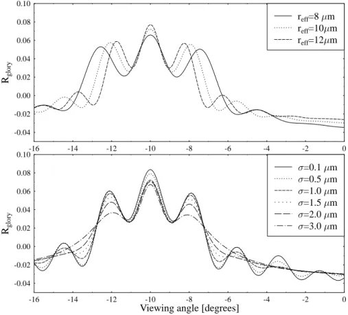
The top panel of Fig.4 shows the glory reflectivity for three different effective radii.

15

The distance of the maxima increases with decreasing droplet size. The bottom panel of Fig.4shows the glory reflectivity R_glory(θ) for an effective radius of 10 µm and dif-ferent widths of the size distribution. Two features are obvious: First, the maxima are more distinguished with decreasing width of the size distribution, as already mentioned. In particular, the side maxima next to the three main maxima are only visible for widths

20

smaller than about 1–1.5 µm. Second, although the shape depends on the width of the size distribution, the distance between neighbouring maxima is almost constant for all investigated cases.

Let us summarize the four most important features of the glory, derived from radiative transfer calculations: First, the average reflectivity in the glory region depends mainly

25

on optical thickness and only little on the droplet size. Second, the shape of the glory does not depend on the optical thickness of the cloud which lead us to the definition

(10)

ACPD

4, 2239–2262, 2004

Full Screen / Esc

effective radius and depends only little on the width of the size distribution. Fourth, the details of the glory reflectivity, in particular the appearance of the side maxima is directly related to the width of the size distribution. Utilizing these four features, a remote sensing scheme for three parameters, optical thickness, effective radius, and

5

width of the size distribution from one single wavelength is developed. We chose a least-square fitting technique, where a function

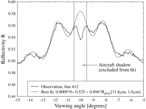
y[r_e_ff, σ](θ)= a · θ + b + c · R_glory[r_e_ff, σ](θ) (8)

is fitted to the data. The third term is the glory, and as the amplitude of the glory reflectivity should only depend on r_e_ff and σ, c would ideally equal 1. However, due to

10

calibration uncertainties, due to small deviations of the viewing direction from the exact 180◦backscatter direction, and due to differences between the actual size distribution from the assumed gamma function, c may deviate from 1 and hence it is a necessary fit parameter.

The second term is basically the average reflectivity and is a function of the optical

15

thickness, see Fig.3. The first term allows some degree of inhomogeneity in the optical thickness, in form of a linear variation of the multiply-scattered radiance within the glory region. This is just an arbitrary assumption and could be replaced by a more complex function – however, one has to make sure that the assumed function does not already fit part of the glory structure which is avoided by the simple linear variation. From a

20

pre-calculated set of functions R_glory for various combinations of r_e_ff and σ the one is chosen which minimizes the cost function

S[r_e_ff, σ]=

N

X

i₌₁

(R(θ_i) − y[r_e_ff, σ](θ_i))2, (9)

where the summation is done over all CASI pixels within ±5◦ of the 180◦ backscatter direction (between −15◦ and −5◦ in the studied case). With this linear least square

25

(11)

ACPD

4, 2239–2262, 2004

Full Screen / Esc

ex-ample of such a fit is shown in Fig. 5. Scan line 612 was extracted from the CASI observation (see dotted line in Fig.2) because the cloud seems to be reasonably ho-mogeneous in this region. The thick line is the observation, with the aircraft shadow clearly visible in the center. The marked region has been excluded from the fit. The

5

thin line is the best fit.

The glory itself and the first side maximum is almost perfectly fitted by the simulated glory reflectivity for effective radius 11.8 µm and width 1 µm. The scaling factor is reasonably close to 1 (0.896). The multiple scattering background is described by the first two terms; the linear variation is negligible in this case. The background can

10

be used to determine the optical thickness, according to Fig. 3: Using the curve for r_e_ff=11.8µm, an optical thickness of 13.2 is determined.

To automate the algorithm, another step is neccessary. As Fig.2shows, the location of the glory varies slightly in the image which is due to the changing aircraft attitude with respect to the nadir direction and the solar principle plane. The available data for

15

pitch, roll, and yaw of the aircraft were not accurate enough to correct the image with the desired accuracy of one CASI pixel (0.07◦). Therefore, a simple edge detection technique was applied to the image, to automatically identify the aircraft shadow and to align the image correspondingly, see Appendix.

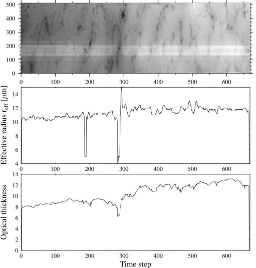
The top panel of Fig. 6 shows the stratified CASI observation, after application of

20

the described algorithm. The aircraft motion is completely corrected, and the glory is transformed to a straight line. The lower two plots show the results for the optical thick-ness and effective radius. The effective radius shows surprisingly little noise, except for regions where large inhomogeneities occur around the 180◦ backscatter direction. The effective radius is rather smooth in particular in the left part of the image where

25

the cloud inhomogeneity is small. The effective radius is between 10 and 12 µm which is reasonable for this type of boundary layer cloud. The optical thickness is also in the expected range.

(12)

ACPD

4, 2239–2262, 2004

Full Screen / Esc

out to be not very robust. This is immediately obvious from Fig.4: The information about the width of the size distribution is hidden in small details, e.g. the appearance of the side maxima which in this example vanishes for widths larger than 1.5 µm. These small details, however, are easily shadowed by the natural variability of the signal and it

5

is clear that the width of the size distribution cannot be derived from a single scan line. Therefore, the following averaging procedure was chosen: First, the effective radius was determined as in Fig.6, assuming a constant width of 1 µm (the assumption of a constant width has only little impact on the derived effective radius); second, scan lines with identical effective radii were averaged (in bins of width 0.2 µm). This sorting by

10

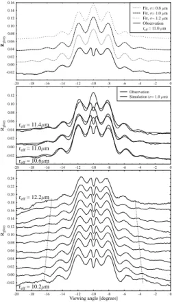
effective radius reduces the influence of cloud inhomogeneity considerably. Figure7 shows an exemplary outcome of this procedure.

The top panel presents the averaged reflectivity for effective radius 11 µm (thick line) which is an average over 50 individual scan lines. In contrast to a single scan line (Fig.5), the noise is reduced considerably and two secondary maxima at each side of

15

the three main maxima are clearly distinguishable. In comparison to the experimen-tal data (thick line), three fit curves (according to Eq. 8) for different widths 0.8 µm, 1.0 µm, and 1.2 µm (dotted lines) are presented. Visual comparision of the side max-ima suggests a width of 1.0 µm. For 1.2 µm the second side maximum, which is clearly visible in the observation, is hardly distinguishable in the simulation. The middle panel

20

shows the results for effective radii 10.6 µm, 11.0 µm, and 11.4 µm, in direct compar-ison with the best fit model curves. Finally, the bottom plot presents averages for 11 effective radii between 10.2 µm and 12.2 µm (all curves are shown for which more than 10 scan lines were available to calculate the average). For each individual curve, the second side-maxima are clearly distinguishable. The dotted line mark the location of

25

the second side maximum according to the simulation. In some cases, even the third side-maxima are visible. From all this evidence it can be concluded that the width of the size distribution is about 1.0 µm for this observation. As the figure illustrates, for widths larger than about 1.2 µm the second side-maximum vanishes, while for widths smaller

(13)

ACPD

4, 2239–2262, 2004

Full Screen / Esc

observation.

4. Conclusions

Based on spatial high resolution observations, a retrieval scheme is presented which allows the simultaneous determination of optical thickness, effective radius and the

5

width of the droplet size distribution from observations at one single wavelength. The retrieval relies on the observation of the glory in the 180◦ backscatter direction at 753 nm. It has been shown by combined Mie calculations and radiative transfer simula-tions, that the effect of an increasing optical thickness increases the average reflectivity but does not affect the characteristic appearance of the glory. The glory itself depends

10

on the effective radius and the width of the droplet size distribution. While the distance of the maxima is basically a function of the effective radius, the amplitude of the smaller side maxima is determined by the width of the droplet size distribution. In particular, for an effective radius of about 10 µm, the secondary maxima are only distinguishable if the width of the size distribution is about 1 µm or smaller. As this is the case in the

15

example studied here and also in many other observations during this campaign, we conclude that the width of the size distribution was about 1 µm which is considerably smaller than what is often assumed for radiation calculations, see Fig. 1. Simulta-neous microphysical measurements and theoretical considerations during the ACE-2 CLOUDYCOLUMN campaign confirm the existence of narrow droplet distributions. In

20

particular, Fig. 2 fromSch ¨uller et al.(2003) shows a measured droplet spectrum which is very close to the 1 µm curve in Fig.1.

Special features like the rainbow or the glory have been previously exploited for the study of cloud properties. Spinhirne and Nakajima (1994) suggested to use aircraft observations of the glory for remote sensing of droplet sizes. In particular they

recom-25

mended to use near-infrared observations where the multiple-scattering background is suppressed due to absorption in water droplets. Breon and Goloub(1998) followed a

(14)

ACPD

4, 2239–2262, 2004

Full Screen / Esc

used three spectral channels in the visible and utilized POLDER’s ability to measure polarized radiances. With this method they were able to retrieve the effective radius in a field of view between 150◦ and 170◦. They exploit a similar sensitivity of the po-larized phase function to effective radius and the width of the droplet size distribution.

5

For practical application it has to be kept in mind that the method requires reasonably homogeneous cloud conditions over the required angular range. A variability of optical thickness or effective radius blurs the specific features of the glory, see also ( Rosen-feld and Feingold,2003). In the case of the CASI observation where the aircraft flight altitude was about 2 km above the cloud, the 10◦ which were used for the evaluation

10

translate to only 350 m over which homogeneity is required. In the case of the low-Earth-orbiting Polder, however, the angular range used in the analysis corresponded to about 150 km (Breon and Goloub,1998). It is immediately obvious that the homogene-ity criterion is much easier fulfilled for a low-flying aircraft. In fact, the flight altitude of 2 km above the cloud of the Do-228 in this paper is ideal for this application: a lower

15

flight altitude is desirable to minimize cloud inhomogeneity within the required angular range. On the other hand, a lower flight altitude would cause the aircraft shadow to cover a larger angular range which would prevent a quantitative analysis (see Fig.5).

The retrieval of optical thickness and effective radius proved to be robust while the width of the size distribution strongly depends on features of small intensity, in particular

20

on the side maxima of the glory. Therefore, averaging scan lines with similar effective radii is essential for the determination of the width of the distribution and improves the quality significantly. For future cloud physics campaigns, such measurements should be considered a valuable addition, if the sun is high enough to permit a high-resolution observation of the glory. In case studies, this approach can build a powerful link

be-25

tween microphysical and radiation measurements. For such studies, the scan direction must exactly cross through the 180◦backscatter direction. A small mis-alignment would cause large problems in the evaluation of the data. The quality of the alignment can be easily determined from the visibility of the aircraft shadow in the data.

(15)

ACPD

4, 2239–2262, 2004

Full Screen / Esc

a single scattering phenomenon, it is not affected by three-dimensional cloud inhomo-geneity effects. Generally, reflected radiance is clearly affected by cloud inhomogeneity and net horizontal photon transport which causes radiative smoothing (Marshak et al., 1995). Hence, the derived optical thickness is artificially smoothed over a scale

deter-5

mined by the physical cloud height. This is also true for the optical thickness derived by our method. Properties derived from single-scattered glory reflectivity (effective radius and width of the size distribution), on the other hand, are not affected by smoothing and are hence representative for the area used in the retrieval; in our case, 350 m×75 m.

From the occurrence of the side maxima, we concluded that the width of the droplet

10

size distribution was about 1µm or less for the marine stratocumulus during the ACE-2 CLOUDYCOLUMN experiment. Such a distribution looks conceptually different to what is generally used in radiation studies, see Fig.1. The top panel shows the commonly employed C1 size distribution byDeirmendjian (1969) in comparison to a size distri-bution which is more representative of the conditions observed here, in particular, the

15

curve for effective radius 10 µm and width 1 µm. Simultaneous microphysical measure-ments and theoretical considerations during the ACE-2 CLOUDYCOLUMN campaign confirm the existence of narrow droplet distributions (Sch ¨uller et al.,2003).

Appendix: Image alignment

To correct the image for aircraft misalignment we developed a technique which

auto-20

matically identifies the position of the aircraft shadow. As Fig. 5 shows, the aircraft shadow is the region with the strongest gradient in the image. The Sobel edge detec-tion algorithm (see e.g.Cherri and Karim,1989) was chosen to identify the strongest

(16)

ACPD

4, 2239–2262, 2004

Full Screen / Esc

  −1 0+1 −2 0+2 −1 0+1   (10)

which is similar to a derivative. The result is large when the gradient perpendicular to the flight track is large. Numbers smaller than zero indicate negative gradients, num-bers larger than 0 positive ones. For the presented example the minima and maxima

5

of the convolved image marked the left and right side of the aircraft shadow in more than 75% of all scan lines. Cloud edges which are present in several parts of the im-age, may cause problems with this method. Therefore, we introduced the following two extra requirements: (1) maximum and minimum gradient are required to lie within certain bounds; a histogram of distances between minimum and maximum is created,

10

and all data points are excluded where this distance deviates by more than 2 pixels from the histogram maximum; this way, the width of the aircraft shadow is determined dynamically for the image; (2) for all the scan lines that fulfil the first criterion, the 180◦ backscatter direction is assumed to lie midway between the minimum and maximum gradients; from this set of data points those are excluded which deviate by more than a

15

certain threshold from the linear interpolation between the adjacent scan lines; for the example in Fig.2 this threshold was set to 1 pixel. Finally, the gaps are filled by lin-ear interpolation between the thus determined points. Although these criterions seem rather strict, 506 out of 668 scan lines remained to determine the location of the 180◦ backscatter direction. The result is shown in Fig.6which clearly illustrates the potential

20

of the method.

Acknowledgements. M. Schr ¨oder was supported by the German BMBF project 4D-Clouds un-der contract number 07ATF24.

(17)

ACPD

4, 2239–2262, 2004

Full Screen / Esc

References

Anderson, G., Clough, S., Kneizys, F., Chetwynd, J., and Shettle, E.: AFGL Atmospheric Con-stituent Profiles (0–120 km), Tech. Rep. AFGL-TR-86-0110, AFGL (OPI), Hanscom AFB, MA 01736, 1986. 2244

Anger, C., Mah, S., and Babey, S.: Technological enhancements to the Compact Airborne

5

Spectrographic Imager (casi), in Proceedings of the Second International Airborne Remote Sensing Conference and Exhibition, 12–15 September, Strasbourg, France, pp. 205–214, 1994. 2242

Babey, S. and Anger, C.: A compact airborne spectrographic imager (casi), in Proceedings of IGARSS, IEEE, Vancouver, vol. 2, pp. 1028–1031, 1989. 2242

10

Brenguier, J., Chuang, P., Fouquart, Y., Johnson, D., Parol, F., Pawlowska, H., Pelon, J., Sch ¨uller, L., Schr ¨oder, F., and Snider, J.: An overview of the ACE-2 CLOUDYCOLUMN closure experiment, Tellus B, 52, 815–827, 2000. 2242

Breon, F.-M. and Goloub, P.: Cloud droplet effective radius from spaceborne polarization mea-surements, Geophys. Res. Lett., 25, 1879–1882, 1998. 2250,2251

15

Cherri, A. and Karim, M.: Optical symbolic substitution: edge detection using Prewitt, Sobel, and Roberts operators, Applied Optics, 28, 4644–4648, 1989. 2252

Cox, C. and Munk, W.: Measurement of the roughness of the sea surface from photographs of the sun’s glitter, Journal of the Optical Society of America, 44, 838–850, 1954. 2245

Deirmendjian, D.: Electromagnetic Scattering on Spherical Polydispersions, American Elsevier

20

Publishing Company, Inc., New York, 1969. 2243,2244,2245,2252,2256

Hansen, J. and Pollack, J.: Near-infrared light scattering by terrestrial clouds, J. Atmos. Sci., 27, 265–281, 1970. 2241

Houghton, J., Ding, Y., Griggs, D., Noguer, M., van der Linden, P., Dai, X., Maskell, K., and Johnson, C.: Climate change 2001: The scientific basis, Tech. rep., Intergovernmental

25

Panel on Climate Change (IPCC), IPCC Secretariat, c/o World Meteorological Organization, Geneva, Switzerland, 2001. 2240

Kylling, A. and Mayer, B.: Libradtran, a package for radiative transfer calculations in the ultravi-olet, visible, and infrared,http://www.libradtran.org, 1993–2004. 2244

Laven, P.: Simulation of rainbows, coronas, and glories by use of Mie theory, Applied Optics,

30

42, 436–444, 2003. 2241

(18)

ACPD

4, 2239–2262, 2004

Full Screen / Esc

Nakajima, T. and Tanaka, M.: Effect of wind-generated waves on the transfer of solar radiation in the atmosphere-ocean system, J. Quant. Spectrosc. Radiat. Transfer, 29, 521–537, 1983.

2245

Rosenfeld, D. and Feingold, G.: Explanations of discrepancies among satellite observations

5

of the aerosol indirect effects, Geophys. Res. Lett., 30, doi:10.1029/2003GL017684, 2003.

2251

Sch ¨uller, L., Brenguier, J.-L., and Pawlowska, H.: Retrieval of microphysical, geometrical, and radiative properties of marine stratocumulus from remote sensing, J. Geophys. Res., 108, doi:10.1029/2002JD002680, 2003. 2250,2252

10

Spinhirne, J. and Nakajima, T.: Glory of clouds in the near infrared, Applied Optics, 33, 4652– 4662, 1994. 2250

Stamnes, K., Tsay, S., Wiscombe, W., and Jayaweera, K.: A numerically stable algorithm for discrete-ordinate-method radiative transfer in multiple scattering and emitting layered media, Applied Optics, 27, 2502–2509, 1988. 2244

Wiscombe, W.: Improved Mie scattering algorithms, Applied Optics, 19, 1505–1509, 1980.

(19)

ACPD

4, 2239–2262, 2004

Full Screen / Esc

Print Version Interactive Discussion © EGU 2004 0 2 4 6 8 10 12 14 16 18 20 Droplet radius r [ m] 0.0 0.2 0.4 0.6 0.8 1.0 n(r) C1, Deirmendjian [1969] = 3.0 m = 1.0 m = 0.1 m 0 20 40 60 80 100 120 140 160 180 Scattering angle 10-2 10-1 100 101 102 103 Phase function p( ) 170 171 172 173 174 175 176 177 178 179 180 5 10-1 2 5

Fig. 1. (Top) Gamma droplet size distributions with different widths but identical effective radius

10 µm; the C1 size distribution byDeirmendjian(1969) is also shown for comparison. (Bottom) Scattering phase functions for the three size distributions with effective radius 10 µm; the small graph shows a zoom into the 180◦backscatter direction.

(20)

ACPD

4, 2239–2262, 2004

Full Screen / Esc

Print Version Interactive Discussion © EGU 2004 0 2 4 6 8 10 12 14 16 18 20 = 5.5 = 3.0 m 0 2 4 6 8 10 12 14 16 18 20 = 19.8 = 2.0 m 0 2 4 6 8 10 12 14 16 18 20 = 95 = 1.0 m 0 2 4 6 8 10 12 14 16 18 20 Droplet radius [ m] = 395 = 0.5 m

Fig. 2. CASI observation for 26 June 1997 (left); the length of the flight leg is 10 km and the

width of the strip is 1.2 km at cloud top. Simulated reflectivity distribution on the same angular grid (middle) for four different droplet size distributions (right) with identical effective radius 10 µm. The dotted line marks scan line 612 which will be studied in more detail later.

(21)

ACPD

4, 2239–2262, 2004

Full Screen / Esc

-16 -14 -12 -10 -8 -6 -4 -2 0

Viewing angle [degrees]

-0.04 -0.02 0.00 0.02 0.04 0.06 0.08 0.10 Rglory = R( ) -<R( )> =40 =30 =20 =15 =10 =5 0 5 10 15 20 25 30 35 40 45 50 Optical thickness 0.0 0.1 0.2 0.3 0.4 0.5 0.6 0.7 0.8 0.9 1.0 A verage reflectivity <R( )> reff= 12.0 m reff= 10.0 m reff= 8.0 m reff= 6.0 m reff= 4.0 m

Fig. 3. (Top) Glory reflectivity, after subtraction of the average, see Eq. (6), for effective ra-dius 10 µm and width 1 µm. (Bottom) Average reflectivity in the 180◦backscatter direction, as function of the optical thickness.

(22)

ACPD

4, 2239–2262, 2004

Full Screen / Esc

Print Version Interactive Discussion © EGU 2004 -16 -14 -12 -10 -8 -6 -4 -2 0 -0.04 -0.02 0.00 0.02 0.04 0.06 0.08 0.10 Rglory reff=12 m reff=10 m reff=8 m -16 -14 -12 -10 -8 -6 -4 -2 0

-0.04 -0.02 0.00 0.02 0.04 0.06 0.08 0.10 Rglory =3.0 m =2.0 m =1.5 m =1.0 m =0.5 m =0.1 m

Fig. 4. (Top) The glory reflectivity for three different effective radii but constant width 1 µm.

(Bottom) The glory as a function of the width of the size distribution for indentical effective radius 10 µm.

(23)

ACPD

4, 2239–2262, 2004

Full Screen / Esc

-15 -14 -13 -12 -11 -10 -9 -8 -7 -6 -5

Viewing angle [degrees]

0.44 0.46 0.48 0.50 0.52 0.54 0.56 0.58 0.60

Reflectivity

R

Best fit, 0.0009* + 0.525 + 0.896*Rglory[11.8 m, 1.0 m]

Observation, line 612

Aircraft shadow (excluded from fit)

Fig. 5. Example of a fit for scan line 612; the thick line is the observed reflectivity and the thin

line is the best fit. The width of the aircraft shadow is about 8 pixel or 20 m which is close to the actual wing-span of the Do-228 of 17 m.

(24)

ACPD

4, 2239–2262, 2004

Full Screen / Esc

Print Version Interactive Discussion © EGU 2004 0 100 200 300 400 500 600 0 100 200 300 400 500 0 100 200 300 400 500 600 4 6 8 10 12 14 Ef fective radius reff [ m] 0 100 200 300 400 500 600 Time step 0 2 4 6 8 10 12 14 Optical thickness

Fig. 6. (Top) Stratified CASI observation; (middle) retrieved effective radius (µm); (bottom)

(25)

ACPD

4, 2239–2262, 2004

Full Screen / Esc

Print Version Interactive Discussion © EGU 2004 -20 -18 -16 -14 -12 -10 -8 -6 -4 -2 0 -0.02 0.00 0.02 0.04 0.06 0.08 0.10 0.12 0.14 0.16 Rglory reff= 11.0 m Observation Fit, = 1.2 m Fit, = 1.0 m Fit, = 0.8 m -20 -18 -16 -14 -12 -10 -8 -6 -4 -2 0 -0.02 0.00 0.02 0.04 0.06 0.08 0.10 0.12 Rglory Simulation ( = 1.0 m) Observation -20 -18 -16 -14 -12 -10 -8 -6 -4 -2 0

-0.02 0.00 0.02 0.04 0.06 0.08 0.10 0.12 0.14 0.16 0.18 0.20 0.22 0.24 Rglory reff= 10.6 m reff= 11.0 m reff= 11.4 m reff= 10.2 m reff= 12.2 m

Fig. 7. (Top) Glory reflectivity, average over all scan lines with effective radius 11 µm (thick

line) and simulated glory reflectivities for three different widths of the size distribution, shifted by a constant amount; (middle) same for three effective radii 10.6 µm, 11.0 µm, and 11.4 µm, in comparison with the model fit for width 1 µm; (bottom) averages for all effective radii where more than 10 scan lines were available; the dashed curves indicate the location of the second side-maximum according to the simulation of the glory.