The development of steady State and lifetime fluorescence instruments for real time in situ aquatic chemistry measurements

The Development of Steady State and Lifetime Fluorescence Instruments for Real Time In Situ Aquatic Chemistry Measurements

by

Schuyler Senft-Grupp

S.B., Massachusetts Institute of Technology (2006)

MGHou

MASSACHUSETTS INSTITUTE

OF TECHNOLOLGY

MAY 052015

LIBRARIES

Submitted to the Department of Civil and Environmental Engineering in Partial Fulfillment of the Requirements for the Degree of

Doctor of Philosophy at the

MASSACHUSETTS INSTITUTE OF TECHNOLOGY

February 2015

2015 Massachusetts Institute of Technology. All rights reserved

Signature redacted

Signature of Author...

'9

...

12epartment of ivil and Environmental Engineering January 29, 2015

Signature redacted

C ertified b y ... ...

Harold F. Hemond William E. Leonhard Professor of Civil and Environmental Engineering

Signature redacted

A ccepted by... ...

Heidi Nepf Donald and Martha Harleman Professor of Ci il and Environmental Engineering

MITLibraries

77 Massachusetts Avenue Cambridge, MA 02139 http://Iibraries.mit.edu/ask

DISCLAIMER NOTICE

Due to the condition of the original material, there are unavoidable flaws in this reproduction. We have made every effort possible to provide you with the best copy available.

Thank you.

The images contained in this document are of the best quality available.

The Development of Steady State and Lifetime Fluorescence Instruments for Real Time In Situ Aquatic Chemistry Measurements

by

Schuyler Senft-Grupp

Submitted to the Department of Civil and Environmental Engineering on January 29, 2015 in Partial Fulfillment of the

Requirements for the Degree of Doctor of Philosophy in Environmental Engineering and Instrumentation

ABSTRACT

The development of three optical instruments for the chemical exploration and

characterization of natural waters is described. The first instrument (called LEDIF) employs a novel flowcell, 6 UV LEDs as excitation sources, a wideband lamp, and a spectrometer to measure steady state chemical fluorescence and absorbance. The instrument is packaged aboard an autonomous underwater vehicle (AUV) and demonstrates the ability to map chemical

concentrations in three dimensions. The second instrument repackages the sensor components to study dissolved organic matter (DOM) in tropical Southeast Asia peatland rainforests. This instrument is optimized for low power consumption over long deployments to remote locations. Two field trials in Pontianak Indonesia with durations of two and six weeks captured peatland river fluorescence measurements at 20 minute intervals. The results show changes in DOM linked to tidally induced water level fluctuations and provide insight into the complex biogeochemical dynamics of the system.

The third instrument increases the chemical sensitivity and specificity of LEDIF with the addition of fluorescence lifetime sensing capabilities. The development of this sensor for AUV deployment required the engineering of a compact, low power, high speed (GHz) data

acquisition circuit board. The resulting circuit digitizes data at a rate of 1 gigasample/second and performs user customizable digital signal processing. This board is used along with a 266 nm

concentration pyrene to demonstrate its ability to identify small, long-lived fluorescence signals in the presence of large background fluorescence. Results indicate a pyrene limit of detection below environmentally relevant levels. The final overall instrument dimensions allows it to be packaged for future AUV deployments.

Thesis Supervisor: Harold F. Hemond

Table of Contents

Acknowledgements 15

Chapter 1 Introduction 17

1.1 Understanding Our Environment: Personal Motivation 17 1.2 The Case for Real Time In Situ Aquatic Chemistry Sensing 17

1.2.1 Chemical Heterogeneity Exists in Water Bodies 18

1.2.2 Identifying Chemical Contamination Sources 18

1.2.3 Increased Data

Quality

1.2.4 Rapid Emergency Response and Contamination Delineation 19

1.2.5 New Aquatic Sensing Platforms Require New Sensors 19

1.3 Optical Sensing 20

1.4 Development of New Fluorescence Instruments for In Situ Applications 20

1.5 References 21

Chapter 2 A Multi-Platform Optical Sensor for In Situ Sensing of Water Chemistry _ 23

2.1 Introduction 24

2.2 Materials and Procedures 26

2.2.1 Sensor Module Overview 26

2.2.2 Flowcell geometry 27

2.2.3 Excitation-Emission Optical System 27

2.2.4 Power Control Board 28

2.2.5 Computer 28

2.2.6 Software 29

2.2.7 Spectrometer 29

2.2.8 Sample Flow 30

2.3 Assessment 30

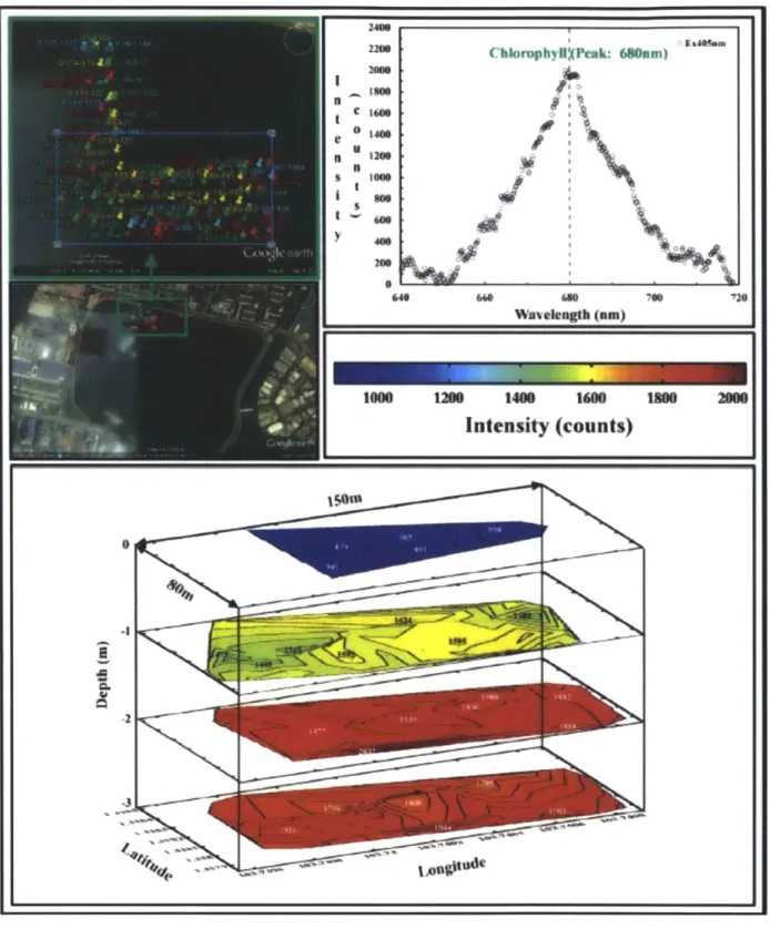
2.3.1 Fluorescence Peak Validation 31

2.3.2 Field Samples Comparison 31

2.3.3 Multi-spectral and EEM Demonstration 32

2.3.4 Absorbance Measurement 32

2.3.5 Turbidity Measurement 33

2.3.6 Pressure and Temperature Effects 33

2.3.7 Field Deployment 34

2.4 Discussion 34

2.5 Comments and Recommendations 35

2.7 References

2.8 Figures and Tables 39

Chapter 3 An In Situ Spectrophotometer and Fluorometer for River DOM

Characterization in Peatland Rainforests 47

3.1 Introduction ₄₇

3.2 Measuring in situ DOC via Fluorescence 48

3.3 Instrument Description 49

3.3.1 Optical Configuration 50

3.3.2 Control Circuit Board 50

3.3.3 Fluorescence LED Excitation Sources 51

3.3.4 Wideband Absorbance Lamp 52

3.3.5 Spectrometer 52

3.3.6 Batteries 52

3.3.7 Pressure Housing 53

3.3.8 Instrument Measurement Procedure 53

3.4 Methods 55

3.4.1 Laboratory Testing With River Water 55

3.4.2 River Deployment 55

3.4.3 Optical Absorbance/Fluorescence Simulation 56

3.5 Results 59

3.5.1 Simulation 59

3.5.2 River Water Dilution 60

3.5.3 River Deployment 61

3.6 Discussion 62

3.6.1 Field Data Interpretation 62

3.6.2 Inverse Fluorescence Response 63

3.6.3 Absorbance Measurements 63

3.6.4 Fluorescence Peak Shift 63

3.6.5 Calibrating For Concentration and Turbidity 64

3.6.6 Estimating Changes in DOC 64

3.7 Conclusion 65

3.8 Acknowledgements 66

3.9 References 66

3.10 Figures 68

Chapter 4 Gigahertz Data Acquisition System for Embedded Sensors 79

4.2 Data Acquisition System Description 80

4.2.1 Analog-to-Digital Conversion 81

4.2.2 Data Capture and Storage 82

4.2.3 High Speed Trigger 82

4.2.4 Power Management System 83

4.2.5 External Communication 84

4.2.6 Printed Circuit Board 84

4.3 Circuit Operation 84

4.3.1 Power On and Initialization of FPGA 85

4.3.2 Power On and Initialization of ADC 85

4.3.3 Data Acquisition 85

4.3.4 Additional System Features 87

4.4 Test methods 87

4.5 Results 88

4.5.1 Analog-to-Digital Conversion 88

4.5.2 Power Consumption 89

4.5.3 Design and Cost 89

4.6 Discussion 89

4.6.1 Applications 89

4.6.2 FPGA and Digital Signal Processing 90

4.6.3 Future Work 90

4.7 Conclusion 91

4.8 Acknowledgements 91

4.9 References 91

4.10 Figures and Tables 93

Chapter 5 A Compact Fluorescence Lifetime Instrument for In Situ Investigation of

PAHs 106

5.1 Introduction 106

5.1.1 Overview 106

5.1.2 PAHs in the Environment 107

5.1.3 Fluorescence and Fluorescence Lifetime Theory 108

5.1.4 Pyrene Fluorescence 109

5.1.5 AUV In Situ Fluorescence Research (LEDIF) 109

5.1.6 Previous In Situ Instruments for the Study of PAHs in Natural Waters 110

5.1.7 High Speed Data Acquisition 110

5.1.8 Research Objective

5.2 Fluorescence Lifetime Instrument Design 5.2.1 Instrument Overview

5.2.2 Instrument Components 5.2.3 Signal Processing

5.2.4 Instrument Operation Procedure_

5.3 Test Method

5.3.1 Instrument Setup 5.3.2 Sample Preparation 5.3.3 Experiments

5.4 Results and Discussion 5.4.1 Pyrene Quantification 5.4.2 Full Spectrum Scans 5.4.3 Power and Size

5.5 Conclusion

5.6 Acknowledgments 5.7 References

5.8 Figures

Chapter 6 Conclusion

Appendix A Validating LEDIF Field Performance.

A.1 Chlorophyll a Calibration A.2 Field Results

A.3 References

Appendix B Spectral Intensity Distributions for LI B.1 260 nm LED B.2 285 nm LED B.3 315 nm LED _ B.4 340 nm LED_ B.5 370 nm LED B.6 390 nm LED B.7 405 nm LED_ B.8 430 nm LED

DIF and DOM Instrument LE

110 111 111 _ 112 113 116 117 117 117 _117 118 118 _118 119 __ 119 __ 121 121 123 128 131 131 132 132 Ds 133 133 134 134 135 135 136 136 137

Appendix C Monte Carlo Photon Absorbance and Fluorescence Simulation 138

Appendix D DOM Instrument Microcontroller Code 145

D.lMain

D. 1.1 Header File 145

D. 1.2 Main Code and Helper Functions 147

D.2 Real Time Clock (RTC) Library 161

D.2.1 Header File 161

D.2.2 RTC Library Code 162

D.3 LED Driver Library 164

D.3.1 Header File 164

D.3.2 LED Driver Main Code 165

List of Figures

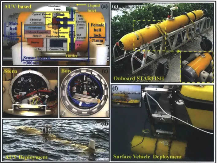
Figure 2.1 The layout of LEDIF and the demonstration of its multi-platform deployment

capability: (a, b, and c) Front, stern, and bow views of LEDIF packaged inside the pressure hull,

(d) LEDIF aboard STARFISH deployed in the field for sensing of water chemistry, (e) LEDIF

integrated to the STARFISH, and (f) LEDIF is end capped for surface vehicles deployment,

utilizing a simple interface box for communication and external brackets. 40

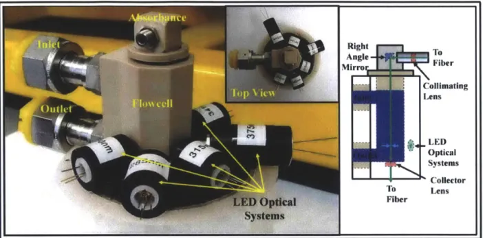
Figure 2.2 LEDIF multi-excitation optical flowcell system. 41

Figure 2.3 Block diagram of LEDIF power control board. 41

Figure 2.4 3-D transient modeling of through hull flow transportation manifold: (a) Liquid

chamber of the through hull flow transportation manifold, (b) Particle pathlines coloured by elapsed time (s) at 100 m depth, 3 knots transverse velocity, (c) Flow retention time at various

operating conditions, and Internal velocity contours (m/s) of (d) typical (0.21 million cells) and

(e) high density (1.05 million cells) mesh at 100 m depth, 3 knots transverse velocity. 42

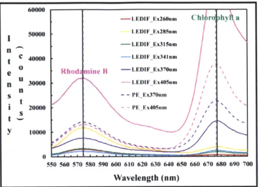
Figure 2.5 Emission peaks comparison between LEDIF and Perkin Elmer LS-55 of a lab

mixture (normalized by a factor equal to -63.5). Note: Symbol legend in instrument excitation

wavelength format. 43

Figure 2.6 Emission spectra from Brunei peatland water samples at various depths, observed

using LEDIF and Perkin Elmer LS-55 (normalized by a factor equal to -8). This shift can be attributed to the longer excitation wavelength and the wavelength dependent response of the

USB4000 compared to the PE LS-55. 43

Figure 2.7 Emission spectrum and excitation-emission matrix of a complex lab mixture. The

table lists the observed and reference fluorescence emission values. 44

Figure 2.8 The absorbance of rhodamine B (dissolved in water) measured by LEDIF and

compared with PhotoChemCAD: (a) At various concentrations, and (b) For low concentration sample, absorbance as low as 0.01 can be accurately measured. 44

Figure 2.9 Linear calibration curve for turbidity measurement of LEDIF: (a) Measurement of

excitation light scattering of known turbidity standards, (b) Turbidity below 1 NTU (typical requirement by water authorities) can be measured for the application of screening processed water, and (c) Scattering of the excitation intensity can be calibrated and described with a single

correlation for the turbidity (NTU) measurement. 45

Figure 2.10 3D subsurface mapping of chlorophyll a concentration performed with LEDIF

aboard STARFISH in the late morning of 20th December 2011 at Pandan reservoir, Singapore. The measurements demonstrated the successful operation of LEDIF in the freshwater

environment for 3D subsurface mapping. 46

Figure 3.1 System Overview. 68

Figure 3.2 Optical Component Orientation. Instrument optical component layout consisting of a)

a fluorescence excitation LED; b) light collection fiber optic cable connected to spectrometer; c) fused silica optical window; d) fiber optic cable connected to wide spectrum lamp for

created by a and d, and the cone of acceptance for b. Since a and b are in the same plane looking

out the same direction, they are considered to be at 0 degrees orientation. 68 Figure 3.3 Instrument Configuration and Optics. Top: Side view of the initial prototype of the

instrument optical components. Bottom: Front view of the instrument face for the final deployed instrument. The absorbance source arm was modified and painted black to reduce its

reflectiveness. 69

Figure 3.4 Control Circuit Board. 70

Figure 3.5 LED Circuit Board. The PCB is populated with five excitation LEDs and has an

opening for the collection fiber optic. The LED controller IC and wire connector are located on

the back of the PCB. 70

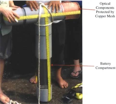
Figure 3.6 Instrument Housing. The instrument, shown prior to deployment, is held together

with ratcheting straps. 71

Figure 3.7 Deployment Location. The instrument was secured to a jetty located in front of the

red building, downstream from the river convergence. River flow is from right to left 71 Figure 3.8 Comparison of Simulation, Instrument, and Lab Fluorescence Spectra. The

instrument spectra have been scaled to the simulation data to better illustrate shape and

wavelength range. 72

Figure 3.9 Simulation Results for Increasing DOM Concentrations. 72

Figure 3.10 River Fluorescence Measured with Instrument. Each line represents the fluorescence

with a different excitation wavelength. 73

Figure 3.11 River Fluorescence Measured with Lab Fluorometer. 73 Figure 3.12 River Absorbance Spectrum Measured with Lab Spectrophotometer. 74

Figure 3.13 River Dilution Fluorescence Test #1. This figure shows the results of the first river

water dilution test with excitation at 375nm. Each line represents a different DOM concentration and turbidity. The turbidity values shown in the legend represent the percent turbidity relative to the initial sample. Lower DOM and lower turbidity are correlated with greater fluorescence. _ 74 Figure 3.14 River Dilution Fluorescence Test #2. This figure shows the results of the second

river water dilution test with excitation at 375nm. 75

Figure 3.15 Fluorescence Response as Function of DOM. This figure shows the cumulative

measured fluorescence for the dilution tests as a function of DOC. In the regions marked a and b,

the change in fluorescence is due to changing turbidity. 75

Figure 3.16 Fluorescence Response as Function of Turbidity. This figure shows the cumulative

measured fluorescence for the dilution tests as a function of turbidity. In the regions marked a and b, turbidity is changing but DOM concentration is constant. 76 Figure 3.17 Instrument Battery Voltage. The battery exceeded its specified lifetime of four

weeks. Even with the eventual significant decrease in voltage the instrument was able to keep

operating down to 32 V. 76

Figure 3.18 River Deployment #1. Fluorescence peak values for two excitations are plotted

Figure 3.19 River Deployment #2. Fluorescence peak values for two excitations are plotted

along with river depth. Higher fluorescence indicates lower DOM and/or turbidity. The instrument experienced conditions around 2/27 that impaired its measurement ability for the

remainder of the deployment by covering the optical window in silt. 77 Figure 3.21 Comparison between TOC Analyzer and Instrument. The samples were gathered

over a 6 hour period on February 2"d. 78 Figure 3.22 Estimates of DOC concentrations assuming constant turbidity. 78

Figure 4.1 Data acquisition board as part of an instrument. 94

Figure 4.2 Data acquisition circuit sub-system diagram. 94

Figure 4.3 Photo of populated circuit board. 95

Figure 4.4 PCB 4 Layer Stack Up. The 4-layer board stack up is standard and available through

most PCB printing companies [15]. Units are mil (thousands of an inch). 95

Figure 4.5 Trigger Circuit Schematic 96

Figure 4.6 Simplified diagram of FPGA for basic data acquisition. The trigger signal feeds a

state machine that asserts the Write Enable signal of the FIFO until it is full. The UART state machine controls the Read Enable signal and asserts this whenever it is ready to send the next byte of data and the FIFO is not empty. The FIFO is automatically generated by the Xilinx ISE and handles cross clock domain logic and asymmetrical data write and read widths. Additionally the user can programmatically set the FIFO Full threshold with ASCII commands (not shown).96

Figure 4.7 Simplified diagram of FPGA for summing of multiple data sets. 97

Figure 4.8 Signal to Noise Ratio. 98

Figure 4.9 Signal to Noise and Distortion Ratio. 98 Figure 4.10 Effective Number of Bits. The ADC chip ENOB is 7.0 at 250 MHz. The measured

values show a slight degradation presumed to arise from the additional circuitry. 99

Figure 4.11 Total Harmonic Distortion. 99

Figure 4.12 Spurious-Free Dynamic Range 100

Figure 4.13 Gain Flatness. 100

Figure 4.14 91.55 kHz Sine Wave Input. 101

Figure 4.15 946.04 kHz Sine Wave Input. 101

Figure 4.16 9.6741 Mhz Sine Wave Input 102

Figure 4.17 49.957 MHz Sine Wave Input. 102

Figure 4.18 99.823 MHz Sine Wave Input 103

Figure 4.19 199.90 MHz Sine Wave Input. 103

Figure 4.20 249.97 Sine Wave Input. 104

Figure 4.21 349.95 MHz Sine Wave Input. 104

Figure 4.22 499.91 MHz Sine Wave Input 105

Figure 4.23 Example Fluorescence Lifetime Decay Data. The graph shows the accumulation of 100,000 measurements of fluorescence light intensity from a water sample containing short (-2

ns) and long (- 130 ns) lived fluorophores. The visible delay of 44 ns between the trigger and

Figure 5.1 System Schematic. 123

Figure 5.2 Picture of Lab Setup. 123

Figure 5.3 Example Fluorescence Lifetime Data. An initial fast decaying background signal is

present at early times, but later the signal is dominated by pyrene. 124

Figure 5.4 Pyrene Results. Error bars are 1 standard deviation of replicate measurements.__ 124 Figure 5.5 Pyrene Scan Raw Data. This plot shows the first 150 ns of collected data from a scan

between 325 and 450 nm of a solution of 50 ng / 1 pyrene in RO water. An increase in longer

lifetimes is clearly visible in the wavelength range between 370 and 420. 125 Figure 5.6 Fluorescence Lifetime Estimates for Scan of RO Water. The majority of fluorescence

has a lifetime between 1 and 4 ns. Fluorescence at -20 ns is also visible. The fluorescence is attributed to the flowcell and background substances in the RO water. 125 Figure 5.7 Fluorescence Lifetime Estimates for Scan of 50 ng / 1 Pyrene Solution. Fluorescence

with lifetimes around 130 ns and between 360 and 420 nm is now visible and attributed to the

pyrene. 126

Figure 5.8 Spectra as a Function of Lifetime for 50 ng / 1 Pyrene Solution. The same data as

Figure 5.7 but condensed and plotted as function wavelength. The spectra at 130 ns shows peaks

in the wavelength range expected for pyrene. 126

Figure 5.9 Spectrum of 130 ns Lifetime Fluorescence. The data shows fluorescence peaks at 375, 395 and 410 nm, which matches the expected values for pyrene. 127 Figure A.1 Chlorophyll a Calibration. The calibration curve is shown with estimated error bars

Acknowledgements

I am incredibly fortunate to have been able to pursue the research presented in this

document and none of it would have been possible without the support of many individuals. First and foremost I must thank Prof. Harold Hemond for bringing me into his lab group. In every conversation with Harry you not only learn something new but also get a piece of history or tidbit of lore to go along with it. The rest of the Hemond Lab Group, Amy, Matt, Irene, Kyle, Sarah Jane, and Charu, have also provided immense support with machining and chemistry and MATLAB, and I'll miss grabbing beers at the Muddy with you all.

I also had two great committee members, Prof. Phil Gschwend and Dr. Lewis Girod to

prod me forward. As my undergraduate advisor, I remember Phil asking me where I wanted to be in 10 years. I'm still not exactly sure, but wherever it ends up being he did his part to get me there. I met Lewis on my first trip to Singapore where he took time to show us around Sim Lim Square. He continues to be a great resource for all things electronic.

It has been a very rewarding experience working with Dr. Kelvin Ng at NUS in Singapore. Kelvin's knowledge of optics is very impressive and his assistance and guidance made much of this work possible. He was also very helpful in letting me know the best places to eat when I was visiting NUS.

Parsons Lab and Course 1 have been a great place to call home for the past 12 years. Vicki Murphy and Jim Long do an amazing job taking care of all the important things so that everyone else can focus on research. Sheila Frankel and John MacFarlane keep everyone safe

and provide help with all things chemistry. In addition, and in no particular order, Prof. Charles Harvey, Laure Gandois, Alex Cobb, Alison Hoyt, Mason Stahl, and Ben Scandella all provided invaluable assistance on various parts of this project.

Lastly I need to thank my family for their constant encouragement and support for me no matter what I'm up to - taking my senior year in upstate NY, driving to the Grand Canyon, or pursuing this PhD.

And finally there's Kristen. You are much more than just a resource - you are my inspiration.

Chapter

1

Introduction

1.1 Understanding Our Environment: Personal Motivation

It is a clichd, although probably true more often than not, that the childhoods of engineers are spent taking objects apart to see how they work. While I definitely disassembled a good number of discarded household appliances, my aspiration to know how things work eventually morphed into the desire to know how we know and measure... everything. In other words, what are sensors and how do they transform an abstract quantity such as temperature, oxygen

concentration, or acceleration into a value that we can read off a screen?

I was also keenly interested in studying environmental science. I was fascinated with

ecological systems ranging from wildlife predator-prey dynamics to global carbon cycling. Once again my mind was drawn to how it is even possible to study these ecological systems when there are massive numbers of critical variables that must be measured (think all the chemical compounds found in a lake) over spatial areas from puddles to oceans and time scales from seconds to geologic eras. The short answer is: one new sensor at a time.

It is for this reason that I have spent the last seven years working on a series of new field deployable aquatic chemistry instruments. It is my hope that these new tools will help scientists answer questions related to the changing environmental system and the role human impacts play.

1.2 The Case for Real Time In Situ Aquatic Chemistry Sensing

The focus of the work presented in this document is the development of sensors that can be used in the field. There are many current excellent instruments for analyzing water samples in a laboratory. However there are numerous reasons why the next generation of instruments should be capable of measuring environment parameters in situ and in real time. The following sections provide further rational.

1.2.1 Chemical Heterogeneity Exists in Water Bodies

Although often the chemical concentrations of large bodies of water (e.g. lakes) are assumed to be well-mixed in the horizontal plane, they often show significant spatial and temporal variation. The sources of chemical heterogeneity are nonuniform inputs, nonuniform transformation rates, and nonuniform physical mixing [1]. Examples of potential nonuniform chemical inputs to lakes include stream inflows, groundwater influx, and sediment point sources. Nonuniform transformation rates can be driven by patchiness of organisms for biologically

mediated reactions, by system temperature variations, or by patchy light availability (e.g. clouds, plants) for light mediated reactions. Additionally, these effects can constructively combine to increase the overall heterogeneity of a particular chemical of interest. Since heterogeneity is generally both time- and space-dependent (e.g. a storm runoff event triggers the chemical

heterogeneity in space), understanding the heterogeneity requires relatively rapid sensing over a potentially large physical area. Knauer [1] demonstrates that even in small lakes, simple scaling arguments can be used to show that assuming heterogeneous distributions should be the rule rather than the exception.

1.2.2 Identifying Chemical Contamination Sources

Identifying source locations and chemical fluxes of contaminants requires the ability to discern small concentration gradients. In the case of sediment contamination sources, the

timescale for mixing is much shorter than the timescale of chemical transport from the sediment to the water column. Therefore the ability to take many measurements at high spatial resolution over large areas is essential. Researchers are currently exploring the use of in situ sensors to perform eddy correlation measurements for determining oxygen and dissolved organic matter sediment fluxes [2]-[4], and the development of new sensors should expand this method to additional analytes. With continuous measurements obtained from roving autonomous underwater vehicles, it may be possible to use large spatial data sets and statistical mapping techniques to identify small concentration gradients which indicate locations of contaminated sediment acting as point sources.

1.2.3 Increased Data Quality

Sample collection and handling produces errors that can be avoided by in situ

measurements. The process of obtaining samples in the field and then storing and transporting them alters the sample in ways that can lead to changes in concentration of the chemical of interest. This is especially true of samples taken from deep locations in the water column, which undergo significant changes in pressure, temperature and light exposure. These physical changes can drive chemical phase changes (e.g. volatilization) or increase both chemical and biological reaction rates, in some cases leading to under- or over-estimates of the true chemical

composition. Additionally, compounds can be lost through adsorption to the container or lab instruments (e.g. tubing) [5]. In situ sensing techniques, especially optical ones, remove the hurdles of sample collection and minimize the invasiveness of the measurement.

1.2.4 Rapid Emergency Response and Contamination Delineation

Deployable chemistry sensors can play a vital role in rapid response to chemical and biological emergencies. Not only can they help in quickly identifying an emerging problem, but when used on board vehicles, they can quickly delineate the extent of contamination. One of the most notable recent examples of this capability was the mapping of a 35 km oil plume at 1100m depth from the Deepwater Horizon oil spill [6].

1.2.5 New Aquatic Sensing Platforms Require New Sensors

There is currently a significant research effort underway to engineer sensing platforms for both short-term exploration and continuous, long-term observations of water bodies. In the last

decade particularly, there has been an increase in the use of autonomous underwater vehicles (AUVs) as part of these sensing campaigns [7]. These sensing platforms include AUVs, autonomous surface vehicles (ASVs), buoys, and moorings working together to gather

information (e.g.[8], [9]). These platforms range in size, power availability, depth rating, mission length, and communication capability. Studies using AUVs have been carried out in oceans and in lakes [10], [11]. Although recent research has made AUVs more reliable, cheaper, and easier to use, new and improved sensor packages for these vehicles have been slower to materialize [7].

1.3 Optical Sensing

Given the need for new in situ chemical sensors, there are various technologies available for further development. In situ sensors generally utilize either optical or electrical properties of chemicals to acquire measurements. Optical sensors take advantage of chemical-specific

properties such as the ability to absorb light, scatter light, or fluoresce. Electrode sensors, meanwhile, use chemically driven voltage potentials or currents as proxies for concentrations. Examples of this type of sensor include ion selective electrodes, pH probes, and Clark dissolved oxygen electrodes. Of these techniques, optical sensors are the clear choice for organic

compounds such as polycyclic aromatic hydrocarbons (PAHs)s, which by definition contain multiple aromatic rings that have a relatively strong ability to absorb and emit light [12].

1.4 Development of New Fluorescence Instruments for In Situ Applications

The research presented in Chapters 2 through 5 document the development of several new optical instruments for in situ study of aquatic chemistry.

Chapter 2 discusses an instrument deployed on a STARFish AUV and used to study the waters of Singapore. A compact, custom flowcell was designed to allow continuous water

sampling as the vehicle moves through the water. The flowcell has 6 optical ports for

fluorescence excitation sources, and a port for a wideband lamp for absorbance measurements. Resulting fluorescence and absorbance spectra can be measured with a small spectrometer and

stored on the instrument's embedded computer. The fluorescence can be used to identify a range of compounds such as humic material and chlorophyll. This work demonstrates the ability to obtain water quality information at high resolution in three dimensions over large areas.

Chapter 3 focuses on a moored instrument used to measure long time series of data. The work targeted the peatland rainforests located in Southeast Asia that are currently undergoing high rates of deforestation. The effect of the deforestation on the degradation of the peat and the amounts and types of dissolved organic matter (DOM) transported via rivers is an ongoing research question. The instrument provides a way to autonomously measure the fluorescence and absorbance of the river water at 20 minute intervals for 6 weeks, and in field trials showed significant tidally linked changes in the water's optical properties. This information can be used

to understand the organic matter dynamics in a complicated hydrological system, and in the future aid in estimates of organic matter transport.

Chapters 4 and 5 discuss the details for a novel fluorescence lifetime instrument. Fluorescence lifetime measurements supply an additional dimension of data (time) to the

fluorescence wavelength spectrum, providing increased chemical identification specificity and sensitivity. For these measurements a data acquisition system must capture the fluorescence signal as a function of time, with resolution on the nanosecond scale. There are no off the shelf solutions available with this capability that also meet the size, power, and computing

requirements for an instrument deployable on small AUVs. Chapter 4 provides the details and performance for a generalized data acquisition circuit board capable of digitizing an analog input signal at the rate of I gigasamples per second. This board has several additional features, such as a high speed trigger, and can be reprogrammed to perform any digital signal processing required for the user's application.

In Chapter 5, the data acquisition board, the flowcell from Chapter 2, and additional hardware are combined to demonstrate a compact fluorescence lifetime instrument capable of deployment aboard small AUVs. The instrument uses a 266 nm Q-switched laser to excite a water sample and a monochromator to scan across fluorescence wavelengths. Solutions of pyrene dissolved in water at environmentally relevant levels are used to quantify the instrument's performance.

1.5 References

[1] K. Knauer, H. Nepf, and H. Hemond, "The production of chemical heterogeneity in Upper Mystic Lake," Limnol. Oceanogr., vol. 45, no. 7, pp. 1647-1654, 2000.

[2] P. Berg, H. Roy, F. Janssen, V. Meyer, B. B. Jorgensen, M. Huettel, and D. De Beer, "Oxygen uptake by aquatic sediments measured with a novel non-invasive eddy-correlation technique," Mar. Ecol. Prog. Ser., vol. 261, no. 2872, pp. 75-83, 2003.

[3] C. Lorrai, D. F. McGinnis, P. Berg, A. Brand, and A. Wilest, "Application of Oxygen Eddy Correlation in Aquatic Systems," J. Atmos. Ocean. Technol., vol. 27, no. 9, pp.

1533-1546, Sep. 2010.

[4] M. P. Swett, "Assessment of Benthic Flux of Dissolved Organic Carbon in Estuaries Using the Eddy Correlation Technique," The University of Maine, 2010.

[5] H. S. Hertz, W. E. May, S. A. Wise, and S. N. Chester, "Trace Organic Analysis," Anal. Chem., vol. 50, no. 4, p. 428A-434A, 1978.

[6] R. Camilli, C. M. Reddy, D. R. Yoerger, B. a S. Van Mooy, M. V Jakuba, J. C. Kinsey, C. P. McIntyre, S. P. Sylva, and J. V Maloney, "Tracking hydrocarbon plume transport and biodegradation at Deepwater Horizon.," Science (80-. )., vol. 330, no. 6001, pp. 201-4, Oct. 2010.

[7] T. Dickey, "Progress in multi-disciplinary sensing of the 4-dimensional ocean," in Proceedings of SPIE, 2009, vol. 7317, p. 731702.

[8] R. N. Smith, J. Dasa, H. Hei\dharssona, A. M. P. F. A. Ivona, L. D. Cetinidb, M. E. Garneauc, M. D. Howardc, C. Oberga, M. Raganb, E. Seubertc, and others, "The USC Center for Integrated Networked Aquatic PlatformS (CINAPS): Observing and

Monitoring the Southern California Bight," IEEE Robot. Autom. Mag., 2010.

[9] _{I. Vasilescu, C. Detweiler, M. Doniec, D. Gurdan, S. Sosnowski, J. Stumpf, and D. Rus,}

"AMOUR V: A Hovering Energy Efficient Underwater Robot Capable of Dynamic Payloads," Int. J. Rob. Res., vol. 29, no. 5, pp. 547-570, 2010.

[101 H. F. Hemond, A. V Mueller, and M. Hemond, "Field testing of lake water chemistry with a portable and an AUV-based mass spectrometer.," J. Am. Soc. Mass Spectrom., vol. 19, no. 10, pp. 1403-10, Oct. 2008.

[11] D. A. Caron, B. Stauffer, S. Moorthi, A. Singh, M. Batalin, E. A. Graham, M. Hansen, W. J. Kaiser, J. Das, A. Pereira, and others, "Macro-to fine-scale spatial and temporal

distributions and dynamics of phytoplankton and their environmental driving forces in a small montane lake in southern California, USA," Limnol. Ocean., vol. 53, no. 5 part 2,

pp. 2333-2349, 2008.

[12] R. P. Schwarzenbach, P. M. Gschwend, and D. M. Imboden, Environmental Organic Chemistry, 2nd ed. Hoboken, N.J.: John Wiley & Sons, Inc., 2003.

Chapter 2

A Multi-Platform Optical Sensor for In Situ

Sensing of Water Chemistry

by Chee-Loon Ng, Schuyler Senft-Grupp, and Harold Hemond, Published in Limnology and Oceanography: Methods, Vol. 10, 2012.

Author's Note: The work presented in this article was a collaborative effort. The individual

authors each had distinct responsibilities and deliverables for the project. Senft-Grupp designed and fabricated all of the custom instrument electronics and was the developer of the sensor operating software, iLEDLIF. Ng was responsible for all optical designs and the majority of chemical testing. Hemond oversaw the project, providing expertise as needed. The design of the physical flowcell was jointly developed by the authors, with multiple versions fabricated both at MIT and NUS.

Abstract

A compact field-deployable optical instrument utilizing fluorescence, absorbance, and

scattering to identify and quantify contaminants and natural substances in water bodies is described. The instrument is capable of deployment on autonomous underwater and surface vehicles, manned vehicles, fixed platforms such as buoys, or access points in water supply or drainage networks. The instrument comprises (1) a flowcell, (2) multiple optical systems, (3) a data logger, (4) a power control board and computer, and (5) a battery. The instrument has been packaged in a cylindrical pressure case of 200 mm diameter and 300 mm length for electrically and mechanically seamless insertion as a STARFISH AUV payload module. The same module can be fitted with watertight end caps for use aboard other platforms, or simpler packaging can be employed for use in less demanding environments. For spectrofluorometry, the system uses six (expandable to twelve) electronically-switchable excitation sources, allowing the construction of fluorescence excitation-emission matrices (EEMs). A deuterium-tungsten light source (185 to

1100 nm) is used in making UV-VIS absorbance measurements. Turbidity can be measured by nephelometry, using observations of light scattering at each excitation wavelength. The

absorbance and turbidity capabilities provide useful water quality information and can also be used for correction of inner filtering effects. Validation of the instrument includes (1)

comparison with a commercial luminescence spectrometer in measuring both standards and field samples, (2) comparisons of observed spectra with published optical characteristics for several chemicals, and (3) field demonstration aboard an AUV.

2.1 Introduction

Understanding the chemistry of natural waters often relies on the collection of samples, followed by transport to a laboratory, followed by chemical analysis. This time consuming and costly process introduces time delay and puts practical limits on the number of measurements that can be obtained in a given water body. Also, uncertainty can be introduced as samples undergo degradation during transport to the laboratory. Finally, low-density data sets obtained via manual sampling may fail to adequately capture spatiotemporal variability, which can sometimes hold the key to understanding biogeochemical processes in water bodies.

Recent developments in environmental in situ instrumentation and platforms have begun to address the above limitations. In the last decade particularly, there has been an increase in the use of in situ sensors and novel sensor platforms used as part of environmental sensing

campaigns [1]. Platforms include autonomous underwater vehicles (AUVs), autonomous surface vehicles (ASVs), buoys, and moorings (e.g. [2], [3]), and range widely in size, power

availability, depth rating, mission duration, and communication capability. Chemical studies using AUV platforms have been carried out in oceans, and also more recently in lakes (e.g. [4],

[5]). However, although AUV platforms are becoming more available and easier to use, new and improved chemical sensor packages for these vehicles have been slower to materialize [1].

Chemical instrumentation suitable for autonomous in situ operation includes but is not necessarily limited to membrane-inlet mass spectrometers [4], optical devices such as

fluorometers and spectrophotometers, electrochemical sensors [6], and flow injection analyzers. Each above type of sensor is intrinsically best suited to certain categories of substances (e.g.

ionic species but not most organic species). In the present case we focus on optical sensing by means of fluorescence, absorbance, and scattering.

The potential to make optical measurements in situ has been enhanced by recent

advances in light emitting diodes (LEDs), which are now available at reasonable cost in a wide range of wavelengths, from 245 nm through the infrared region (www.thorlabs.com). This enables LED-excited fluorescence spectrum measurements to be made at a substantial number of excitation wavelengths, thus providing 2-dimensional data sets, often called excitation-emission matrices (EEMs). In this role LEDs offer several advantages over alternate narrowband light sources. Compared to broadband lamps paired with either monochromators or filters, LEDs generally have advantages of lower power usage, higher efficiency, cooler running temperatures, smaller size, and lower cost. Compared to laser sources, LEDs are less expensive and are

available in a wider range of wavelengths. The negative aspects of LEDs typically include wider emission bands than those of lasers or sources using a lamp and monochromator; LEDs also often have lower power output and present more difficulty in focusing the beam as compared with laser sources [7]. Compared with EEMs obtained using excitation from a broadband lamp and monochromator, EEMs obtained using LED excitation typically contain a smaller number of excitation wavelengths, specific to the LEDs used. Nevertheless, the advantages of LEDs are compelling. LEDs have now been used in a wide range of optical sensing devices [8]-[14] and researchers have begun to demonstrate field-capable instruments. For example, Obeidat et al.

[15] describe a 1.5 kg spectrofluorometer for analyzing plant and animal feed in the field, using

excitation sources ranging from 405 to 640 nm; and power is supplied by a laptop computer which also captures, stores and analyzes the resulting EEMs. Other work includes the

development of a single UV LED field spectrofluorometer for reagent-based characterization of selenium concentrations in river water [16], and a fiber optic in vivo LED fluorescence

instrument for real-time medical imaging [17].

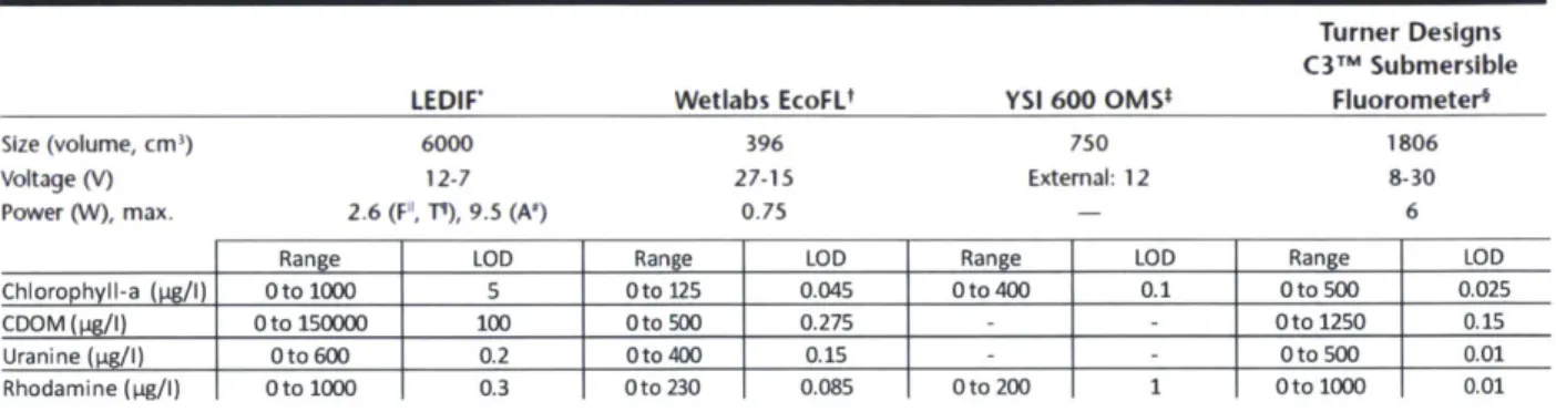
Commercial suppliers such as WET Labs, Turner Designs, Seapoints, and YSI produce optical sensors specifically designed for measurements in natural waters, including spectrometers for absorbance measurements, turbidity sensors, and fluorometers for measuring specific

compounds or chemical groups such as dissolved organic matter, crude oil, rhodamine, and chlorophyll. The sensors generally use a single LED excitation source and an emission detector with a filter, with LED and filter both chosen for the optimum wavelength bands for the

parameter of interest. The output of a single-wavelength-pair fluorometer, however, is

intrinsically incapable of identifying or correcting for interferences [18]. Ocean Optics Inc. and StellarNet Inc. both supply spectroscopy accessories such as spectrometers and fiber optics that are generally smaller, easier to use, and less expensive than typical laboratory equipment, and which have been applied to environmental analyses [15]-[17], [19], [20].

To the authors' knowledge, however, no low-cost instrument capable of deployment aboard a small AUV and exploiting both the spectral absorbance and the fluorescence EEM of natural waters yet exists. This paper provides details for a field instrument, named LEDIF, that has been built to address this need, and is made possible by advances in LED technology, advances in commercially available optical components, advances in low-cost single board microcomputers, and a valuable and a growing literature discussing LED-based field

instruments. LEDIF measures fluorescence, absorbance, and turbidity of natural waters. It is specifically designed for incorporation as a payload module of a STARFISH developed by National University of Singapore Acoustic Research Laboratory [21] or the MIT Sea Grant Reef Explorer, but with some variation in packaging can be used manually or can be installed on multiple other types of autonomous platforms. Applications include but are not limited to long-term monitoring, guiding rapid response to environmental chemical releases, developing adaptive sampling strategies for autonomous vehicles, and facilitating basic water quality research. This manuscript discusses the design and optical performance of LEDIF; equally important issues of signal processing will be discussed elsewhere.

2.2

Materials and Procedures

2.2.1 Sensor Module Overview

The layout of LEDIF and its typical modes of deployment are shown in 1.1.1. 1Figure 2.1. The optical functions of LEDIF rely on a custom designed flowcell fitted with light emitting diodes (LEDs) of different wavelengths, focused on the analytical volume and oriented 90 degrees from the main axis of light collection by a series of adjustable optics. To measure absorbance, a broadband (185 to 1100 nm) light source coupled via an optical fiber illuminates the flowcell at 180 degrees to the light collection system. Turbidity is also estimated within the flowcell by measuring the amount of excitation light scattered at 90 degrees (i.e. nephelometry).

For all measurements (fluorescence, absorbance, and turbidity), light from the flowcell is observed with an Ocean Optics USB4000 spectrometer, and the data are recorded with a single board computer running custom software under a Linux operating system. LEDIF uses switching

DC-DC converters to efficiently provide 5 and 12 VDC to various subsystems from either an

internal battery or from any external power supply voltage between 12 and 72 volts DC (VDC), a range which encompasses voltages used on a very large number of AUVs.

2.2.2 Flowcell geometry

A compact [-37(W) x 61(L) mm] optical flowcell permits the measurement of a water's

fluorescence spectrum, absorbance spectrum, and turbidity within the same analytical volume

(1.1.1. iFigure 2.2). The optic junctions for optical attachment use UV transmissive fused silica

windows with O-ring seals. Six junctions arranged perpendicular (90 degrees) to the detecting optic junction are used to provide excitation to the analytical volume for fluorescence and turbidity measurements. A similar optic junction arranged directly opposite (180 degrees) to the light-collecting optic junction is used to illuminate the volume for absorbance measurement. A collector lens, with focal length equal to the distance from the lens to the optical intersection with the perpendicular excitation optical paths, is fitted in front of the detecting optic junction to enhance collection of light emitted by fluorescence. Fluid flow into the flowcell occurs via a pathway that contains two 90 degree bends to minimize the entrance of stray light.

2.2.3 Excitation-Emission Optical System

A series of [-12.7(Dia) x 25.4(L) mm to 12.7(Dia) x 50.8(L) mm] LED-based light

sources produce optical excitation for the analytical volume. The light produced by the LEDs is focused to the geometrical center of the flowcell, in line with the detection optical path, using compound lenses chosen to accommodate the divergence angle associated with each respective

LED. The lenses are mounted inside lens tubes, and optical adjustments are performed using

retaining rings, which are locked in place after adjustment to minimize susceptibility to

mechanical disturbances. This compact packaging allows each excitation LED to be connected directly to the flowcell without the use of optical fiber, as shown in 1.1.1. 1Figure 2.2. For absorbance measurement, the light produced by a broadband (185 to 1100 nm) deuterium-tungsten (12 VDC at 0.6 A) source is focused with a plano-convex lens into an optical fiber, and

the exiting light is collimated with another plano-convex lens and redirected with a right angle prism mirror to the optic junction of the flowcell. A collector lens with a single core fiber is used for the collection of photons from fluorescence and scattering, and for collection of transmitted light in absorbance mode.

2.2.4 Power Control Board

The instrument requires a custom circuit board for power conditioning. 1.1.1. 1Figure 2.3 shows the block diagram of the power control board of LEDIF, which powers various loads at 5 or 12 VDC. It provides efficient DC-DC conversion of external power at 12 to 72 VDV (e.g. from a 48 V AUV battery) to 5 VDC and 12 VDC. One 5 VDC output for the embedded computer is always on when the board is powered. Two outputs of 5 VDC at 2.5 A maximum and one output of 12 VDC at 2.5 A maximum are provided; these are used (at less than their maximum current ratings) to power the spectrometer and the deuterium-tungsten light source. Eight current-limited outputs at user selectable 5 VDC or 12 VDC, rated up to 100 mA, are provided for the excitation LEDs. Three 5 VDC software-controlled variable-current outputs are supplied for future expansion, such as alternate broadband light sources for absorbance

measurement, or shorter-wavelength excitation sources that may become available in the future.

2.2.5 Computer

The sensor is controlled by an onboard single-board-computer (SBC) manufactured by Technologic Systems (Model TS-7260-64-128F). The TS-7260 uses an ARM9 200 Mhz CPU with 64 MB of RAM, 128 MB of Flash memory, and 2 GB (expandable) USB flash storage, and runs a Debian Linux operating system (OS). The SBC has 3 serial COM ports, 2 USB ports, 1 Ethernet port, 30 digital input/output (DIO) pins, and two analog to digital converter (ADC) pins. The DIO and ADC pins are software controlled. A battery-backed real time clock retains

synchronized sensor-host clock information for mission time-stamp. An on-board temperature sensor allows direct measurement of board temperature in the field. The microcomputer uses Ethernet for communication with a host platform such as the STARFISH. In addition, a serial port (RS-232) can be connected to the SBC for software development and diagnostic purposes. The USB 2.0 (12 Mbits/s max) port is used for connection with the 2 GB of flash storage and a

microcomputer is connected to the power control board using the added TS-XDIO (PN: OP-XDIO) port. Further technical data can be found at:

(http://www.embeddedarm.com/documentation/ts-7260-manual.pdf).

2.2.6 Software

Custom software (iLEDLIF; the extra "L" refers to the capability to control laser-excited instruments as well as LED-excited instruments) was written to control all sensor functionality. iLEDLIF was designed to be easily configurable and to handle asynchronous communication between multiple devices. The software is written in C++ using standard C/C++ libraries, and runs within Debian Linux on the embedded TS-7260 computer. iLEDLIF handles

communication with external devices (e.g. spectrometer) over serial, USB, Ethernet, or DIO connections as well as with virtual devices implemented entirely in software (e.g. a data analysis

device). On startup iLEDLIF reads an XML configuration file to load the device modules currently connected to the sensor, which allows for easy customization of the sensor hardware

(e.g. changing excitation LEDs). Once all device modules have been initialized, iLEDLIF passes commands from the operator or AUV to the specific devices. iLEDLIF also has a built-in

scripting language which enables users to generate text files of series of commands without needing to write or compile C++ code. These text files can be written or modified in the field, allowing the operator to automate scanning and spectra storing processes for a specific mission.

2.2.7 Spectrometer

Light transmitted through the sample volume or emitted by fluorescence from the sample volume is quantified by an Ocean Optics USB4000 spectrometer, which uses an uncooled

TCD1304AP CCD (charge-coupled device) as its detector and is equipped with: (1) UV4 Quartz windows, (2) variable longpass order-sorting filters to block 2nd and 3rd order light (part number

OFLV-4), (3) a cylindrical lens to increase light collection efficiency by the CCD (part number

L4), and (4) the widest available entrance slit (200x 1000 [tm) to provide maximum light throughput. This slit width corresponds to a wavelength resolution of -7.5 nm. Although the spectrometer is capable of higher resolution using narrower slit settings, this setting is acceptable given the characteristically broad fluorescence emission peaks of most analytes of interest, and the larger slit width allows for greater spectrometer throughput. The detector response is

wavelength dependent; the manufacturer-specified number of received photons per count of output are 130 and 60 at 400 nm and 600 nm, respectively. The optical bench uses a f/4

asymmetrical cross Czerny-Turner design with a SMA 905 inlet fitting, and has a 0.22 numerical aperture at the inlet that is matched to the connecting optical fiber. The integration time for each emission spectrum capture is software selectable from 3.8 ms to 10 s. Further technical

information on the spectrometer is available at:

(http://www.oceanoptics.com/technical/USB4000operatinginstructions.pdf).

2.2.8 Sample Flow

To minimize power consumption when deployed on an AUV, LEDIF samples water without use of a pump, using ram pressure to drive fluid through the flowcell as the AUV moves. To verify satisfactory flow conditions, three-dimensional transient flow modeling of the (x-z

plane) symmetrical liquid chamber (meshed with 212,016 cells of hybrid hex/tet mesh) was performed with Fluent (Version 12) software. The typical (0.21 million cells) mesh captured flow features identical to those obtained with a high density (1.05 million cells) mesh

(1.1.1. Figure 2.4(d) and (e)), showing the adequacy of the chosen mesh density. Flow through a LEDIF mounted aboard a STARFISH was simulated for several vehicle velocities, to visualize

the flow and determine if flow was obstructed, as well as to estimate the time required for water parcels both to reach the flowcell and to be flushed out. Each elbow was found to generate a local circulation that reduced the effective cross-sectional diameter of the flowpath. Particles were tracked to determine chemical transport and residence times; typical particle pathlines are shown in 1.1.1. iFigure 2.4(b). The model shows that all tracked particles (335 particles tracked for high density mesh and 91 particles tracked for typical mesh) escape through the outlet, with the maximum transit time for 95% of particles plotted in 1.1.1. 1Figure 2.4(c) at various vehicle velocity conditions. Transit time was approximately 0.8 s at the standard 3 knot cruising speed of STARFISH. This value is shorter than a typical measurement duration (several seconds), and therefore it is concluded that the sample flow does not limit data spatial resolution.

2.3Assessment

nm) as the source of excitation, and records emission spectra from 200 to 900 nm. The wavelengths in the PE LS-55 are selected with an excitation monochromator and an emission monochromator. The manufacturer's stated wavelength accuracy is +/-1 nm with a scanning speed of 10 to 1500 nm / minute with 1 nm increments. The signal-to-noise ratio is stated as

2500:1 RMS at the baseline and 750:1 RMS for observing water Raman using 350 nm as

excitation (http://www.perkinelmer.com/Catalog/Product/ID/L2250107).

2.3.1 Fluorescence Peak Validation

Fluorescence peaks are assessed by comparing the fluorescence spectrum of an aqueous solution of rhodamine B and chlorophyll a measured with LEDIF against the corresponding spectrum from the PE LS-55 (1.1.1.lFigure 2.5). For spectrum display purposes the emission spectrum intensity of the PE LS-55 is normalized by a factor equal to ILEDIF(Saturation) / JPE(Saturation)=

-63.5. This normalization is for display purposes only and is not an attempt to correct the spectra

for differences in wavelength specific response. The emission peaks of rhodamine B and chlorophyll a observed by the two sensors are in agreement within 1 nm; the emission peaks of rhodamine B and chlorophyll a reported by LEDIF were at 575 nm and 677 nm, respectively, agreeing well with values from the literature. For LEDIF, the peak amplitude of 405 nm is higher than 370 nm because the optical output of the 405 nm LED is approximately 4 times that of the

370 nm LED.

2.3.2 Field Samples Comparison

Emission spectra of pore waters collected from multiple depths at a peatland in Brunei are shown in 1.1.1.1 Figure 2.6. The fluorescence of these waters is attributed primarily due to high levels (10s of mg/L) of dissolved organic carbon (DOC). Emission spectra from LEDIF at 405 nm excitation and the PE LS-55 at 390 excitation were measured. The fluorescence peak

from LEDIF is shifted longer by -50 nm compared to the PE LS-55. This shift can be attributed to the longer excitation wavelength and the wavelength dependent response of the USB4000

which has not been corrected for with this data. Both LEDIF and the PE LS-55 instruments captured an -15% increase in fluorescence maxima as the depth from which the samples were collected increased.

2.3.3 Multi-spectral and EEM Demonstration

The ability of LEDIF to capture an emission-excitation matrix is demonstrated by measuring an aqueous solution containing five chemicals, each relevant to natural water studies. 1 ppm naphthalene, 135 ppb pyrene (i.e. at its solubility), 5 ppm of a commercial humic acid, 0.2 ppm rhodamine B, and 5 ppm chlorophyll a were selected to represent, respectively, a semi-volatile pollutant, a higher-molecular-weight semi-semi-volatile PAH, humic material, a widely-used tracer, and algal biomass. 1.1.1. 1Figure 2.7 shows the EEM of the mixture: each chemical peak can be clearly identified by inspection. Wavelengths of individual emission peaks of the

chemicals were compared with published fluorescence peaks from PhotochemCAD (Du et al.

1998) and found to be in very good agreement (1.].1. lFigure 2.7). Note that many of the data in

Du et al. (1998) are for compounds dissolved in a different solvent, potentially contributing to small differences in the location of fluorescence peaks.

Another meaningful comparison between LEDIF and the PE LS-55 is the instrumental detection limit (IDL). IDL is defined as:

IDL =

3a-where cy denotes standard deviation of repeated measurements at a single concentration. Using an excitation wavelength of 405 nm for both instruments, the detection limit of rhodamine B was

2.5 ppb and 2.1 ppb for LEDIF and the PE LS-55, respectively. For an excitation wavelength of 370 nm, the detection limit was 4 ppb and 3.2 ppb for LEDIF and the PE LS-55, respectively.

For the mixture described above, LEDIF had a detection limit of -50 ppb naphthalene, -7 ppb pyrene, -420 ppb humic acid, ~1 ppb rhodamine B, and -5 ppb chlorophyll a, with each detection limit being obtained at the optimum excitation wavelength.

2.3.4 Absorbance Measurement

The absorbance spectra at various concentrations of aqueous rhodamine B at its wavelength of maximum absorbance is shown in 1.1.1.lFigure 2.8(a). Based on 1.1.1.1Figure

2.8(b), absorbance as low as 0.01 was adequately measured by LEDIF at this wavelength. The

absorbance peak is observed at 552 nm, which falls within the range of 550-554 nm (shaded region) reported by the manufacturer (Panreac). In addition, the profile of the absorbance curve recorded by LEDIF was compared with the graph published by PhotochemCAD using ethanol as

curve and the pathlength (4.0 cm) of LEDIF's flowcell, the molar absorptivity was calculated as

0.17 L mol-1 cm-1 and the individual measurements at different concentrations are reported as 0.16 L mol-1 _{cm-1 (0.2 ppm), 0.19 L mol-}1 _{cm'(1 ppm), and 0.17 L mol-}1 _{cm' (2 ppm).} 2.3.5 Turbidity Measurement

Turbidity measurement was demonstrated using a calibration standard made of styrene divinyl benzene copolymer beads in water (AMCO CLEAR@TURBIDITY STANDARD

manufactured by GFS Chemicals, Inc). 1.1.1.1 Figure 2.9 shows the scattered light spectra using 405 nm excitation and various levels of turbidity, as well as resulting calibration curves for turbidity in the 0-1 Nephelometric Turbidity Unit (NTU) and 0-40 NTU ranges, using a 200 ms integration time. Three ranges of turbidity were tested: (1) 0 to 1 NTU in 0.2 NTU increments, (2) 0 to 10 NTU in 2 NTU increments, and (3) 0 to 40 NTU in 20 NTU increments. These ranges are representative of samples ranging from finished drinking water to many natural waters. 40

NTU does not reflect the upper bound limits of LEDIF, however, as higher turbidities can be

measured by using shorter integration times, different excitation wavelengths, or lower optical power. Turbidity as low as 0.1 NTU can be measured, demonstrating a potential application in monitoring processed drinking water, for which a typical upper limit specified by water authorities is 1 NTU.

2.3.6 Pressure and Temperature Effects

Given that LEDIF is intended for in situ deployment, the sensor response as a function of pressure was assessed using chlorophyll-a as an example from 0 to 120 psi gauge pressure. It was found that the effect of pressure on sensor response was less than 2% difference, which is immaterial. There is no evidence that LEDIF response to temperature at any anomalous function and we anticipate this affects LEDIF similar to other instruments. Fluorescence is known in general to decrease with increased temperature [22], although the dependence varies among compounds; Downing et al. [23] have measured the temperature dependence for the case of DOM. The STARFISH vehicle, and likely most other platforms on which LEDIF would be deployed, carries a temperature sensor that may be used for temperature corrections if desired. A second possible temperature effect occurs via mechanisms that cause instrument response to vary with temperature. The USB4000 spectrometer CCD has 13 black pixels that are not exposed to