HAL Id: insu-00604949
https://hal-insu.archives-ouvertes.fr/insu-00604949
Submitted on 30 Jun 2011HAL is a multi-disciplinary open access archive for the deposit and dissemination of sci-entific research documents, whether they are pub-lished or not. The documents may come from teaching and research institutions in France or abroad, or from public or private research centers.
L’archive ouverte pluridisciplinaire HAL, est destinée au dépôt et à la diffusion de documents scientifiques de niveau recherche, publiés ou non, émanant des établissements d’enseignement et de recherche français ou étrangers, des laboratoires publics ou privés.
Connectivity-consistent mapping method for 2-D
discrete fracture networks
Delphine Roubinet, Jean-Raynald de Dreuzy, Philippe Davy
To cite this version:
Delphine Roubinet, Jean-Raynald de Dreuzy, Philippe Davy. Connectivity-consistent mapping method for 2-D discrete fracture networks. Water Resources Research, American Geophysical Union, 2010, 46, pp.W07532. �10.1029/2009WR008302�. �insu-00604949�
1
Connectivity-consistent mapping method for 2D discrete fracture networks
1Delphine Roubinet, Jean-Raynald de Dreuzy and Philippe Davy 2
Geosciences Rennes, UMR CNRS 6118, Université de Rennes I, Rennes, France 3
Abstract
4
We present a new flow computation method in 2D Discrete Fracture Networks (DFN) intermediary 5
between the classical DFN flow simulation method and the projection onto continuous grids. The 6
method divides the simulation complexity by solving for flows successively at a local mesh scale and 7
at the global domain scale. At the mesh scale, flows are determined by classical DFN flow 8
simulations and approximated by an Equivalent Hydraulic Matrix (EHM) relating heads and flow 9
rates discretized on the mesh borders. Assembling the Equivalent Hydraulic Matrices provides for a 10
domain-scale discretization of the flow equation. The Equivalent Hydraulic Matrices transfer the 11
connectivity and flow structure complexities from the mesh scale to the domain scale. Compared to 12
existing geometrical mapping or equivalent tensor methods, the EHM method broadens the 13
simulation range of flow to all types of 2D fracture networks both below and above the 14
Representative Elementary Volume (REV). Additional computation linked to the derivation of the 15
mesh-scale Equivalent Hydraulic Matrices increases the accuracy and reliability of the method. 16
Compared to DFN methods, the EHM method first provides a simpler domain-scale alternative 17
permeability model. Second, it enhances the simulation capacities to larger fracture networks where 18
flow discretization on the DFN structure yields system sizes too large to be solved using the most 19
advanced multigrid and multifrontal methods. We show that the EHM method continuously moves 20
from the DFN method to the tensor representation as a function of the mesh-scale discretization. The 21
balance between accuracy and model simplification can be optimally controlled by adjusting the 22
domain-scale and mesh-scale discretizations. 23
2 24
1. Introduction
25
Fractured media has been classically modeled using either Discrete Fracture Network (DFN) or 26
Stochastic Continuum (SC) approaches [Neuman, 2005]. Both approaches have their own advantages 27
and drawbacks [Hsieh, 1998]. First, they differ by their underlying permeability structure and their 28
capacity of being specified by existing field data [Hsieh, 1998]. The DFN approach easily accounts 29
for extensive fracture characterization [Cvetkovic et al., 2004; Davy et al., 2006] while the SC 30
approach copes more consistently with hydraulic data [Ando et al., 2003]. Second, the simulation of 31
hydraulic processes requires the development of specific methods using the DFN approach whereas 32
only standard discretization schemes are required with the SC approach. Third, because the SC 33
approach simplifies the fracture network structure, it is generally less computationally demanding 34
than the DFN method. Hybrid approaches have been developed to combine the advantages of the 35
DFN and SC approaches. Most of them use a DFN approach at the onset for building equivalent 36
heterogeneous continuous models mapping either the smallest fractures [Lee et al., 2001] or all 37
fractures in the case of the Fracture Continuum Model (FCM) [Botros et al., 2008; Bourbiaux et al., 38
1998; Jackson et al., 2002; Reeves et al., 2008; Svensson, 2001]. Fracture Continuum Models aim at 39
benefiting both from the structure complexity of DFNs and from the simulation and computational 40
simplicities of continuous media. The objective is often to use the FCM approximation as a basis for 41
simulating more computationally demanding transient or multiphase flows [Bourbiaux et al., 1998; 42
Karimi-Fard et al., 2006]. 43
The quality of the FCM models critically depends on the derivation of the block-scale permeabilities 44
from the DFNs, i.e. on the mapping of the fracture network onto the continuum grid. The block is 45
considered here as the elementary cell of the continuum grid. Block-scale permeabilities are obtained 46
either from geometrical characteristics [Botros et al., 2008; Svensson, 2001] or through block-scale 47
3
numerical simulations of flow [Jackson et al., 2002]. Potential errors stem from differences between 48
the derived scalar or tensor permeabilities and the effective flows within the block. They arise from 49
the difficulty to account for complex fracture connectivity on a broad range of scales. For mapping 50
based on geometrical rules, errors decrease with finer discretization whereas for mapping based on 51
hydraulic computation of the equivalent permeability tensor, errors increase below the 52
Representative Elementary Volume [Long et al., 1982]. Jackson et al. [2002] corrected part of the 53
latter error by using a larger simulation zone, namely the “guard zone”, designed to remove dummy 54
additional fracture connectivity with the sides of the block. FCMs keep the general connectivity 55
structure above the scale of the block but remove most of the connectivity effects at lower scales. 56
This results in less flow localization at the block scale and in difficulties in defining an equivalent 57
block permeability tensor. A simple assessment criterion of the relevance of the tensor representation 58
is the difference between flows on opposite block faces. They are equal in the tensor representation. 59
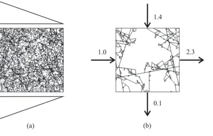
Their difference is expected to increase steeply for complex networks below the REV scale as shown 60
in the example of Figure 1. To avoid handling complex connectivity at the block scale, existing FCM 61
methods are applied either at scales close to the smallest fractures modeled [Botros et al., 2008; 62
Reeves et al., 2008] or at scales larger than the Representative Elementary Volume (REV) 63
[Durlofsky, 1991; Jackson et al., 2002]. The first methods, i.e. the methods applicable to scales close 64
to the smallest fracture modeled, represent permeability by a scalar or a diagonal tensor. They 65
require fine grids for fractured medium representation but can be highly accurate for not too dense 66
fracture networks [Botros et al., 2008]. The second methods, i.e. the methods applicable to scales 67
larger than the REV, represent permeability by an anisotropic full tensor defined by three 2D 68
parameters Kxx, Kyy and Kxy=Kyx. They require the a priori knowledge of the REV and are hence more
69
suited to dense fracture networks. Their drawbacks are the strong homogenization of flow, their 70
applicability to a restricted scale range and the increase of the numerical error with the refinement of 71
discretization. 72
4
None of these methods applies between the scale of the smallest fractures modeled and the REV, a 73
scale range that spans orders of magnitude for multiscale fracture networks (i.e. fracture networks for 74
which the fracture-length distribution is a power law) [Bonnet et al., 2001; de Dreuzy et al., 2001b]. 75
In fact, this scale range extends at least from the connectivity scale to the REV scale. The 76
connectivity scale is the scale at which networks are just connected. It ranges from meters to 77
kilometers [Berkowitz et al., 2000; Davy et al., 2009]. Because of the fracture transmissivity 78
variability, the REV scale can be one to three orders of magnitude larger than the connectivity scale 79
[Baghbanan and Jing, 2007; de Dreuzy et al., 2001a; 2002]. Extending at least from the scales 80
contributing to connectivity to the REV scale, the scale range of fractures contributing to flow covers 81
several orders of magnitude from the meter to the kilometer scale. For this scale range, the only 82
available flow simulation method is the DFN method. The DFN flow simulation method, however, is 83
limited in terms of fracture number and domain size. The limiting step arises when solving the linear 84
system issued from the flow discretization on the network structure. With traditional system-solving 85
methods like the conjugate gradient, limitations stemmed from computation time. However, the new 86
numerical methods like the multifrontal or algebraic multigrid method, as implemented in 87
UMFPACK [Davis, 2004] and HYPRE [Falgout et al., 2005], are orders of magnitude faster but 88
require additional memory [de Dreuzy and Erhel, 2002]. Their sole limitation is the computer 89
memory. As a rule of thumb, they can solve at most a linear system of rank one million in a couple 90
of minutes on a personal workstation (Pentium Xeon, 3 GHz, 8 Go). Consequently, improving 91
simulation capacities is not about speeding up the method but about enabling simulations otherwise 92
impossible because of memory requirements. We will thus look in this paper at the numerical 93
memory complexity rather than at the numerical time complexity. Our longer-term strategy is to use 94
parallel computing for performing Monte-Carlo simulations while sequential individual simulations 95
remain sequential [Erhel et al., 2009]. This ensures scalability and a minimum of parallel computing 96
implementation. 97
5
We propose a new FCM method for the scale range where no existing FCM method is applicable. 98
Like with the previously-cited FCM methods, the objective is to simplify the domain-scale numerical 99
scheme and computations while keeping the complexity of the DFN structure. The new method 100
divides the simulation complexity by solving for flows successively at the local block scale and at 101
the global domain scale. At the block scale, flows are determined by classical DFN flow simulations 102
and approximated by an Equivalent Hydraulic Matrix (EHM) relating heads and flow rates 103
discretized on the mesh borders. Assembling the Equivalent Hydraulic Matrices allows for a domain-104
scale discretization of the flow equation. The Equivalent Hydraulic Matrices transfer the connectivity 105
and flow structure complexities from the block scale to the domain scale. The method is similar to 106
Boundary Element Methods [Dershowitz and Fidelibus, 1999] as it relates heads and flow rates on 107
the block borders. As the Equivalent Hydraulic Matrices are determined at the block scale by DFN 108
simulations, we show that the method is systematically applicable regardless of the scale, fracture 109
density and fracture-length and transmissivity distributions. The method accuracy and complexity are 110
given by the level of discretization of the block borders and of the domain. We call this method the 111
Equivalent Hydraulic Matrices (EHM) method as heads and flow rates on the block borders are 112
linearly linked by a matrix representing the block-scale hydraulic properties rather than by a scalar or 113
a tensor permeability. This article describes the EHM method (section 2), shows its results compared 114
to existing methods (section 3) and discusses its performance (section 4). 115
2. The Equivalent Hydraulic Matrices method
116
This section defines the EHM method. Once the domain meshed into elementary blocks, the 117
principle of the EHM method is to express the block-scale hydraulic properties by a linear 118
relationship between discretized flow rates and heads on the block borders. This expression will 119
replace the scalar or tensor models used in classical FCM models. With 𝒑𝒌 as the discretization
120
points (also called poles) of the block numbered k, the vector of flow rates 𝝓𝒌 and heads 𝑯𝒌 on these 121
6 points are related by the following linear relationship: 122
𝝓𝒌 = 𝑨𝒌∙ 𝑯𝒌. (1)
123
The block matrix 𝑨𝒌 contains sub-block scale connectivity information and can be considered as the 124
block-scale constitutive relationship. It is obtained by performing block-scale flow simulations on 125
the DFN. Once obtained, the block-scale matrices 𝑨𝒌 are used for simulating flow rates at the system
126
scale by imposing the continuity of heads and flow rates across the block borders. Relationship (1) 127
differs a priori from Darcy’s law by its relating flow rates to heads and not to head gradients. This is 128
only a surface difference since the construction method (section 2.2) and the resulting properties of 129
matrices 𝑨𝒌 (Appendix A) ensure a dependence of the flow rates on head gradients. 130
2.1. Discretization
131
Discretization is made up of two parts consisting in discretization of the domain into elementary 132
blocks (classical meshes) and discretization of block borders into poles. The first discretization 133
consists in defining the mesh of the Fracture Continuum Model. We use hereafter a regular grid even 134
though the EHM method can cope with irregular meshes. Each mesh cell will be called a block. The 135
block contains a subset of the fracture network, i.e. a sub-network, the intersections of which with 136
the block limits are denoted 𝒎𝒌. 𝒎𝒌(𝑖) is the ith intersection of block k. The second discretization 137
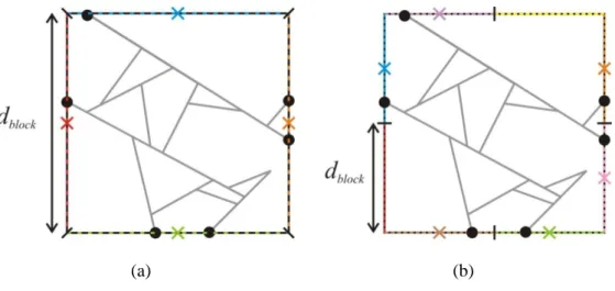
consists in splitting up the block borders into segments of constant length dblock, the discretization of
138
each border starting at the border corner. Each segment contains either zero, one or more than one 139
fracture border intersection 𝒎𝒌(𝑖). We define poles 𝒑𝒌 as the centers of those segments containing at 140
least one intersection (Figure 2). Segments containing no intersection with the subnetwork are 141
disregarded. The fundamental principle of the EHM method is that all intersections contained in the 142
same segment are set to the same hydraulic head corresponding to the head of the pole. These 143
additional equalities reduce the number of unknowns at the cost of the approximation that close 144
7
intersections have the same hydraulic head. The accuracy of the approximation is function of the 145
block discretization ratio rblock defined as the block-border discretization scale dblock normalized by
146
the block face length. The coarsest discretization corresponds to rblock=100% and gives a single pole
147
by block face. It leads to a representation close to the tensor representation (Figure 2a). It is, 148
however, not equal to a tensor. First, opposite fluxes may not be equal. Second, some faces may not 149
be intersected by the network and thus may not have led to a pole. Finer discretizations, obtained for 150
decreasing rblock values, lead to more accurate representations converging to the DFN method when
151
all poles correspond exactly to one intersetion (Figure 2b). Like in classical numerical methods, we 152
will show in section 3 that the numerical error of the EHM method decreases monotonously with the 153
block-border discretization ratio rblock, i.e. when shifting from tensor-like to DFN methods.
154
2.2. Construction of the block-scale Equivalent Hydraulic Matrices
155
Equivalent Hydraulic Matrix 𝑨𝒌 expresses the linear relationship between flows and heads on the
156
block border discretization. More specifically, by developing relationship (1), coefficient 𝑨𝒌(𝑖, 𝑗) is 157
the contribution of the head at the jth pole to the flow at the ith pole: 158
𝝓𝒌(𝑖) = 𝑁𝑃 𝑨𝒌 𝑖, 𝑗 ∙ 𝑯𝒌(𝑗)
𝑘
𝑗 =1 . (2
159
where 𝑁𝑃𝑘 is the pole number of block k and 𝝓𝒌(𝑖) and 𝑯𝒌(𝑖) are the flow rate and head, 160
respectively, at ith pole 𝒑𝒌(𝑖). 𝑨𝒌(𝑖, 𝑗) is also equal to the flow rate computed at pole i by imposing a 161
fixed head of 1 at pole j and 0 at the other ones, i.e. a fixed head of 1 for the intersections overlapped 162
by the segment centered on pole j and 0 for the other ones. With these boundary conditions, all 163
coefficients of column j can be simultaneously determined by a single DFN simulation (Figure 3). 164
The construction of the full Equivalent Hydraulic Matrix requires 𝑁𝑃𝑘 − 1 simulations and not 𝑁𝑃𝑘, 165
since the sum of all elements from a column of 𝑨𝒌 is equal to zero because of flow conservation
8
(Appendix A). We underline that this method does not require any modification of the fracture 167
network structure or any realignment of fractures. The approximation lies exclusively in equating 168
flows and heads at the scale of the segment of the border discretization. 169
2.3. Domain-scale flow simulation
170
Solving the flow equation at the domain scale consists in imposing the continuity of heads and flow 171
rates on poles 𝒑𝒌 positioned on the block faces. External head and flow rate boundary conditions are
172
simply implemented by imposing the head in the matrix system for the fixed head values and by 173
adding a source term for the fixed flow rates on the corresponding poles, respectively. 174
We note P the union of all pole points 𝒑𝒌 with the convention that poles common to two or more 175
blocks occur only once in P. P is made up of Ni poles at the interface between two blocks (P i) and of 176
Nf poles at the physical limits of the domain (P f). The total number of poles at the domain scale N is 177
equal to the sum of poles of types 𝑃𝑖 and 𝑃𝑓:
178
𝑁 = 𝑁𝑖 + 𝑁𝑓. (3)
179
With B(j) as the set of blocks sharing pole 𝑃𝑖(𝑗) and with 𝑞
𝑏,𝑃𝑖(𝑗 ) as the flow rate at pole 𝑃𝑖(𝑗) from
180
the bth block of B(j), flow continuity writes: 181
𝑞𝑏,𝑃𝑖(𝑗 )
𝑏 𝜖 𝐵(𝑗 ) = 0 ∀𝑗𝜖 1, 𝑁𝑖 . (4)
182
For the Nfd fixed poles at the domain limit where a Dirichlet boundary condition is applied: 183
𝐻𝑓𝑑 = 𝐻𝑓𝑑
0. (5)
184
For the Nfn poles on the Neumann boundary condition, the imposed flow is simply inserted in 185
9
equation (4). Equations (1), (4) and (5) lead to a linear system of N equations of the N unknown 186
heads at the poles. 187
The first advantage of the EHM method compared to existing Fracture Continuum Models (FCMs) 188
is the conservation of connectivity between blocks. In fact, faces intersected by fractures contain at 189
least one pole whereas faces without intersecting fractures do not have any pole. This prevents 190
dummy additional connectivity between blocks [Jackson et al., 2002; Reeves et al., 2008]. The 191
second advantage of the EHM method is the existence of block-scale discretization parameter rblock,
192
which can be used to tune the balance between numerical efficiency and accuracy. The third 193
advantage of the method is the systematic convergence with discretization and its adjustment to all 194
kinds of 2D synthetic fracture networks as will be shown in section 3. The main drawbacks of the 195
EHM method are the necessity to perform block-scale DFN flow simulations and the specificity of 196
the domain-scale flow simulation that precludes the use of standard softwares like MODFLOW. 197
3. Results
198
3.1. Fracture network types
199
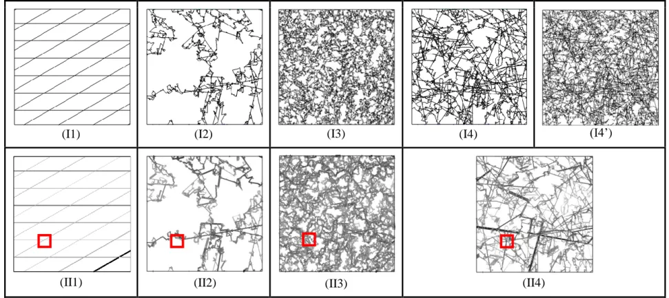
The tested networks have been chosen so that they cover a wide range of networks both above and 200
below the REV scale, with broad and narrow length and transmissivity distributions (Table 1). 201
Extreme cases of low and high variability are tested in order to assess the method in highly-202
differentiated conditions. Network types include both lattice structures (Table 2.I1) and stochastic 203
complex fracture networks (Table 2.I2-4). Stochastic fracture networks are characterized by their 204
density, orientation, length and transmissivity distributions. The domain size given by the ratio of the 205
domain length to the minimal fracture length is denoted by L and set to 100. It means that the 206
fracture length distribution covers two orders of magnitude. Density is fixed by the dimensionless 207
percolation parameter p, equal to the sum of the square of the fracture lengths normalized by the 208
10
domain area. p is a direct measure of connectivity as it is very close to 5.6 at the percolation 209
threshold, whatever the other fracture network characteristics [Bour and Davy, 1997]. Three density 210
values are used for stochastic complex fracture networks and are respectively close to threshold 211
(p=6) and at around two and three times the density at threshold (p=10 and p=20). For lattice 212
structures, p is close to the number of fractures within the domain and has been chosen equal to 12 213
and 192 for testing methods on sparse and dense lattices, respectively. Orientations are set to 0° and 214
30° relative to the main flow directions for the lattice structures and are uniformly distributed for the 215
complex stochastic fracture networks. For the complex stochastic fracture networks, fracture lengths 216
are power-law distributed [Bonnet et al., 2001] according to the following distribution function: 217
𝑝 𝑙 ~𝑙−𝑎 (6)
218
where l is the fracture length, a is the characteristic power-law length exponent and 𝑝 𝑙 the fracture 219
number of length l. Natural values of a derived from outcrops range in the interval [2.0,3.5]. Fracture 220
transmissivity values have been chosen to be either the same for all fractures or broadly distributed 221
according to a lognormal distribution of logarithmic standard deviation equal to 3 [Tsang et al., 222
1996]. Flow boundary conditions are classical gradient-like boundary conditions with fixed head on 223
two opposite domain faces and a constant head gradient on the orthogonal faces (Figure 1a). The 224
bottom line of Table 2 illustrates the flow distribution computed with a broad transmissivity 225
distribution and shows the strong channeling induced by the transmissivity distribution. 226
3.2. Comparison criteria
227
For comparing the performance of the EHM method with other existing methods, we use an accuracy 228
criterion and a numerical memory complexity criterion. Accuracy is defined as the mean difference 229
between the inlet and outlet flows and their reference counterparts. The reference is obtained from 230
11
the direct simulation on the domain-scale discrete fracture network. By denoting Φ𝑚𝑓𝑖 and Φ𝑟𝑒𝑓𝑓𝑖 the 231
flow rates obtained respectively by the method “m” and the reference method on face 𝑓𝑖, the
232
comparison criterion writes: 233 𝑓𝑙𝑜𝑤_𝑒𝑟𝑟𝑜𝑟𝑚 =12 Φ𝑚𝑓𝑙−Φ𝑟𝑒𝑓𝑓𝑙 Φ𝑟𝑒𝑓𝑓𝑙 + Φ𝑚𝑓𝑟−Φ𝑟𝑒𝑓𝑓𝑟 Φ𝑟𝑒𝑓𝑓𝑟 × 100 (7) 234
where 𝑓𝑙 and 𝑓𝑟 stand for the left and right vertical domain faces. 235
The memory complexity criterion is taken as the number of non-zero elements nnz of matrix B in the 236
linear system Bx=b issued from the discretization of the flow equation at the domain scale. Even if 237
the number of non-zero elements is not the ideal criterion, it is still better than the system size in this 238
case where the limitation lies rather in memory requirements than in computation time. All results 239
represent averages over 10 simulations. We have checked that for the most complex cases D0 and 240
D1, 10 and 100 simulations give very close results. Accuracy and numerical memory complexity 241
results are computed for several discretizations characterized by the number of blocks (domain-scale 242
discretization) and by rblock (block-scale discretization).
243
3.3. Results with existing mapping and tensor methods
244
To assess the Equivalent Hydraulic Matrices method, we compare it with other existing methods: 245
first with what we call the ANIS_GEO method representing permeability by a diagonal tensor 246
derived from fracture geometrical mapping onto the blocks and used within a finite volume method 247
[Botros et al., 2008] and second with what we call the TENSOR_SIM method representing 248
permeability by a full tensor obtained from block-scale DFN flow simulations and used within a 249
mixed hybrid finite element framework (Appendix B). For these two methods, the matrix 250
permeability is fixed to 10-12 m/s. We use these two methods only when they are strictly applicable. 251
12
From [Botros et al., 2008], the ANIS_GEO method is applicable only if the ratio of the block length 252
to the minimal fracture length is lower than 2.5. For the stochastic complex networks (Table 1 B0-253
D1), the ratio of the domain size to the minimal fracture length is L=100, requiring for the 254
ANIS_GEO method a domain-scale discretization of at least 40×40 blocks. As the TENSOR_SIM 255
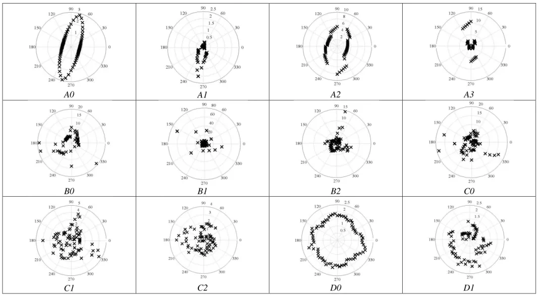
method relies on the full permeability tensor at the block scale, we have determined this parameter 256
for all studied networks from the block-scale directional permeability plots (Table 3). The method is 257
applicable only when the directional permeability is close to an ellipse [Long et al., 1982]. It is the 258
case for networks A0, A2 and D0 (Table 3). For the other networks, transmissivity and fracture 259
length distributions display heterogeneities that cannot be represented by a tensor at the scale of the 260
block. 261
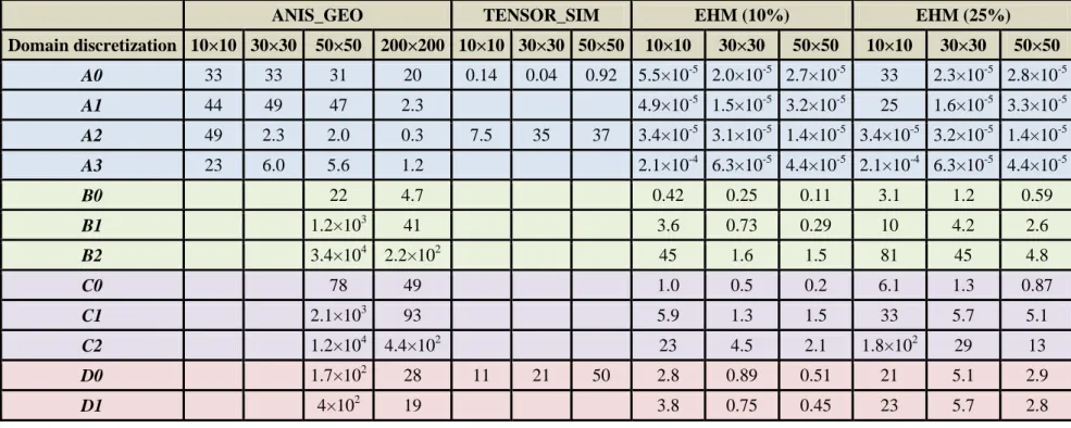
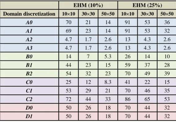
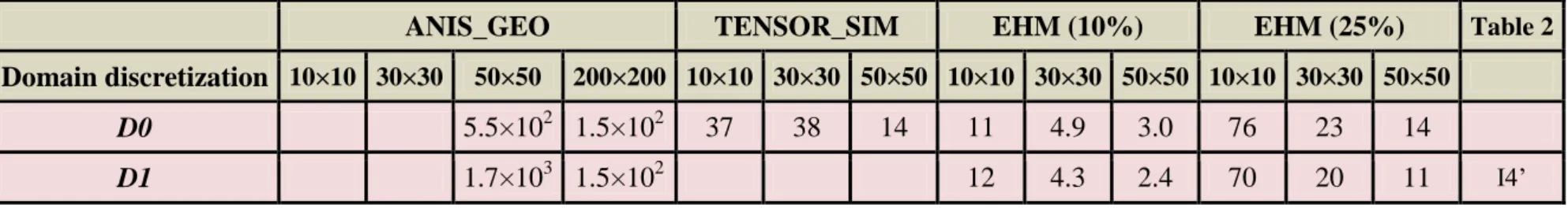
Table 4 shows the flow error as measured by (7) using the ANIS_GEO, TENSOR_SIM and EHM 262
methods for several domain discretizations. With the ANIS_GEO method, the flow error decreases 263
systematically from a 50×50 to a 200×200 domain discretization. ANIS_GEO is particularly accurate 264
for sparse flow structures (networks with a small fracture density or with a broad transmissivity 265
distribution). In fact, the simple summation of the fracture contributions induced by the mapping 266
increases sub-block-scale connectivity and hence increases flow errors. Results also show that 267
ANIS_GEO is not applicable to networks with connectivity driven by small fractures (3<a<3.5), 268
yielding errors systematically larger than 41%. To be applied systematically, the geometrical 269
projection method ANIS_GEO requires high levels of discretization involving large linear systems 270
(Table 5). Such discretization levels can be achieved in 2D but likely not in 3D. 271
The TENSOR_SIM method is accurate for regular and dense structures with an error lower than 1% 272
for network A0 (Table 4). As opposed to the ANIS_GEO method, the error decreases when the block 273
scale increases since the block becomes closer and eventually larger than the REV [Li et al., 2009]. 274
The main drawback of this method is its highly limited range of application. Most of the tested 275
13
networks of Table 1 did not fulfill its conditions of application. 276
3.4. Assessment of the EHM method
277
We have tested two levels of block-scale discretization of the EHM method: rblock=10% (called the
278
most accurate method) and rblock=25% (called the least accurate method). The EHM method gives
279
much smaller errors than those given by the geometrical and tensor methods ANIS_GEO and 280
TENSOR_SIM (Table 4) except for A0 (dense lattice structure with uniform fracture transmissivity) 281
and D0 (dense fracture network with uniform fracture transmissivity) with a domain discretized by 282
10×10 blocks and rblock=25%. For these two cases, the tensor method gives smaller errors than the
283
least accurate EHM method. In fact, the tensor method is very accurate because the REV is smaller 284
than the block. The large errors of the least accurate EHM method are linked to the large number of 285
fracture intersection points with the block border set to the same head, i.e. the head of the 286
corresponding pole. The merged points are quantified by the border merging percentage pborder equal
287
to the difference in percentage between the intersection point and pole numbers. pborder is 0% in the
288
absence of any approximation of the block-scale discretization and increases as larger 289
approximations are induced by the use of a smaller number of poles for the block-scale 290
discretization. For A0 and D0 with the 10×10 domain discretization and rblock=25%, pborder is larger
291
than 90% and 70%, respectively (Table 6). This explains the cases where the EHM method is less 292
accurate than the TENSOR_SIM method. For the same networks with finer domain discretizations 293
(30×30 and 50×50 blocks), trends are reversed and the EHM method becomes more accurate than 294
the tensor method. For lattice cases, the flow error with the EHM method is smaller than 5% for a 295
domain discretization of 50×50 blocks. 296
For stochastic complex fracture networks, flow errors range from 0.11% to 180% with a majority of 297
errors below 10% (Table 4). Errors larger than 10% affect cases B2 and C2 characterized by a coarse 298
14
discretization of 10×10 blocks and by networks with the narrowest length distribution corresponding 299
to a=3.5. The latter fracture networks have the largest number of fractures and fracture border 300
intersections inducing first a stronger decrease in the numerical memory complexity (Table 5), and 301
then larger values of point merging percentages pborder (Table 6). In all other cases, the flow error is
302
smaller than 5% for a domain discretization of 50×50 blocks. With the most accurate method 303
corresponding to rblock=10% and a domain discretization of 50×50 blocks, errors range between
304
0.11% and 2.1%. For 9 out of the 12 test cases for which 𝜎𝑙𝑛𝑇 = 3 corresponds to a fracture 305
transmissivity distribution spanning at least 3 orders of magnitude, errors remain as low as a few 306
percents showing the very good performance of the EHM method for complex flow structures. 307
Results of Table 4 show two interesting properties of the EHM method. First, errors are not sensitive 308
to the fracture transmissivity distribution as shown by the comparison of the D0 and D1 cases. 309
Second, errors systematically decrease both with the domain discretization at constant rblock and with
310
rblock at constant domain discretization for all complex stochastic fracture networks. These properties
311
offer possibilities to control the error by decreasing either the domain-scale discretization in blocks 312
or the block-scale discretization ratio rblock. We note that all the above simulations have been
313
performed on the backbone. However the applicability of the EHM method is not restricted to the 314
backbone as shown by its good performance on infinite clusters (Table 7). Even if errors increase by 315
a factor of 5 from the backbone to the infinite cluster, they still remain lower than 10% with the least 316
accurate method (rblock=10%) and a domain discretization of 50×50.
317
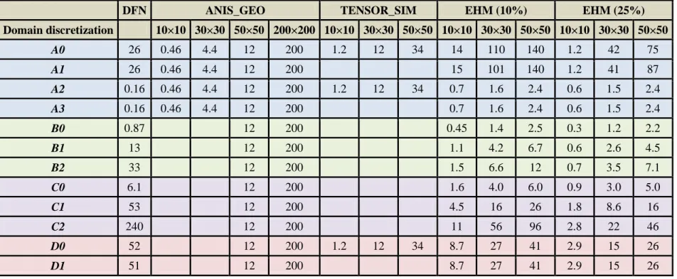
3.5. Flow error versus numerical memory complexity
318
Numerical memory complexity is taken as the number of non-zero elements in the domain-scale 319
linear system issued from the discretization of the flow equation (nnz) (Table 5). nnz determines the 320
memory required to solve the linear system. It does not, however, take into account the computation 321
15
of the Equivalent Hydraulic Matrices at the block scale as they are not critical in terms of system size 322
and memory requirements. With the classical ANIS_GEO and TENSOR_SIM methods, the 323
numerical memory complexity increases quadratically with the discretization ratio. With the EHM 324
method, the numerical memory complexity is more variable and increases more slowly. Whatever 325
the domain discretization and the value of rblock for complex stochastic fracture networks, EHM
326
methods yield smaller numerical memory complexity than the DFN method except for the B0 case. 327
In the latter case, the proportion of blocks crossed by a single fracture increases the numerical 328
memory complexity without improving the accuracy. 329
A more advanced evaluation of the methods is proposed by comparing their error according to their 330
numerical memory complexity (Figures 4-6). For lattice structures (Figure 4 except magenta 331
symbols), the EHM method is orders of magnitude more accurate than the classical methods at 332
comparable complexities except for the A0 case already discussed in section 3.4. Figure 4 also shows 333
that the accuracy of the TENSOR_SIM method increases with the numerical memory complexity as 334
discussed in section 3.3. For the dense complex stochastic fracture network of case D0 (Figure 4, 335
magenta symbols), the error with the TENSOR_SIM method is smaller than the error with all other 336
methods at very low complexity (11%) but cannot be made smaller by refining the discretization. By 337
contrast, with the EHM method, the error is larger at small complexity but decreases to less than 1% 338
for the highest complexities. For the stochastic complex fracture networks (Figures 5-6), errors with 339
the EHM method decrease with the numerical memory complexity (nnz), with a systematic trend 340
close to nnz-1. Figures 4-6 show that the errors using the EHM method with rblock=10% and rblock
341
=25% are roughly parallel in log-log plots. For the same level of error corresponding to horizontal 342
lines in Figures 4-6, the rblock =10% method yields smaller numerical memory complexities than the
343
method with rblock =25%.
344
3.6. Parameter optimization
16
The choice of the optimal method parameters depends on the targeted accuracy, available 346
computation time and memory and on the fracture network structure. We illustrate the methodology 347
to determine the appropriate parameter values on the most complex fracture network presented 348
before D1. Basically, we show in this section that the accuracy is controlled by the discretization 349
ratio rblock times the length of the block edge while computation time and memory requirements are
350
controlled by the inverse of the discretization ratio (1/rblock). The approximation of the method is
351
performed on the block-border discretization by equating the head of points belonging to the same 352
discretization segment. The sole parameter influencing accuracy is thus the normalized segment 353
length dblock equal to the discretization ratio rblock times the length of the block edge divided by the
354
minimal fracture length. The error error_flow defined in (7) increases monotonously with dblock
355
(Figure 7). Flow errors smaller than 20% are obtained for dblock values smaller than 2. Once the
356
segment length has been fixed by the targeted accuracy, the computation time and memory 357
requirements are adjusted by choosing the discretization of the system in blocks controlled by the 358
parameter 1/rblock (Figure 8). Here the computation time refers to the full time of the flow simulation
359
including the determination of the Equivalent Hydraulic Matrices and the solution of the large 360
system issued by the domain-scale flow discretization. Memory requirements are still taken as the 361
number of non-zero elements in the domain-scale matrix (nnz). As previously said, nnz decreases for 362
coarser domain discretizations. The computation is mainly controlled by the determination of the 363
Equivalent Hydraulic Matrices. It first sharply decreases with 1/rblock and then increases slightly. The
364
minimum expresses an optimal distribution of computations between the domain scale and the block 365
scale. Smaller 1/rblock values yield more numerous smaller blocks and more Equivalent Hydraulic
366
Matrices to determine and in turn an increase of the full computation time by more than order of 367
magnitude. Large 1/rblock values yield less numerous larger blocks which Equivalent Hydraulic
368
Matrices take a much larger time to determine, increasing the full computation time by at least 50%. 369
17
Similar results showing the existence of the minimum have been obtained for greater number of 370
Monte-Carlo simulations and for different fracture network structures. 371
4. Discussion
372
The principle of the Equivalent Hydraulic Matrices method is to distribute the numerical complexity 373
among two scales, the block-scale and the domain-scale. This method introduces a reduction of the 374
domain-scale numerical memory complexity by coarsening the block-border discretization. The 375
approximation consists in equating heads on nearby network points. It remains local and adjusts 376
automatically to the specific network configuration. Like the tensor and geometrical mapping 377
methods, the EHM method increases connectivity along block interfaces but only through the 378
introduction of shortcuts between existing paths and not through the connection of otherwise 379
disconnected faces. Moreover, the connectivity increase is limited to the block borders and does not 380
affect the connectivity within the block. 381
The EHM method is structured around the block-scale Equivalent Hydraulic Matrices, which transfer 382
the local connectivity information from the block scale to the domain scale. The Equivalent 383
Hydraulic Matrices are determined by the configurations of the fracture network within the blocks 384
but do not depend on the boundary conditions. In other words, the matrices are not intrinsic medium 385
properties like a tensor but can be used instead of the discrete fracture network in all flow contexts 386
both above and below the Representative Elementary Volume (REV). The Equivalent Hydraulic 387
Matrices method is still applicable below the REV due to the adjustment of the block-scale matrices 388
to the specificity of the connectivity structures. 389
Because the Equivalent Hydraulic Matrices are derived from DFN computations, it is not surprising 390
that they contain more information than the geometrical projection methods and lead to better 391
performance at equivalent scale numerical memory complexity. We express the domain-392
18
scale numerical memory complexity by the number of non-zero elements (nnz) of the linear system 393
issued from the discretization of the flow equation. nnz is two to four orders magnitude smaller with 394
the EHM method than with geometrical projection methods. The EHM method also displays 395
systematically decreasing flow errors with the domain discretization and block-scale discretization 396
parameter rblock. This offers possibilities to find the best optimal complexity for a given error
397
requirement. As seen in section 3.3, this is not possible with the tensor method TENSOR_SIM and it 398
requires too fine a domain discretization with the geometrical method ANIS_GEO. 399
The EHM method is intermediary between the full DFN flow simulation and the tensor method. Like 400
in the classical tensor methods [Jackson et al., 2002], the method relies on block-scale DFN 401
simulations. It is also similar to classical numerical methods from several respects. First, it expresses 402
the relationship between flows and heads on the block borders like many numerical methods such as 403
finite element or boundary element methods. Second, it converges to the full DFN solution when the 404
domain discretization or the block-scale discretization increases. As a two-scale method, it shares 405
similarities with multiscale methods like multigrid methods. It is, however, a pure bottom-up 406
approach in the sense that the block-scale information is used at domain scale but not the other way 407
around. From this respect, it is closer to the principle of the multiscale finite element methods 408
[Efendiev and Hou, 2007] than to the principle of multigrid methods [Wesseling, 2004]. Finally, it 409
remains opposed to homogenization methods since the Equivalent Hydraulic Matrices strongly 410
depend on the block-scale fracture network structure and cannot be extrapolated to other blocks or 411
other scales. 412
However, EHM methods have two drawbacks, the first one being the specificity of the domain-scale 413
simulation method that precludes the use of commonly available continuous flow simulation 414
softwares like MODFLOW. The second drawback is the additional numerical time complexity 415
arising from the computation of the block-scale equivalent matrices. The total numerical complexity 416
19
includes the solution of the domain-scale linear system and the computation of the Equivalent 417
Hydraulic Matrices at the block scale. The first contribution is evaluated by the number of non-zero 418
elements in the domain-scale linear system nnz used in the previous section. The second contribution 419
is a function of the number of scale simulations multiplied by the complexity of the block-420
scale simulations. We have chosen to retain only the first contribution to the numerical complexity 421
for the two following reasons. First, the complexity of the domain-scale linear system is a critical 422
constraint. Very large systems corresponding to nnz>107 require parallel computation. While this 423
constraint is met only for very large systems in 2D, it is current for 3D fracture networks at much 424
smaller domain scales. Second, the EHM methods will likely be interesting for transient simulations. 425
In fact, the computation of the EHMs will be performed only once and the complexity of the 426
transient simulations will depend only on the domain-scale linear system complexity. The choice of 427
both the domain discretization and the block-scale discretization parameter will be dictated by the 428
numerical optimization, the performance of simulations through block-scale and domain-scale 429
computations restricted to manageable sizes, and last but not least by the required accuracy. 430
5. Conclusion
431
We have presented a new mapping method for solving the flow equation in 2D discrete fracture 432
networks. The method consists in superposing a mesh onto the fracture network and finding the 433
relationship between heads and flows on the borders of each block of the mesh. The relationship is 434
linear and can be expressed in matrix form, hence the name the “Equivalent Hydraulic Matrices” 435
(EHM) method. We have shown that this linear relationship is fundamentally analog to Darcy’s law 436
as it is equivalent to relating flows to well-chosen head gradients on block borders. The matrix 437
coefficients can be determined by scale numerical simulations and express equivalent block-438
scale permeability between block border zones. The zones are chosen independently for each block 439
interface and correspond to the discretization of intersection points between the fracture network and 440
20
the block border. The method is parameterized both by the block-scale discretization parameter 441
(block-scale discretization distance divided by the characteristic block scale) and the domain 442
discretization (the domain scale divided by characteristic block scale in each direction). The flow 443
simulation at the domain scale is performed simply by assembling the block-scale Equivalent 444
Hydraulic Matrices through head and flow continuity conditions. 445
The interest of the EHM method is to keep good approximations of both the internal block and inter-446
block connectivities. Discretization is performed at a local scale and adjusts automatically to local 447
fracture network configurations. We show on a broad range of 2D fracture networks with different 448
density, fracture length and transmissivity distributions that the relative error of the method decreases 449
systematically with the domain discretization and the block-scale discretization parameter, allowing 450
for a possible automatic control of the method accuracy. We also show that the relative error of the 451
EHM method remains restricted to a few percents for a coarse domain discretization (30×30 to 452
50×50), whatever the network geometrical structure and the fracture transmissivity distribution. The 453
main advantage is its applicability to all kind of network structures, whereas the tensor method can 454
only be used for blocks larger than the Representative Elementary Volume, a too restrictive 455
condition for general DFN simulations. Geometrical methods give results of comparable accuracy 456
for a much larger domain discretization leading to domain-scale numerical memory complexities 457
orders of magnitude larger than the numerical memory complexity of the EHM method. The EHM 458
method enables large-scale 2D flow simulation networks. We intend to test its performance on 3D 459
fracture network simulations and in transient flow contexts. 460
21
Appendices
461
Appendix A: Property of the Equivalent Hydraulic Matrix
462
With the construction method described in section 2.2, 𝑨𝒌 has several properties. First, by imposing 463
a fixed head of 1 at pole j and 0 at the other ones as boundary conditions, the flow goes into the 464
block by 𝒑𝒌(𝑗) and outward through the other poles 𝒑𝒌(𝑖) (𝑖 ≠ 𝑗). Considering the flow going into 465
the block as positive and the flow going outward as negative leads to: 466
𝑨𝒌 𝑗, 𝑗 ≥ 0
𝑨𝒌 𝑖, 𝑗 ≤ 0, 𝑖 ≠ 𝑗 . (8)
467
Second, for a given column j, all elements 𝑨𝒌(𝑖, 𝑗) are determined simultaneously by solving the
468
flow equation; mass conservation implies that 469 𝑨𝒌 𝑖, 𝑗 𝑁𝑃𝑘 𝑖=1 = 0. (9) 470 Or similarly: 471 𝑨𝒌 𝑖, 𝑖 = − 𝑁𝑃 𝑨𝒌 𝑗, 𝑖 𝑘 𝑗 =1,𝑗 ≠𝑖 . (10) 472
Third, because the reciprocity principle is applicable in the case of Darcian flow [Barker, 1991], 𝑨𝒌 473
is symmetric: 474
𝑨𝒌 𝑖, 𝑗 = 𝑨𝒌 𝑗, 𝑖 . (11)
475
Fourth, we show that the linear relationship (1) between flows and heads with property (10) leads to 476
a relationship between flows and head gradients. In fact: 477
22 𝝓𝒌 𝑖 = 𝑨𝒌 𝑖, 𝑗 × 𝑯𝒌 𝑗 𝑁𝑃𝑘 𝑗 =1 𝝓𝒌 𝑖 = 𝑨𝒌 𝑖, 𝑗 × 𝑯𝒌 𝑗 + 𝑨𝒌 𝑖, 𝑖 × 𝑯𝒌 𝑖 𝑁𝑃𝑘 𝑗 =1,𝑗 ≠𝑖 and using (10): 478 𝝓𝒌 𝑖 = 𝑨𝒌 𝑖, 𝑗 × (𝑯𝒌 𝑗 − 𝑯𝒌(𝑖)) 𝑁𝑃𝑘 𝑗 =1,𝑗 ≠𝑖 𝝓𝒌 𝑖 = 𝑨𝒌 𝑖, 𝑗 × 𝑥𝑘,𝑖𝑗 ×(𝑯𝒌 𝑗 −𝑯𝑥 𝒌(𝑖)) 𝑘,𝑖𝑗 𝑁𝑃𝑘 𝑗 =1 (12) 479
where 𝑥𝑘,𝑖𝑗 is the distance between poles 𝒑𝒌(𝑖) and 𝒑𝒌(𝑗). Equation (12) shows that flow 𝝓𝒌 𝑖 at
480
𝒑𝒌(𝑖) is the sum of the head gradients from 𝒑𝒌(𝑖) to the other poles. Equation (12) gives a simple 481
interpretation of 𝑨𝒌 𝑖, 𝑗 × 𝑥𝑘,𝑖𝑗. 𝑨𝒌 𝑖, 𝑗 × 𝑥𝑘,𝑖𝑗 is the proportionality coefficient between flow 482
𝝓𝒌 𝑖 and the head gradient (𝑯𝒌 𝑗 − 𝑯𝒌(𝑖))/𝑥𝑘,𝑖𝑗 between 𝒑𝒌(𝑖) and 𝒑𝒌(𝑗). 𝑨𝒌 𝑖, 𝑗 × 𝑥𝑘,𝑖𝑗 can
483
thus be interpreted as an “equivalent transmissivity” between the ith
and jth poles. 484
23
Appendix B: Tensor permeability and finite elements (TENSOR_SIM method)
486
The Equivalent Hydraulic Matrices method consists in dividing the domain into blocks and 487
describing block-scale hydraulic properties using Equivalent Hydraulic Matrices. The discretization 488
of the block borders by poles 𝒑𝒌 is determined by the block-scale discretization parameter rblock,
489
which is the ratio of the block-scale distance discretization to the block length. This parameter rblock
490
drives the discretization of intersections 𝒎𝒌 between block borders and fractures. Coefficients of the 491
EHMs are determined by simulations at the block scale as described in section 2.2. The EHMs are 492
equivalent to tensors in that they impose the following discretization and construction rules: (1) 493
rblock=100%, i.e. each block border is discretized by at most one pole, (2) each block border is
494
represented by one pole (even if there is no intersection point), (3) matrix coefficients are determined 495
by applying head gradient boundary conditions in the vertical and horizontal directions [Renard et 496
al., 2001], (4) the computed flow rates used for the determination of the coefficients are the 497
directional flow rates, i.e. the mean of the flow rates going out of the domain through borders 498
perpendicular to the studied direction, and (5) coefficients are corrected to obtain symmetric positive 499
definite tensors [Long et al., 1982]. Adding these rules of determination, the Equivalent Hydraulic 500
Matrices become tensors that describe block-scale permeability. Computed block-scale tensors are 501
used within a classical mixed hybrid method adapted for quadrangles to simulate flow at the domain 502
scale [Chavent and Roberts, 1991]. We denote this method the TENSOR_SIM method. 503
24
Notations
505
Kxx permeability in the x-direction due to a head gradient in the x-direction, m/s.
506
Kyy permeability in the y-direction due to a head gradient in the y-direction, m/s.
507
Kxy permeability in the x-direction due to a head gradient in the y-direction, m/s.
508
Kyx permeability in the y-direction due to a head gradient in the x-direction, m/s.
509
𝒑𝒌 vector of poles.
510
𝜱𝒌 vector of flow rates at the poles for block k, m2/s.
511
𝑯𝒌 vector of heads at the poles for block k, m. 512
𝑨𝒌 Equivalent Hydraulic Matrix of block k, m/s. 513
𝒎𝒌 vector of intersections between the fractures and the faces of block k.
514
dblock discretization distance of block borders, m.
515
rblock discretization ratio of block borders.
516
𝑁𝑃𝑘 number of poles of block k.
517
𝑥𝑘,𝑖𝑗 distance between the ith and jth poles, m.
518
P union of all poles. 519
25 Pi union of poles on block interfaces. 520
Pf union of poles on domain faces. 521
N total number of poles. 522
Ni number of poles of type P i.
523
Nf number of poles of type P f. 524
B(j) set of blocks sharing pole 𝑃𝑖(𝑗) 525
𝑞𝑏,𝑃𝑖(𝑗 ) flow rate at poles 𝑃𝑖(𝑗) from the bth block, m2/s.
526
Nfd number of poles on the Dirichlet boundary condition. 527
Nfn number of poles on the Neumann boundary condition. 528
𝐻𝑓𝑑 head of poles on the Neumann boundary condition, m
529
𝐻𝑓𝑑
0 fixed head on the Neumann boundary condition, m
530
p percolation parameter. 531
l fracture length, m. 532
p(l) fracture length distribution. 533
a power law exponent. 534
26
Φ𝑚𝑓𝑖 flow rate computed by the method “m” on the face 𝑓
𝑖, m2/s.
535
Φ𝑟𝑒𝑓𝑓𝑖 flow rate computed by the reference method on the face 𝑓
𝑖, m2/s.
536
nnz number of non-zero elements of the domain-scale linear system. 537
pborder border discretization percentage
27
Acknowledgments
539
This work was supported by the ANR project MICAS. We thank Jocelyne Erhel for fruitful 540
discussions. 541
28
Bibliography
542
Ando, K., et al. (2003), Stochastic continuum modeling of flow and transport in a crystalline rock 543
mass: Fanay-Augères, France, revisited, Hydrogeology Journal, 11(5). 544
Baghbanan, A., and L. R. Jing (2007), Hydraulic properties of fractured rock masses with correlated 545
fracture length and aperture, International Journal of Rock Mechanics and Mining Sciences, 44(5), 546
704-719. 547
Barker, J. A. (1991), The reciprocity principle and an analytical solution for darcian flow in a 548
network, Water Resour. Res., 27(5), 743-746. 549
Berkowitz, B., et al. (2000), Scaling of fracture connectivity in geological formations, Geophys. Res. 550
Lett., 27(14), 2061-2064. 551
Bonnet, E., et al. (2001), Scaling of Fracture Systems in Geological Media, Reviews of Geophysics, 552
39(3), 347-383. 553
Botros, F. E., et al. (2008), On mapping fracture networks onto continuum, Water Resour. Res., 554
44(8). 555
Bour, O., and P. Davy (1997), Connectivity of random fault networks following a power law fault 556
length distribution, Water Resources Research, 33(7), 1567-1583. 557
Bour, O., and P. Davy (1998), On the connectivity of three dimensional fault networks, Water 558
Resources Research, 34(10), 2611-2622. 559
Bourbiaux, B., et al. (1998), A rapid and efficient methodology to convert fractured reservoir images 560
into a dual-porosity model, Rev. Inst. Fr. Pet., 53(6), 785-799. 561
Chavent, G., and J. E. Roberts (1991), A unified physical presentation of mixed, mixed-hybrid finite-562
elements and standard finite-difference approximations for the determination of velocities in 563
waterflow problems, Advances in Water Resources, 14(6), 329-348. 564
Cvetkovic, V., et al. (2004), Stochastic simulation of radionuclide migration in discretely fractured 565
rock near the Äspö Hard Rock Laboratory, Water Resources Research. 566
Davis, T. A. (2004), Algorithm 832: UMFPACK V4.3---an unsymmetric-pattern multifrontal 567
method, ACM Trans. Math. Softw., 30(2), 196-199. 568
Davy, P., et al. (2006), Flow in multiscale fractal fracture networks, Fractal Analysis for Natural 569
Hazards(261), 31-45. 570
Davy, P., et al. (2009), A Universal Model of Fracture Scaling and its consequence for crustal hydro-571
mechanics, Journal of Geophysical Research, submitted. 572
29
de Dreuzy, J. R., et al. (2001a), Hydraulic properties of two-dimensional random fracture networks 573
following a power law length distribution: 2-Permeability of networks based on log-normal 574
distribution of apertures, Water Resources Research, 37(8), 2079-2095. 575
de Dreuzy, J. R., et al. (2001b), Hydraulic properties of two-dimensional random fracture networks 576
following a power law length distribution 1. Effective connectivity, Water Resour. Res., 37(8), 2065-577
2078. 578
de Dreuzy, J. R., et al. (2002), Permeability of 2D fracture networks with power-law distributions of 579
length and aperture, Water Resources Research, 38(12). 580
de Dreuzy, J. R., and J. Erhel (2002), Efficient algorithms for the determination of the connected 581
fracture network and the solution of the steady-state flow equation in fracture networks, Computers 582
and Geosciences, 29(107-111). 583
Dershowitz, W. S., and C. Fidelibus (1999), Derivation of equivalent pipe network analogues for 584
three-dimensional discrete fracture networks by the boundary element method, Water Resour. Res., 585
35(9), 2685-2691. 586
Durlofsky, L. J. (1991), Numerical calculation of equivalent grid block permeability tensors for 587
heterogeneous porous media, Water Resour. Res., 27(5), 699-708. 588
Efendiev, Y., and T. Hou (2007), Multiscale finite element methods for porous media flows and their 589
applications, Applied Numerical Mathematics, 57(5-7), 577-596. 590
Erhel, J., et al. (2009), A parallel scientific software for heterogeneous hydrogeoloy, in Parallel 591
Computational Fluid Dynamics 2007, edited, pp. 39-48. 592
Falgout, R. D., et al. (2005), Pursuing scalability for Hypre's conceptual interfaces, ACM Trans. 593
Math. Softw., 31(3), 326-350. 594
Hsieh, P. A. (1998), Scale effects in fluid flow through fractured geological media, in Scale 595
dependence and scale invariance in hydrology, edited, pp. 335-353, Cambridge University Press. 596
Jackson, C. P., et al. (2002), Self-consistency of a heterogeneous continuum porous medium 597
representation of a fractured medium, Water Resour. Res., 36. 598
Karimi-Fard, M., et al. (2006), Generation of coarse-scale continuum flow models from detailed 599
fracture characterizations, Water Resources Research, 42(10). 600
Lee, S. H., et al. (2001), Hierarchical modeling of flow in naturally fractured formations with 601
multiple length scales, Water Resources Research, 37(3), 443-455. 602
Li, J. H., et al. (2009), Permeability tensor and representative elementary volume of saturated 603
cracked soil, Can. Geotech. J., 46(8), 928-942. 604
30
Long, J. C. S., et al. (1982), Porous media equivalents for networks of discontinuous fractures, Water 605
Resour. Res., 18(3), 645-658. 606
Neuman, S. P. (2005), Trends, prospects and challenges in quantifying flow and transport through 607
fractured rocks, Hydrogeology Journal, 13(1), 124-147. 608
Reeves, D. M., et al. (2008), Transport of conservative solutes in simulated fracture networks: 1. 609
Synthetic data generation, Water Resour. Res., 44(5). 610
Renard, P., et al. (2001), Laboratory determination of the full permeability tensor, Journal of 611
Geophysical Research, 106(B11), 26443-26452. 612
Svensson, U. (2001), A continuum representation of fracture networks. Part I: Method and basic test 613
cases, Journal of Hydrology, 250(1-4), 170-186. 614
Tsang, Y. W., et al. (1996), Tracer transport in a stochastic continuum model of fractured media, 615
Water Resources Research, 32(10), 3077-3092. 616
Wesseling, P. (2004), An Introduction to Multigrid Methods, Edwards. 617
618
619
31 621
Figure captions
622
Figure 1 – Fracture network at the block scale (a) and corresponding flows (b) for the gradient head 623
boundary conditions illustrated in (a). Fracture network parameters are the system size L normalized 624
by the smallest fracture length (L =100), the fracture density number twice larger as its value at 625
percolation threshold, the power-law fracture length exponent of 2.5 and the lognormal 626
transmissivity distribution of logarithmic standard deviation 3.0. Boundary flows integrated on the 627
domain sides and normalized by the mean fracture transmissivity are given in (b). They display large 628
differences between opposite sides and illustrate the non-tensor nature of the flows. 629
Figure 2 – Principle of the block-border discretization with two different discretization scales dblock
630
corresponding to the side length (a) and to half of it (b). The backbone of the sub-network contained 631
in the block is represented by the grey segments. Intersections mk between the backbone and the
632
block borders are the black dots. Discretization segments and poles pk are respectively the color
633
dashed segments and crosses. In (a), the four discretization segments intersect the backbone in one or 634
two points. The four poles corresponding to the four crosses are thus defined and the Equivalent 635
Hydraulic Matrix (EHM) is of rank 4. In (b), only six of the eight discretization segments intersect 636
the backbone leading to the definition of 6 poles and to an EHM of rank 6. 637
Figure 3 – Principle of the determination of one of the columns of the Equivalent Hydraulic Matrix 638
Ak. In this example, block k is made up of fives intersections between the sub-network and the block
639
borders (black points) and four poles (blue crosses). The boundary conditions applied to poles 640
illustrated in (a) are a fixed head of 1 for the 2nd pole and 0 for the other ones. They condition the 641
boundary conditions applied to the intersections illustrated in (b), which are a fixed head of 1 for the 642
32
intersections represented by the 2nd pole and 0 for the other ones. Flow rates in poles (d) are deduced 643
from flow rates at the intersections (c). The flow rate at the ith pole is the sum of the flow rates at the 644
intersections represented by this pole. The elements of the second column of the matrix Ak are
645
deduced from flow rates computed at the poles (e). 646
Figure 4 – flow_error versus numerical memory complexity (nnz) for lattice structures and dense 647
fracture networks with constant fracture transmissivity (magenta symbols). The grey area underlines 648
a lower part of the graph where errors range between 5×10⁻⁶% and 10-4%. The dashed horizontal line 649
pictures the 10% error value. The dashed diagonal lines are power-law functions of exponent -1 and 650
are meant as a guide for the eye for the decrease tendency of the EHM method. Note that errors 651
larger than 103 are not represented. 652
Figure 5 – flow_error versus numerical memory complexity (nnz) for stochastic complex fracture 653
networks at threshold with distributed fracture transmissivities. The dashed horizontal line pictures 654
the 10% error value. The dashed diagonal lines are power-law functions of exponent -1 and are 655
meant as a guide for the eye for the decrease tendency of the EHM method. Note that errors larger 656
than 103 are not represented. 657
Figure 6 – flow_error versus numerical memory complexity (nnz) for stochastic complex fracture 658
networks with distributed fracture transmissivities. The dashed horizontal line pictures the 10% error 659
value. The dashed diagonal lines are power-law functions of exponent -1 and are meant as a guide 660
for the eye for the decrease tendency of the EHM method. Note that errors larger than 103 are not 661
represented. 662
Figure 7 –flow_error versus dblock the discretization ratio rblock times the length of the block edge for
663
the network D1 (domain size L=100). 664
33
Figure 8 – Computation time (red dashed line) and numerical memory complexity taken as the 665
number of non-zero elements in the largest matrix (black line) as a function of block size divided by 666
the segment discretization length 1/rblock for D1 with dblock equal to 1.
667
668