The impact of an ICME on the Jovian X-ray aurora

(1)

HAL Id: hal-01294474

https://hal.sorbonne-universite.fr/hal-01294474

Submitted on 29 Mar 2016

HAL is a multi-disciplinary open access

archive for the deposit and dissemination of

sci-entific research documents, whether they are

pub-lished or not. The documents may come from

teaching and research institutions in France or

abroad, or from public or private research centers.

L’archive ouverte pluridisciplinaire HAL, est

destinée au dépôt et à la diffusion de documents

scientifiques de niveau recherche, publiés ou non,

émanant des établissements d’enseignement et de

recherche français ou étrangers, des laboratoires

publics ou privés.

Distributed under a Creative Commons Attribution| 4.0 International License

The impact of an ICME on the Jovian X-ray aurora

William R. Dunn, Graziella Branduardi-Raymont, Ronald F. Elsner, Marissa

F. Vogt, Laurent Lamy, Peter G. Ford, Andrew J. Coates, G. Randall

Gladstone, Caitriona M. Jackman, Jonathan D. Nichols, et al.

To cite this version:

William R. Dunn, Graziella Branduardi-Raymont, Ronald F. Elsner, Marissa F. Vogt, Laurent Lamy,

et al.. The impact of an ICME on the Jovian X-ray aurora. Journal of Geophysical Research Space

Physics, American Geophysical Union/Wiley, 2016, 121 (3), pp.2274-2307. �10.1002/2015JA021888�.

�hal-01294474�

(2)

The impact of an ICME on the Jovian X-ray aurora

William R. Dunn1,2_{, Graziella Branduardi-Raymont}1_{, Ronald F. Elsner}3_{, Marissa F. Vogt}4_,

Laurent Lamy5_{, Peter G. Ford}6_{, Andrew J. Coates}1,2_{, G. Randall Gladstone}7_{, Caitriona M. Jackman}8_,

Jonathan D. Nichols9_{, I. Jonathan Rae}1_{, Ali Varsani}1,10_{, Tomoki Kimura}11,12_{, Kenneth C. Hansen}13_,

and Jamie M. Jasinski1,2,13

1_{Mullard Space Science Laboratory, Department of Space and Climate Physics, University College London, Dorking, UK,} 2_{Centre for Planetary Science, UCL/Birkbeck, London, UK,}3_{ZP12, NASA Marshall Space Flight Center, Huntsville, Alabama,} USA,4Center for Space Physics, Boston University, Boston, Massachusetts, USA,5LESIA, Observatoire de Paris, CNRS, UPMC, Université Paris Diderot, Meudon, France,6_{Kavli Institute for Astrophysics and Space Research, MIT, Cambridge,} Massachusetts, USA,7Space Science and Engineering Division, Southwest Research Institute, San Antonio, Texas, USA, 8_{Department of Physics and Astronomy, University of Southampton, Southampton, UK,}9_{Department of Physics and} Astronomy, University of Leicester, Leicester, UK,10_{Space Research Institute, Austrian Academy of Sciences, Graz, Austria,} 11_{Institute of Space and Astronautical Science, Japan Aerospace Exploration Agency, Sagamihara, Japan,}12_{Nishina Center} for Accelerator-Based Science, RIKEN, Wako, Japan,13_{Department of Atmospheric, Oceanic and Space Sciences, University} of Michigan, Ann Arbor, Michigan, USA

Abstract

We report the ﬁrst Jupiter X-ray observations planned to coincide with an interplanetary coronal mass ejection (ICME). At the predicted ICME arrival time, we observed a factor of ∼8 enhancement in Jupiter’s X-ray aurora. Within 1.5 h of this enhancement, intense bursts of non-Io decametric radio emission occurred. Spatial, spectral, and temporal characteristics also varied between ICME arrival and another X-ray observation two days later. Gladstone et al. (2002) discovered the polar X-ray hot spot and found it pulsed with 45 min quasiperiodicity. During the ICME arrival, the hot spot expanded and exhibited two periods: 26 min periodicity from sulfur ions and 12 min periodicity from a mixture of carbon/sulfur and oxygen ions. After the ICME, the dominant period became 42 min. By comparing Vogt et al. (2011) Jovian mapping models with spectral analysis, we found that during ICME arrival at least two distinct ion populations, from Jupiter’s dayside, produced the X-ray aurora. Auroras mapping to magnetospheric ﬁeld lines between 50 and 70 RJwere dominated by emission from precipitating sulfur ions (S7+,…,14+). Emissions

mapping to closed ﬁeld lines between 70 and 120 R_Jand to open ﬁeld lines were generated by a mixture of precipitating oxygen (O7+,8+_{) and sulfur/carbon ions, possibly implying some solar wind precipitation.}

We suggest that the best explanation for the X-ray hot spot is pulsed dayside reconnection perturbing magnetospheric downward currents, as proposed by Bunce et al. (2004). The auroral enhancement has diﬀerent spectral, spatial, and temporal characteristics to the hot spot. By analyzing these characteristics and coincident radio emissions, we propose that the enhancement is driven directly by the ICME through Jovian magnetosphere compression and/or a large-scale dayside reconnection event.

1. Introduction

The Einstein Observatory first permitted the identification of Jupiter’s X-ray emission during the 1980s [Metzger et al., 1983]. Since then, Röntgen satellite, Chandra, and XMM-Newton X-ray observatories have pro-vided the opportunity to study the spatial, spectral, and temporal characteristics of this X-ray emission in more detail [Waite et al., 1994; Gladstone et al., 1998, 2002; Elsner et al., 2005; Branduardi-Raymont et al., 2004, 2007a, 2007b, 2008; Bhardwaj et al., 2005, 2006]. Jupiter’s X-ray emission consists of two components: an equatorial/ disk component and a high-latitude north and south auroral component [Metzger et al., 1983; Waite et al., 1994]. The disk emission is found to be dominated by elastic and fluorescent scattering of solar X-ray pho-tons in the upper atmosphere, meaning that changes in the Sun’s X-ray emission induce changes in Jupiter’s disk emission [Maurellis et al., 2000; Branduardi-Raymont et al., 2007b; Bhardwaj et al., 2005, 2006; Cravens et al., 2006]. The majority of the auroral X-ray emission above ∼60∘ latitude is thought to be due to charge exchange (CX) interactions between precipitating ions and atmospheric neutral hydrogen molecules [Waite et al., 1994; Cravens et al., 1995, 2003; Cravens and Ozak, 2012]. The origin of the ions, however, has been a matter of debate; they could either come from the magnetosphere or from the solar wind. In this work we explore the question

RESEARCH ARTICLE

10.1002/2015JA021888 Key Points:

• The arrival of an ICME changes Jupiter’s X-ray auroral spectra, spatial, and temporal characteristics • Jupiter’s X-ray aurora maps to sources

in the outer magnetosphere and also to open ﬁeld lines

• Jupiter’s X-ray aurora is produced by two distinct ion populations during the ICME Supporting Information: • Figures S1–S10 Correspondence to: W. R. Dunn, w.dunn@ucl.ac.uk Citation:

Dunn, W. R., et al. (2016), The impact of an ICME on the Jovian X-ray aurora, J. Geophys. Res. Space Physics,

121, doi:10.1002/2015JA021888.

Received 7 SEP 2015 Accepted 27 JAN 2016

Accepted article online 29 JAN 2016

This is an open access article under the terms of the Creative Commons Attribution License, which permits use, distribution and reproduction in any medium, provided the original work is properly cited.

(3)

Journal of Geophysical Research: Space Physics

10.1002/2015JA021888

of ion origin and, in particular, we analyze changes to the Jovian X-ray emission during heightened solar wind conditions to better understand the factors driving the emission.

Jupiter’s northern X-ray aurora is dominated by two distinctive spectral emissions, which are each asso-ciated with distinct spatial emissions: (1) the hot spot region containing ion-produced CX soft X-ray line emissions (0.2–2 keV) [Gladstone et al., 2002] and (2) the electron-produced hard X-ray (greater than 2 keV) bremsstrahlung continuum emission, which appears to overlap the UV main oval region [Branduardi-Raymont et al., 2008].

1.1. Soft X-Rays and the Hot Spot Region

Poleward of the main auroral oval, and therefore magnetically mapping to larger radial distances, is the “hot spot” region discovered by Gladstone et al. [2002]. This region is found to be the dominant X-ray feature in Jupiter’s northern aurora and appears to be roughly ﬁxed in System III (S3) coordinates of 160∘ –180∘ longitude and 60∘ –70∘ latitude [Gladstone et al., 2002]. Using the VIP4 model [Connerney et al., 1998], Gladstone et al. [2002] mapped the hot spot to magnetospheric origins farther than 30 RJfrom the planet. Poleward of regions

mapping to 30 RJthe VIP4 model does not permit accurate mapping of the ionosphere to the magnetosphere

[Vogt et al., 2011], so the precise magnetospheric origin of the hot spot remained unknown.

Pertinent to understanding the Jovian magnetosphere is the 45 min periodicity that Gladstone et al. [2002] also detected in the X-ray hot spot. Elsner et al. [2005] and Branduardi-Raymont et al. [2004, 2007b] were unable to ﬁnd strict periodicity in Chandra or XMM-Newton observations in 2003 and 2004 but noted that periodic behavior may be transient and linked to solar activity.

Chandra and XMM-Newton observations have shown that the hot spot emission is dominated by soft X-ray CX spectral lines from ions [Elsner et al., 2005; Branduardi-Raymont et al., 2004, 2007b]. Further, these authors showed that dominant constituents of this emission are fully stripped and almost fully stripped oxygen ions, whose CX emission (characterized by strong O VII and O VIII line emission) ﬁts well to the observed 500–900 eV spectra. The authors also showed that at lower energies, between 200 and 400 eV, there are likely to be CX lines from carbon or sulfur ions, but spectral resolution has been insuﬃcient to distinguish between these species.

Determining whether the low-energy lines are due to carbon or sulfur ions is fundamental to determining whether Jupiter’s magnetosphere is open or closed to the solar wind. Carbon and oxygen are the most abun-dant heavy ions in the solar wind [Cravens, 1997], so a carbon confirmation would suggest a solar wind origin for the emission. Conversely, Jupiter’s magnetosphere is dominated by sulfur and oxygen ions, which are pro-duced by Io’s volcanoes and diffuse to the outer magnetosphere. Sulfur identification would indicate that these precipitating ions are magnetospheric in origin. While the Jovian magnetosphere is dominated by sul-fur and oxygen, these are predominantly in charge states of S+_{, S}2+_{, and S}3+_{or O}+_{and O}2+_{[Geiss et al., 1992].}

For X-ray production by CX, charge states of at least S7+_{and O}7+_{are required, so the ions require acceleration}

to enable collisions to strip electrons and generate the higher charge states observed.

Cravens et al. [2003] proposed two mechanisms capable of explaining the CX emission; one for ions originat-ing in the solar wind and the other for ions originatoriginat-ing in the magnetosphere. If the ions are carbon, then they would already have the required charge state in the solar wind. However, Cravens et al. [2003] show that under normal solar wind conditions, without an acceleration process, the low densities of solar wind ions at Jupiter are only capable of explaining 0.5–5% of the observed emission. A field-aligned potential drop of ∼200 kV between the magnetopause and upper atmosphere is required to accelerate the particles to sufficient ener-gies to generate the emission from cusp precipitation alone. At these enerener-gies, bright UV emission should be observable from precipitating protons, but this is only observed during short-lived flare events [Trafton et al., 1998; Waite et al., 2001]. These bright polar cap UV flares were attributed to the cusp by Pallier and Prangé [2001]. Outside of flares, Cravens et al. [2003] found that cusp precipitation could only be partially responsible for the emission. Instead, they favored a mechanism where field-aligned electric potentials (of at least 8 MV) in the outer magnetosphere accelerate local sulfur and oxygen ions to the required energies. The location of downward currents in this region is also supported by work of Nichols [2011].

Bunce et al. [2004] proposed an alternative scenario. They suggested that pulsed dayside reconnection at the magnetopause could generate the observed X-ray emission. They showed that this would lead to the precipitation of solar wind ions, but that it actually drives more intense X-ray emission from closed outer mag-netosphere ﬁeld lines that are perturbed by reconnection ﬂows. This would mean that the greater emission

(4)

intensity would be from sulfur in the outer magnetosphere. The authors also indicated that pulsed reconnec-tion could explain the period observed by Gladstone et al. [2002], suggesting that a 30–50 min period would be expected from this process. Bonfond et al. [2011] suggest that the quasiperiodic UV ﬂaring with timescales of 2–3 min found poleward of the main oval, in a region close to the X-ray hot spot, may also be caused by pulsed dayside reconnection.

When investigating the Jovian X-ray aurora spectra, Branduardi-Raymont et al. [2004, 2007b] and Elsner et al. [2005] showed a slight preference for sulfur and therefore a magnetospheric origin, but Elsner et al. [2005] concluded that they were unable to rule out carbon. Further modeling [Hui et al., 2009, 2010; Kharchenko et al., 2006, 2008; Ozak et al., 2010, 2013] has demonstrated that a good fit to the spectra can be found with a combination of 1–2 MeV/amu oxygen and sulfur ion lines. Hui et al. [2010] also found that the majority of spectra could be well fitted without carbon lines, although one set of spectra had a better fit with a carbon-oxygen model. They also noted significant variation between observation dates and between northern and southern auroras. This north-south pole variation may be expected because Jupiter’s 9.6∘ dipole tilt ensures that the viewing geometry of one pole is always significantly impaired relative to the other. This means that additional spatial features (and the spectral lines associated with them) can be viewed more clearly for one pole than the other. Additionally, the magnetic field footprints in the north pole feature a significant kink structure between 90∘ and 150∘ S3 longitude [Pallier and Prangé, 2001], which is well fitted by a magnetic anomaly [Grodent et al., 2008]; this is absent from the south pole, which may relate to its more diffuse X-ray emission [Elsner et al., 2005].

1.2. Hard X-Rays and the Main Oval

Equatorward of the hot spot is the UV main oval. By comparing Chandra auroral X-ray events, Branduardi-Raymont et al. [2008] showed that hard X-rays (energies greater than 2 keV) map well to the main UV oval. This emission is found to be well ﬁtted by bremsstrahlung radiation from precipitating elec-trons [Branduardi-Raymont et al., 2007b], implying a spatial coincidence of the X-ray and UV-emitting electron populations.

The main oval is well evidenced as mapping to 20–30 RJ [Vogt et al., 2011], where upward ﬁeld-aligned

currents in the corotation breakdown region could generate downward precipitation of 20–100 keV electrons [Hill, 2001; Cowley and Bunce, 2001; Nichols and Cowley, 2004]. This region is signiﬁcantly separated from the 63–92 RJstandoﬀ distance calculated by Joy et al. [2002], and thus, emission might not be expected to be

directly inﬂuenced by the solar wind. However, in contrast with this apparent isolation, Branduardi-Raymont et al. [2007b] note that in 2003 XMM-Newton observations showed that both hard and soft X-ray emissions varied at a time of increased solar activity [Branduardi-Raymont et al., 2004, 2007b]. UV main emissions con-nected with the hard X-ray emission are also known to be modulated by the solar wind [Pryor et al., 2005; Nichols et al., 2007; Clarke et al., 2009; Nichols et al., 2009].

1.3. Connecting Solar Wind and Auroral Variations

While the impact of a southward turning interplanetary magnetic field and the pressure pulse induced by an interplanetary coronal mass ejection (ICME) on the Earth’s aurora are known to produce auroral bright-ening [Elphinstone et al., 1996; Chua et al., 2001], the impact on Jupiter’s larger magnetosphere is not well understood. There are two key challenges associated with examining relationships between solar wind conditions and the Jovian aurora. First, the timescales for the propagation of a solar wind-induced shock through the Jovian magnetosphere are not well understood. Second, without in situ measurements of the solar wind conditions close to Jupiter, we rely on propagation models to estimate the solar wind conditions upstream of Jupiter. The propagation of the solar wind beyond the inner heliosphere becomes increasingly complex, meaning that outside of certain limiting conditions (e.g., Jupiter in opposition) the uncertainty asso-ciated with propagation models can be on the order of days, making it difficult to precisely correlate solar activity with auroral intensification. However, Gurnett et al. [2002] found that Jovian hectometric radio emis-sion bursts (0.3–3 MHz) coincided with maxima in solar wind density. Prangé et al. [2004] and Lamy et al. [2012] have used these enhancements in radio emission to trace the progress of ICME-induced shocks through the solar system. Further, Echer et al. [2010] and Hess et al. [2012, 2014] found that non-Io decametric radio emission bursts are correlated with periods of increased solar wind dynamic pressure.

Jupiter’s auroral variations in response to changes in solar wind pressure are well catalogued at other wave-lengths [Barrow et al., 1986; Ladreiter and Leblanc, 1989; Kaiser, 1993; Prangé et al., 1993; Baron et al., 1996; Zarka, 1998; Pryor et al., 2005; Nichols et al., 2007; Clarke et al., 2009; Nichols et al., 2009; Hess et al., 2012, 2014],

(5)

Journal of Geophysical Research: Space Physics

10.1002/2015JA021888

but X-ray emission is yet to be investigated in this manner. In particular, there have been few previous opportunities to connect X-ray observations of high-latitude precipitating ions with solar wind conditions. There has also been limited analysis of how the spatial morphology of X-ray features varies over time. In the current work, we analyze auroral spatial features, connect them with spectral features, and compare their morphology and evolution over time to better understand how solar wind conditions and local time magnetosphere variation might drive them.

In section 2, we consider the propagation of an ICME to Jupiter and describe how two Chandra X-ray obser-vations and radio measurements were timed to coincide with the expected arrival time of the ICME at the planet. In section 3, we present polar projections of the X-ray events, identifying changes in their spatial distri-bution between the observations. In section 4, we compare the auroral lightcurves for each observation and find connections between a bright X-ray auroral enhancement and decametric radio emission thought to be induced by the ICME. In section 5, we compare the spectra for the hot spot and the auroral enhancement, identifying changes between the observations, which are possibly induced by the ICME. We then compare the X-ray polar projections for specific energy ranges (section 6), based on the different precipitating parti-cles species generating the emission. For instance, we provide polar projections for X-ray emission only from oxygen ions, in order to compare this with other ion species and electrons. By doing this, we find that there is an X-ray auroral region closer to the UV main oval that is dominated by emission from high charge-state ions of sulfur or carbon. While poleward of this, the population is more of a mixture of high charge-state oxygen and high charge-state carbon/sulfur ions. In section 7, we bin the X-ray events based on the timing of specific subsolar longitudes (noon times) and use these to identify how auroral developments relate to the evolu-tion of the magnetosphere. Using the Vogt et al. [2011] model, we map the magnetospheric source and local time dependencies of the hot spot region and the auroral enhancement region. This indicates to what extent X-ray emission may be driven by the opening/closing of magnetic field lines, the location of the Sun relative to Jupiter’s magnetosphere, and the magnetosphere’s auroral footprints. In section 8, we investigate period-icities in the X-ray emission and their relationships to specific ion species. In sections 9–11 we summarize results, provide discussion on these, and draw conclusions.

2. October 2011 Jupiter Observations

The two Chandra X-ray observations reported here were undertaken to attempt to establish if and to what extent the solar wind drives Jupiter’s X-ray aurora. Having previously observed variations in X-ray emission possibly associated with increased solar activity [Branduardi-Raymont et al., 2007b], an extreme solar event such as an ICME was thought to provide the opportunity to better understand this connection. To mini-mize the uncertainty associated with models that propagate the solar wind conditions to Jupiter and to maximize the X-ray ﬂux and spatial resolution, it is important that Jupiter is observed close to opposition, with the smallest possible Earth-Sun-Jupiter angle. Opposition occurred in October 2011, so a Chandra Target of Opportunity (TOO) proposal was submitted to observe Jupiter at the time when an ICME was predicted to arrive.

We used the 1.5-D MHD mSWiM model [Zieger and Hansen, 2008; http://mswim.engin.umich.edu/] to deter-mine the solar wind parameters at Jupiter. This allowed us to propagate solar wind measurements from 1 AU to Jupiter. Inspection of the solar wind density, velocity, and the interplanetary magnetic ﬁeld (IMF) timelines (Figure 1) indicated the predicted arrival of an ICME at Jupiter over 2 and 3 October 2011, day of year (DOY) 275–276 (Figure 1). At this time, the Earth-Sun-Jupiter angle was ∼25∘ and Jupiter was ∼4.07 AU from the Earth, meaning that the propagation model oﬀered a relatively low uncertainty of 10–15 h and that Jupiter was within the angular extent of the ICME [Robbrecht et al., 2009a, 2009b]. To account for this uncertainty, we smooth the mSWiM propagations over a 30 h moving average.

The most accurate parameter is solar wind velocity, followed by density and the tangential component of the magnetic ﬁeld (BT) [Zieger and Hansen, 2008], which points toward the cross product of the solar rotation

vector and the direction radially away from the Sun toward Jupiter. Inspecting the mSWiM model propaga-tions of the solar wind reveals an increase in density from 0.03 cm−3_{on DOY 274.5 to a peak of 0.21 cm}−3

on DOY 276.75 (Figure 1a). Density then decreases from this peak back to a minimum of 0.015 cm−3_{on DOY}

279.0. The median densities measured upstream of Jupiter by Pioneer 11, Voyager 1, and Voyager 2 were 0.13, 0.14, and 0.15 cm−3_{, respectively, indicating that the mSWiM averaged solar wind density is above the}

(6)

Figure 1. mSWiM propagation model [Zieger and Hansen, 2008] at Jupiter on a given day of year in 2011. (a) Solar wind density, (b) velocity, and the (c)B_Tmagnetic ﬁeld component. Start/end times of Chandra X-ray observations are shown by dashed lines for the ﬁrst (red) and second (blue) observations (see text for details). The 10–15 h uncertainty in the model is indicated by the black bar toward the top of each parameter plot.

modest increase in solar wind velocity during this time from 490 km/s on DOY 274.5 to 500 km/s on DOY 276.0 (Figure 1b). This then decreases gradually to 450 km/s by DOY 279.0. These solar wind velocities are similar to the median velocity upstream of Jupiter measured by Pioneer 11 (493 km/s) but represent an increase over the Voyager 1 and 2 median velocities (439 and 441 km/s, respectively). The mSWiM-predicted density and velocity is much closer to the mean from Pioneer 11, Voyager 1, and Voyager 2 upstream measurements (0.26, 0.23, and 0.25 cm−3_{and 497, 446, and 448 km/s respectively ), suggesting that the variation in solar wind}

conditions represent a more modest ICME.

The BT magnetic ﬁeld plot appears to show a rotation in the solar wind magnetic ﬁeld at this time, with the

ﬁeld oriented in the positive BTdirection from DOY 274.5 to DOY 277 and a negative BTdirection from DOY

(7)

Journal of Geophysical Research: Space Physics

10.1002/2015JA021888

simultaneous increase in density and velocity is consistent with an ICME with ﬂux rope-like interior structure [Hanlon et al., 2004].

We also note that the mSWiM model shows that a much stronger ICME was incident at Jupiter from DOY 268 to 272 and the solar wind can be seen to be returning to non-ICME conditions from DOY 272.5. The arrival of this preceding ICME is also accompanied by bursts of Jovian radio emission [Lamy et al., 2012]. It is possible that this preceding ICME may also have driven changes in the Jovian magnetosphere, which are still observable in the X-ray observations reported here.

2.1. Chandra X-Ray Observations

Based on the predicted arrival of the ICME at Jupiter, two TOO observations were made by the Chandra X-ray Observatory Advanced CCD Imaging Spectrometer (ACIS). Each observation lasted 11 h, providing cover-age of at least one full Jupiter rotation (∼9 h 55 min). Two observations separated by a couple of days were requested in order to optimize our chances to observe Jupiter during the ICME impact and during relaxed conditions. Both observations were made with the back-illuminated (S3) CCD, which has the highest sensi-tivity to low-energy X-rays. To simplify the analysis, the observatory was oriented so that the moving image of Jupiter remained on the same output node of the CCD throughout each observation. The first observation was timed to coincide with the predicted arrival of the ICME at Jupiter and lasted from ∼ 21:55 on 2 October to 09:30 on 3 October 2011 (day of year 275.9–276.4). The second observation ran from 14:35 on 4 October until 02:20 on 5 October 2011 (day of year 277.6–278.1). Figure 1 shows the times of these observations between red (first observation) and blue (second observation) dotted lines plotted onto the mSWiM solar wind propa-gation diagram. These suggest that the density peak occurred toward the end of the observation. The second observation occurred when solar wind density was returning to conditions outside of an ICME-induced shock. Figure 1c also shows that the tangential component of the solar wind magnetic field was aligned in an oppo-site direction for the two observations. However, we note that the 10–15 h uncertainty could lead features to be shifted into or out of the observations.

The ability of ACIS to detect soft X-rays from optically bright, extended targets is hampered by substantial transmission through its optical blocking ﬁlters (OBFs) at wavelengths between 0.8 and 0.9 μm. Jupiter at opposition ﬁlls some 6000 pixels of an ACIS CCD. In the 1999–2000 observations, each of these pixels received an average charge equivalent to a 140 eV X-ray. The value has gradually decreased since then—due most probably to contamination buildup on the OBFs. By November 2014, it had fallen to ∼70 eV/pixel, as estimated from observations of Betelgeuse.

To distinguish X-rays from charged particles passing through the CCDs, an on-board digital filter scans the charge distribution in each CCD image, seeking local maxima surrounded by charge patterns peculiar to X-rays. The extra optical signal turns all genuine X-ray events into nonevents, which are never reported to the ground. The solution, outlined in Elsner et al. [2005], has been to (a) take CCD bias frames with Jupiter out of the field of view and (b) increase the digital filter’s threshold levels by 140 eV, allowing the software to com-pensate for the optical signal. During subsequent ground processing, the 5 × 5 block of pixels reported for each event candidate are used to subtract the background charge, including the optical signal.

If the optical contamination were exactly 140 eV/pixel, the energy of an X-ray could be recovered without any additional systematic error. In practice, Jupiter exhibits strong limb darkening in the near infrared, and most Jovian X-ray emission comes from the polar regions which are observed close to the limb. Also, the optical point spread function of the Chandra mirrors is strongly diffracted by the intermirror gaps, adding to the limb darkening. The result is that some low-energy X-rays, especially those whose charge is split between pixels, are still filtered out. The loss incurred has been estimated by reprocessing a group of eight ACIS observa-tions (a total of 104 ks) of the supernova remnant E0102-72.3—an extended source similar in angular size to Jupiter, which exhibits a strong low-energy thermal bremsstrahlung component—adding successive levels of “optical” contamination and measuring the resulting change in low-energy spectral flux. The correction came to less than 1% for X-rays above 600 eV, 5 ± 1% at 430 eV, and 10 ± 2% at 220 eV, below which energy the sensitivity of the ACIS CCDs drops off rapidly. To account for this, we applied a correction to the auroral spectra (section 5).

2.2. Radio Observations

Alongside Chandra X-ray observations, a series of multi-instrument, multiplanet observations were con-ducted and were initially reported in Lamy et al. [2012], including radio observations of Jupiter during the

(8)

Figure 2. STEREO (top) A and (bottom) B power spectral density plots of the radio emission, shifted for Jupiter-Earth light travel time (UT 34 min). “Non-Io” indicates bursts of non-Io decametric radio emission that suggest the arrival of a forward shock at Jupiter [Hess et al., 2012, 2014]. “Io” indicates Io decametric radio emission associated with activity from Io. The black horizontal arrows indicate the timings of the Chandra X-ray observations. The first non-Io decametric burst occurs 0.1 DOY before the end of the first Chandra observation, suggesting that a forward shock arrived at Jupiter during the first X-ray observation.

same interval. Using both ground-based observations, from the Nançay decameter array, and space-based observations, from WIND, STEREO A and B, Jupiter was found to display intensiﬁcations of auroral deca-metric to hectodeca-metric emission close to three successive ICMEs, the second of which is investigated here. These enhancements driven by the solar wind activity were consistent with those evidenced by Gurnett et al. [2002] for hectometric emission with Galileo and more recently by Hess et al. [2012, 2014] for decametric to hectometric emission from Galileo, Cassini, and Nançay observations.

The radio observations obtained at the time of the Chandra observations (Figure 2) were shifted to account for light travel time from Jupiter to Earth. Since non-Io decametric radio emission has been found to be correlated with solar wind pressure [Hess et al., 2012, 2014], investigating this radio emission helps to constrain the arrival time of the ICME-induced shock.

Non-Io decametric emission is arc shaped in the time-frequency plane and the shape of this arc is indicative of the side of the magnetosphere from which it originates. The vertex early or vertex late curvature of these arcs indicates whether the emission source was located westward (Jovian dawn) or eastward (Jovian dusk) of the observer (in the direction of Earth). Hess et al. [2012, 2014] showed that forward shocks (where the mag-netosphere may be compressed by increased solar wind pressure) are often followed by emission from only one side of the magnetosphere. They showed that reverse shocks (where the solar wind pressure decreases and the magnetosphere may expand) are often followed by emission from both sides of the magnetosphere (i.e., both vertex early and vertex late emission would be observed). At DOY ∼276.3 and 276.7, STEREO A and B data showed two bursts of decametric emission with only vertex early morphology, which suggests the inci-dence of two solar wind forward shocks at these times. The ﬁrst of these two bursts coincided with our ﬁrst X-ray observation, occurring 2.5 h (0.1 DOY) before the end of the observation (see Figure 2). At ∼276.2 there is also a fainter burst of non-Io decametric emission.

Two additional radio bursts also featured in the STEREO data: a burst of Io-D decametric emission at 276.0 and a less intense burst which was only observed by STEREO B (where both spacecraft observed the other bursts) and was diﬃcult to distinguish between Io and non-Io decametric emission at DOY 277.7. This second indistinguishable burst occurred one Io orbit after the burst on DOY 276.0, which may suggest that Io is the source. If Io is not the source, then it may suggest that a magnetospheric disturbance has been maintained over one Jupiter rotation and that Jupiter’s magnetosphere is therefore not completely quiet during the sec-ond observation. A correspsec-onding auroral X-ray enhancement would go undetected for the burst on DOY 276.0 because the auroral footprints had not rotated into view at this time. It would also be very diﬃcult to distinguish the burst on DOY 277.7, since the auroral footprint will have been on the limb of the Jovian disk at this time.

(9)

Journal of Geophysical Research: Space Physics

10.1002/2015JA021888

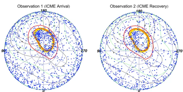
Figure 3. System III (S3) coordinate projections onto Jupiter’s geographic north pole (plot center) for the (left) first observation, during which the ICME arrived at Jupiter, and the (right) second observation, 1.2 days later. Lines of constant Jovian S3 longitude radiate outward from the pole, increasing clockwise in increments of 30∘from 0∘at the bottom of the projection. Concentric dotted circles outward from the pole represent lines of 80∘, 70∘, 60∘, and 30∘ latitude. The alternate green and black contours indicate VIP4 model magnetic field strength in Gauss. The outer red oval is the Grodent et al. [2008] contour of Io’s footprint (5.8R_J). The inner red contour is the footprint for the 30R_Jfield line from Vogt et al. [2011] mapping using the Grodent et al. [2008] anomaly model. The thick orange contour is the average location of the UV main oval from two HST observation campaigns in 2007 [Nichols et al., 2009]. The projections show more X-ray events in the hot spot (160∘–180∘S3 longitude, 60∘–70∘latitude) during the first observation than the second. The events appear to spread from the hot spot into the region from 150∘to 160∘. More clearly identifiable is the bright change in emission in the Auroral Enhancement Quadrant (180∘–270∘S3 longitude, 55∘–90∘latitude). The distribution of this emission is not only enhanced in the main oval but also poleward of this and at lower latitudes near Io’s magnetic footprint.

3. North Pole Projections

Using the technique applied in Gladstone et al. [2002], Elsner et al. [2005], and Branduardi-Raymont et al. [2008], time-tagged Chandra X-ray events were reregistered into Jupiter’s System III (S3) (1965) spherical latitude-longitude coordinates centered on the rotation poles. Hence, a sky-projected disk of 1.01 RJwas used

for both observations (shown in the supporting information). It should be noted that when reregistering to S3 coordinates, events emitted close to the limb of the Chandra-facing disk will have larger spatial uncertainties because of the increased obliquity of the planet’s surface relative to the observer.

We estimated spatial uncertainties on events based on Chandra’s spatial resolution, by perturbing the Jupiter-centered disk by two pixels in the x and y directions, then reregistering the events into S3 coordinates. To identify the spatial distribution of auroral X-rays for the two observations, we present projections look-ing down onto the rotational north pole of Jupiter. Figure 3 shows these projections for both observations. Figure 4 shows counts versus latitude plots to quantify the latitudinal concentrations of X-rays. During these observations the south pole emission was obscured by the viewing geometry, so we focus on the north pole projections only.

We observe a range of differences in the spatial distribution of X-rays between the observations (Figures 3 and 4). A surprising difference is a broad bright auroral enhancement in the first observation between 180∘ and 270∘ longitude and above 60∘ latitude. The emission in this area is much dimmer in the second observa-tion. This enhancement is significantly spatially separated from the hot spot (S3 longitude: 160∘ –180∘, latitude 60∘ –70∘ [Gladstone et al., 2002; Elsner et al., 2005; Branduardi-Raymont et al., 2008]), where the brightest X-ray emission was previously observed. The region above 60∘ latitude and with longitudes 180∘ –270∘ features 201 ± 14 X-ray counts in the first observation compared to 76 ± 9 counts in the second.

(10)

Figure 4. Number of events in 5∘latitude bins during the ﬁrst (blue) and second (red) observations. (top) Hot Spot Quadrant with S3 longitudes 90∘–180∘. (bottom) Auroral Enhancement Quadrant with longitudes 180∘–270∘. For the Auroral Enhancement Quadrant, emission above 60∘latitude is up to 5 times brighter in the ﬁrst observation than the second. Error bars are calculated from Poisson statistics. At the time of maximum visibility, each quadrant above 60∘ latitude had a projected area of∼3% of the total observable Jovian disk.

Given the changing solar wind conditions throughout the observations (section 2) and our lack of knowledge concerning the processes governing both the hot spot and the auroral enhancement, we shall analyze the two separately. We refer to the 90∘ –180∘ longitude quadrant as the “Hot Spot Quadrant” (HSQ) and to the quadrant between 180∘ and 270∘ longitude as the “Auroral Enhancement Quadrant” (AEQ). However, we note that there is brightening across both quadrants and that this may be connected.

We focus first on the HSQ. For both observations, the majority of the auroral emission (above 60∘ latitude) occurs poleward of the 30 R_Jcontour (the inner red oval in Figure 3), indicating that the precipitating particles originate farther away from Jupiter than this. The whole region of the HSQ inside the 30 R_Jcontour contains 113 ± 11 counts in the first observation compared to 78 ± 9 counts in the second. Previously [Gladstone et al., 2002; Elsner et al., 2005], the hot spot was defined as located between 160∘ and 180∘ S3 longitude and 60∘ and 70∘ latitude, where we find 52 ± 7 counts in the first observation and 37 ± 6 counts in the second obser-vation. We find that the hot spot appears to spread out spatially in the first obserobser-vation. The outer edge of the hot spot (at longitudes 150∘ –160∘ and latitudes 55∘ –60∘) is where the greatest change occurs, with 55 ± 7 X-ray counts in the first observation compared to 28 ± 5 counts in the second. This changing emission occurs between the 30 R_Jcontour and the hot spot, in a region which during a 2007 Hubble Space Telescope (HST) observing campaign was where the poleward edge of the UV main oval was observed [Nichols et al., 2009]. The second observation appears to have its events much more concentrated in the previously defined hot spot. UV observations have shown that when solar wind compression regions onset, the UV auroras brighten in the “active region” close to this X-ray region, near noon and poleward of the main oval [Grodent et al., 2003; Nichols et al., 2007].

(11)

Journal of Geophysical Research: Space Physics

10.1002/2015JA021888

Figure 5. X-ray aurora lightcurves for the (top) ﬁrst and (bottom) second observations. Blue line: X-rays in the Hot Spot Quadrant (S3 longitude: 90–180∘). Red line: X-rays in the Auroral Enhancement Quadrant (S3 longitude: 180–270∘). The lightcurves were generated by placing events above 60∘latitude in S3 coordinates into 1 min bins. These were then shifted to account for Jupiter-Earth light travel time of 34 min (UT 34 min). The subsolar longitude at the time of the observations is indicated along the top of each plot. The green vertical dashed line indicates the onset of the brightest burst of non-Io decametric emission in the STEREO A data. The projected area of each quadrant (as a percentage of the total area of Jupiter) is indicated by the blue (HSQ) and red (AEQ) dashed lines. At the point of maximum visibility each quadrant above 60∘latitude takes up a projected area that is∼3% of the total observable Jovian disk.

For the Auroral Enhancement Quadrant, the first observation displays additional bright features with respect to the second. The difference is most evident in Figure 4, which shows the emission is up to a factor of 5 brighter across all latitude regions from 55∘ to 85∘ during the first observation relative to the second. Additionally, Figure 4 shows that in the first observation the levels of emission observed in the AEQ are com-parable to those in the same latitude range in the HSQ. Comparing the changes in counts for the HSQ and AEQ could suggest that the HSQ is less sensitive to the ICME than the AEQ. Alternatively, it could suggest that the changes the ICME drives in the X-ray aurora develop with time or with varying solar wind parameters—as Jupiter rotates, the HSQ is visible first and the AEQ rotates into view slightly later (Figure 5).

One other aspect to note from the HSQ latitude-count plot (Figure 4) is that there appears to be increased emission from the disk/equatorial region. This suggests the presence of increased solar X-ray flux, which is flu-oresced and elastically scattered in the Jovian atmosphere. The occurrence of a solar flare at a time consistent with the increase is confirmed by inspection of GOES X-ray lightcurves (see supporting information). Analysis of the polar projections for discrete energy regimes section 6 shows that the flare is not a significant contribut-ing factor for the increased auroral emission, ensurcontribut-ing the validity of the changcontribut-ing auroral activity. We note that this solar flare is a distinct event from the ICME and directly introduces additional solar X-ray photons to the Jovian disk, while the ICME introduces X-rays indirectly.

(12)

4. Auroral X-Ray Lightcurves

To generate the auroral X-ray lightcurves, we took those events which occurred above S3 latitudes of 60∘ in the polar projections (section 3) and placed them into 1 min time bins. We then shifted the lightcurves to account for Jupiter-Earth light travel time. During the ﬁrst observation, the X-ray emission was brighter and more vari-able with multiple enhancements that contain twice as many counts as similar enhancements in the second observation. To distinguish between variation in emission from the HSQ and the AEQ, we produced separate lightcurves for each quadrant (Figure 5). To help identify any local time dependencies, we also indicate the subsolar longitude (SSL) corresponding to the timing of the observations.

Figure 5 shows that the ﬁrst half of each observation was dominated by the hot spot. In the ﬁrst observation, the hot spot became visible shortly before DOY 276.04 and 80∘ SSL and the counts increased by up to a factor of 6, from ∼4 c/ks to peaks of 19–27 c/ks. For the second observation the hot spot appeared on the face before DOY 277.7 and the counts increased by up to a factor of 4.5, from 4 to 18 c/ks.

The AEQ shows the most striking difference between the lightcurves. The second observation was generally quiet, with ∼3–5 c/ks, with the exception of a single peak containing 9 c/ks at 277.93. In contrast, the first observation contained a prominent single peak of 33 c/ks at DOY 276.24, which lasted 15–25 min and was higher than the peak emission from the hot spot. Prior to the peak, there was a gradual increase from DOY 276.2 to 276.22. After the peak there was an abrupt drop to 17 c/ks and then a gradual decrease for 0.1 DOY afterward, as the region rotated out of view. From the moment the region began to be observable it was emitting 6 c/ks, while in the second observation it emitted only 1–2 c/ks, suggesting that the whole region was brighter throughout the first observation.

The peak of the enhancement occurred 1–1.5 h before the non-Io decametric radio burst at DOY ∼276.3 (indicated in Figure 5 by the dashed line). We also note that the fainter burst of non-Io decametric emission at DOY 276.2 coincides well with the preceding peak on the AEQ auroral lightcurve, suggesting a further possible connection between X-ray emission and non-Io decametric emission. The previously recognized con-nections between this non-Io decametric emission and forward shocks induced by ICMEs [Hess et al., 2012, 2014] suggest that the heightened X-ray emission is also likely to be directly connected with the ICME. We also detect periodicity in these lightcurves on the order of tens of minutes for both observations, and this is discussed and analyzed in section 8.

5. Auroral Spectra

5.1. Spectral Extraction and Modeling

For analysis of the Chandra spectra we divided Jupiter’s observed disk emission into three sections: a northern auroral zone, an equatorial region, and a southern auroral zone (see supporting information for regions selected). Given the limited visibility of the southern aurora, only the northern aurora is presented. Using the CIAO software package (provided by the Chandra X-ray Center), we followed the standard pro-cedures to extract spectra, which were then analyzed using the XSPEC package [Arnaud, 1996]. We applied a correction to the effective area to account for the increased energy thresholds applied within ACIS to circumvent optical light leaks through the OBFs (as discussed in section 2.1). To do this, we weighted ener-gies below 0.7 keV based on fitting for the signal degradation to E0102-72.3, which provided a best fit curve of 1 − Y ∗ (x − 0.7) ∗∗ 2 with Y = 0.50 and x = the energy of channel.

We again treated the HSQ and AEQ separately. To do this, we separated each observation into two halves based on the time at which the emission from the hot spot dimmed (Figure 5). The spectrum for the first (second) observation HSQ was produced at Jupiter from DOY 275.95 to 276.15 (277.6 to 277.8) UT, while the AEQ events occurred from DOY 276.15 to 276.35 (277.8 to 278) UT. The time intervals were selected to maxi-mize exposure times of the given quadrant, while minimizing contamination from the other. Figures 6a and 6b compare the HSQ spectra, and Figures 6c and 6d compare those from the AEQ, for the two observations. We fitted the spectra between 240 and 2000 eV, with a combination of lines with half widths fixed at 20 eV. This produced two challenges. First, the low count rates and large error bars produced unrealistically low reduced𝜒2_{values of 0.4–0.6 (for 105–111 degrees of freedom). Second, Chandra’s spectral resolution and}

energy cutoff at ∼210 eV lead us to ignore the region from 210 to 250 eV, since the sharp drop in counts in this region inhibited good fitting. Table 1 and Figure 6 show the best fits.

(13)

Journal of Geophysical Research: Space Physics

10.1002/2015JA021888

Figure 6. The northern auroral zone spectra for the (a, c) first and (b, d) second observations. The Hot Spot Quadrant spectra are in Figures 6a and 6b, while the Auroral Enhancement Quadrant spectra are in Figures 6c and 6d. The data have been fitted with a combination of lines with half widths fixed at 20 eV.

5.2. Spectral Analysis

Inspecting the HSQ spectra (Figures 6a and 6b) ﬁrst, both observations featured a large peak between 250 and 350eV, which could be from sulfur and/or carbon ions.

Between 500 and 900 eV there was a range of oxygen lines. Both observations contained lines near 600 eV and between 700 and 730 eV, which are likely to be from O VII and possibly also O VIII transitions. The first obser-vation showed an additional spectral line at ∼ 860 eV, which could have either been from O VIII transitions or evidence for solar X-ray scattering from the disk. While the best fit model contained only one line at 730 eV, we were also able to obtain similar reduced𝜒2_{values by fitting two lines at ∼700 eV (O VII) and ∼780 eV}

(O VIII), which may suggest that the additional line at 860 eV was also an O VIII transition.

As mentioned in section 3, a solar X-ray ﬂare reached Jupiter during the time covered by this spectrum (see supporting information for further details) and may have imprinted solar lines onto the spectrum. The addi-tional emission above 700 eV could have been from Fe XVII, Fe XXI, or Ne X solar photons or a combination of oxygen and solar photons. We also observed a magnesium (Mg XI) line in the spectra near 1350 eV, which would be expected from a solar ﬂare [Branduardi-Raymont et al., 2007a; Bhardwaj et al., 2005, 2006]. These solar features are absent or much less relevant in the AEQ and throughout the second observation.

For the AEQ, the difference between the spectra of the two observations is clear (Figures 6c and 6d). The first shows a prominent peak between 200 and 300 eV that appears to be 3–4 times higher for the first observation than the second. We were unable to model this accurately because of the low-energy cutoff and low spectral resolution, meaning that comparing fluxes and differentiating between sulfur and carbon was not possible. Between 300 and 500 eV there are additional transitions of carbon or sulfur which do not appear in the HSQ spectra or the AEQ spectrum for the second observation.

The morphology of the AEQ spectrum between 380 and 700 eV is particularly interesting. The emission between 550 and 600 eV is mostly O VII, and the line appeared to be asymmetric, with a sharp decline after 600 eV, which led the ﬁt to underestimate the ﬂux for this line in Table 1. This region of the spectrum is similar to that of comets LINEAR S4 and McNaught-Hartley displayed by Elsner et al. [2005]. This similarity to cometary solar wind charge exchange spectra could suggest a solar wind origin for some of the precipitating ions.

(14)

Table 1. Best Fit Parameters for the 0.24–2 keV Spectra and Closest Known Ion Rest Frame Lines [Elsner et al., 2005; Kharchenko et al., 2008; Branduardi-Raymont et al., 2007b]a

Best Fit Line (eV) Flux (photons/cm2_/s) _{Known Ion Rest Frame Energies}

First Observation Hot Spot Quadrant—Reduced𝜒2_∼_{0.45 (105 Degrees of Freedom)}

310±10 5±1×10−4 _{S VI–X (260–291; 314; 316 eV) or C V (299; 304–308 eV)} 595±20 1.5±0.5×10−5 _{O VII (561; 568; 574 eV)}

730±35 6.5±3×10−6 _{O VII (698–713 eV) or O VIII (774 eV)} 860±30 4.5±1.5×10−6 _{O VIII (836 eV) or Solar Fe XVII (812; 826 eV)} 990±60 1.5±1×10−6 _{Solar Ne X + Fe XXI (}_∼_{1000 eV)} 1140±85 9±6×10−7 _{Solar Ne X + Fe XXI (}_∼_{1000 eV)}

1375±60 1±0.5×10−7 _{Solar Mg XI (1350 eV)}

Second Observation Hot Spot Quadrant—Reduced_𝜒2_∼_{0.4 (111 Degrees of Freedom)}

310±10 4.5±1×10−4 _{S VI–X (260-291 eV) or C V (299; 304–308 eV)} 610±50 9±5×10−6 _{O VII (561; 568;574 eV) or O VIII (654 eV)}

700±35 8.5±5.5×10−6 _{O VII (698–713 eV)}

925±25 4±1 x 10−6 _{Solar Ne X + Fe XXI (}_∼_{1000 eV)}

First Observation Aurora Enhancement Quadrant—Reduced𝜒2∼0.6 (109 Degrees of Freedom)

305+10₋₁₀₀ 3±2×10−4 _{S VI–X (260–291 eV) or C V (299; 304–308 eV)} 390±60 4.5±3×10−5 _{S IX- S XIV (336–348; 380 eV) or C V–VI (354–378 eV)} 590±15 1.5±0.5×10−5 _{O VII (561; 568; 574 eV)}

775±20 7±2×10−6 _{O VIII (774 eV)}

915±65 1.5±2×10−6 _{Solar Ne X + Fe XXI (}_∼_{1000 eV)}

Second Observation Aurora Enhancement Quadrant—Reduced_𝜒2_∼_{0.55 (111 Degrees of Freedom)} 310±10 2±1×10−4 _{S VI–X (260–291 eV) or C V (299; 304–308 eV)} 645±40 7±2.5×10−6 _{O VII (665 eV) or O VIII (654 eV; 698–713 eV)} 875±60 2±1×10−6 _{O VIII (836 eV) or Fe XXI + Ne X (}_∼_{1000 eV)} 1095±65 1±0.5×10−6 _{Solar Ne X + Fe XXI (}_∼_{1000 eV)}

a_{Line Half Widths Were Held Constant at 20 eV.}

The 775 eV line appeared to be a good match for the O VIII transition. GOES data (supporting information) shows that the heightened solar X-ray flux from the first half of the observation was returning to normal at these times, so it is unlikely that solar photons caused the 700–900 eV morphology in this spectrum. For the AEQ in the second observation, the spectrum is best fitted by a set of low flux sulfur/carbon and oxygen lines. Some of this emission may be contamination from the HSQ, which was still partially visible during these times.

6. Connecting Spatial and Spectral Features

Given that Chandra’s spectral resolution is insufficient to definitively separate between the spectral lines of carbon and sulfur ions, we now examine the auroral morphology in different energy bands. By combining this with magnetic field mapping, we tried to establish the magnetospheric or solar wind origins for specific ion species. To do this, we binned X-rays into four broad energy bins for carbon/sulfur, oxygen, solar X-ray lines, and hard X-rays. We then plotted the polar projections for each energy range separately. The specific energy ranges were chosen based on (a) the ease with which regions could be differentiated in the spectrum, (b) the relevant spectral lines for different species [Elsner et al., 2005], (c) Chandra’s energy resolution limitations, and (d) by considering the solar X-ray lines from the equatorial region spectrum.

We estimated the carbon or sulfur emission from the spectra between ∼200 and 500 eV. We found that pho-tons below 300 eV mapped almost exclusively to the auroral zone, with very little disk component (Figure 7), so we included these photons in our analysis. The oxygen emission was deﬁned by the band ∼500–800 eV from spectral ﬁtting of strong O VII and O VIII lines [Branduardi-Raymont et al., 2004, 2007b; Elsner et al., 2005].

(15)

Journal of Geophysical Research: Space Physics

10.1002/2015JA021888

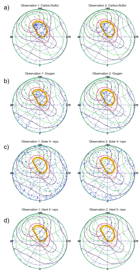
Figure 7. Comparisons of north pole S3 projections for discrete energy ranges for the (left column) ﬁrst and (right column) second observations. From top to bottom the energy ranges are (a) 200–500 eV (carbon/sulfur ion lines), (b) 500–800 eV (oxygen ion lines), (c) 800–1500 eV (dominated by ﬂuoresced and scattered solar photons), and (d) 1500–5000 eV (hard X-ray bremsstrahlung radiation from electrons). For further plot details see Figure 3.

(16)

Figure 8. Latitude-count plots for 5∘latitude bins. Comparisons of the (top row) 200–500 eV carbon/sulfur emission or (bottom row) 500–800 eV oxygen emission between the ﬁrst observation (blue line) and second observation (red line). The (left column) Hot Spot Quadrant and (right column) Auroral Enhancement Quadrant are treated separately. At the time of maximum visibility, each quadrant had a projected area of∼3% of the total observable Jovian disk.

We considered the ∼800–1500 eV emission to come from ﬂuoresced or scattered solar photons because this energy range contains the peak of the disk spectrum [Bhardwaj et al., 2005, 2006; Branduardi-Raymont et al., 2007a]. It should be noted that some O VIII lines from completely stripped oxygen [Elsner et al., 2005] also fall in this energy range and may contribute some of the observed auroral emission. Finally, we consider 1500–5000 eV emission to be hard X-rays from precipitating electrons generating bremsstrahlung radiation [Branduardi-Raymont et al., 2007b, 2008].

We look first at the polar projections of 200–500 eV carbon/sulfur X-ray events (Figure 7a) and find that for both observations almost all emission originated in the aurora, with very little equatorial emission. This confirms that the changing emission in this part of the spectra was unrelated to solar flares. We find that carbon/sulfur is the source of the brightening on the edge of the hot spot, between 150∘ and 160∘ S3 longi-tude (introduced in section 3). This emission lies in a region which during the 2007 HST observations [Nichols et al., 2009] featured the poleward edge of the UV main oval.

In the AEQ, for the first observation we find a large number of carbon/sulfur events between the Io footprint (∼5.8 RJ) and both the UV main oval and 30 RJcontour. For the AEQ, we also find ion emission poleward of

the 30 RJcontour. This is unexpected, since previous observations showed that the majority of ion emission

originated in the Hot Spot Quadrant. Emission from carbon/sulfur in the AEQ is largely absent from the second observation.

For the 500–800 eV oxygen emission (Figure 7b), events are also concentrated into the auroral zone. In the ﬁrst observation, the events occur poleward of the 30 RJcontour and the main oval reference contour in both

the HSQ and AEQ, while in the second observation the auroral events are almost solely concentrated into the hot spot. Comparing the oxygen with the carbon/sulfur emission, we ﬁnd that where there is some carbon/sulfur emission closer to the polar edge of the 30 RJcontour, the oxygen emission generally originates

poleward of this carbon-/sulfur-dominated emission region and appears to be more diﬀusely distributed across the entire polar region.

(17)

Journal of Geophysical Research: Space Physics

10.1002/2015JA021888

Figure 7c shows the 800–1500 eV emission, dominated by solar photons, distributed across the disk, and not concentrated into the aurora, as expected. The hard X-rays (Figure 7d) cluster in two regions parallel with the 30 RJcontour in the ﬁrst observation and are less prevalent in the second.

Figure 8 shows carbon/sulfur and oxygen latitude-count plots: the change between observations in carbon/sulfur emission is similar in both quadrants, while oxygen emission stays almost constant in the HSQ but changes by a factor of 3 in the AEQ. This diﬀering behavior and mapping for carbon/sulfur emission and oxygen emission may suggest diﬀerent sources for each.

7. Local Time Variation: Noon-Binned Projections and Magnetosphere Mapping

The configuration of Jupiter’s magnetosphere will evolve throughout the observations. As Jupiter rotates, a specific S3 longitude-latitude auroral position will map to changing magnetospheric local time sources. To identify how this rotation, and the associated change in local time, changes the X-ray aurora and to identify possible magnetospheric local time origins for features, we mapped the magnetosphere footprint configu-ration at distinct subsolar longitudes (SSL). The SSL indicates which Jovian S3 longitude is directly facing the Sun at a given time—the location of noon.

To do this, we subdivided each 11 h observation into 50 min time bins. For each time bin, we compared the S3 coordinates of auroral spatial and spectral features with their mapped source regions using the Jovian magnetosphere-ionosphere model from Vogt et al. [2011].

The Vogt model maps contours of constant radial distance from the magnetic equator to the ionosphere by ensuring that magnetic ﬂux at the equator equals magnetic ﬂux in the ionosphere. This enabled us to map ionospheric footprints to their equatorial magnetospheric origins up to 150 R_Jfrom the planet, where the VIP4 model [Connerney et al., 1998] used for previous Jupiter X-ray observations was limited to 30 RJ[Gladstone

et al., 2002; Elsner et al., 2005; Branduardi-Raymont et al., 2008]. The Vogt model accounts for the bend-back of Jupiter’s field lines, in order to map field lines to their magnetospheric local time origins. For instance, this could inform us that a specific ionospheric footprint maps to an equatorial magnetospheric source 50 RJfrom

the planet at dawn magnetospheric local time.

Using NASA Jet Propulsion Laboratory Horizons ephemerides data, we chose the start and end times of 50 min X-ray bins to coincide with 30∘ increments of SSL. X-rays emitted at times when the SSL was 15∘ –45∘ were compared to the Vogt et al. [2011] mapping model at SSL 30∘ to identify the sources for these X-rays and so on for each 30∘ SSL increment.

Joy et al. [2002] showed that the magnetopause location of Jupiter is bimodal. During periods of low solar wind dynamic pressure, the nose of the magnetopause standoﬀ is expected to reach ∼92 RJ(an expanded

magnetosphere), while for the high dynamic pressure periods, it will be as close as ∼63 RJ(a compressed

magnetosphere). Vogt et al. [2011] account for these two diﬀerent possible magnetopause standoﬀ distances by moving the magnetopause location based on the measured distances of Joy et al. [2002].

The plotted projections in Figures 9–11 show the expanded magnetosphere mapping of Vogt et al. [2011]. The magnetopause is indicated by a thick purple contour. Jupiter’s closed magnetic ﬁeld lines map to lati-tudes equatorward of the magnetopause mapping. Toward noon (at the nose of the magnetopause), these closed ﬁeld lines are shown as contours from 15 RJ(red contour) to 95 RJ(green contour), in increments of

5 RJ. For the compressed magnetosphere (Figure 12) closed ﬁeld line contours at the nose of the

magneto-sphere extend only as far as 65 RJ (yellow contour). In the Jovian tail we mapped closed ﬁeld contours up

to 150 RJ. X-ray emission that maps to closed contours is likely to be produced by precipitating particles on

closed ﬁeld lines originating in Jupiter’s magnetosphere. X-ray emission that maps poleward of the magne-topause, to the region absent of contours, is from precipitating particles that are more likely to be on open ﬁeld lines.

Since Jupiter was close to opposition, the SSL and subobserver longitude were only ∼6∘ separated, so that the noon position on the planet was close to the center of the observed disk. This means that counts originating near the limb of the Chandra-facing disk are easily identiﬁable on the time-binned projections and their larger uncertainties can be accounted for in the context of the magnetic footprint at that moment.

Analyzing the SSL-binned polar projections with Vogt mapping revealed previously unreported relationships. First, for both the expanded and compressed magnetospheres we ﬁnd emission that mapped to the open

(18)

Figure 9. S3 polar projections showing X-ray emission coinciding with speciﬁc subsolar longitudes (SSLs). Each plot shows emission that occurred at times when the SSL was±15∘from the SSL stated (120∘in this case). The Sun’s direction (noon) lies along the red arrow, with dawn 90∘clockwise from this and dusk 90∘anticlockwise. A Vogt et al. [2011] mapping using a Grodent Anomaly Model [Grodent et al., 2008], assuming an expanded magnetosphere, is plotted onto this polar projection. The plot shows closed ﬁeld lines increasing in increments of 5R_Jfrom the 15R_Jcontour (red), through 50–80R_Jcontours (yellow), to the last closed contour at the nose of an expanded magnetosphere 90R_J

(inner green contour). Green contours map to 95–150R_J. The thick purple contour indicates the predicted open-closed ﬁeld line boundary. Regions poleward of this and absent of contours indicate regions mapping to open ﬁeld lines. Events occurring close to the noon position have uncertainties in their spatial position of∼5∘latitude-longitude, while those occurring closer to dawn or dusk originate on the limb and have uncertainties of∼10∘–20∘latitude-longitude. Emission is color coded: carbon/sulfur photons (red), oxygen photons (blue), solar X-rays photons (grey), and hard X-rays from electrons (green). Carbon/sulfur emission can be found mostly on contours mapping to 50–90RJand also

clustered in the open ﬁeld line region. Oxygen emission is mostly on contours of 70–120RJand in open ﬁeld line

regions. The hard X-rays from electrons can be found clustered on the dawn edge of the projection.

ﬁeld lines and also emission that mapped to the magnetosphere, suggesting that both could be sources for Jovian auroral X-rays. For the expanded model (Figures 10 and 11) the majority of the emission originated on the magnetosphere side of the magnetopause, while for the compressed model (Figure 12) the majority of emission originated on open ﬁeld lines.

This may be particularly noteworthy for the ICME arrival observation. During this observation a compres-sion may be expected to shift the magnetopause boundary from ∼92 RJ to ∼63 RJ [Joy et al., 2002]. It

is this region mapping to 60–90 RJ, across which the magnetopause would be compressed, which

con-tained the hot spot expansion during the ﬁrst observation and where we observed increased X-ray emission. The closeness of the emission to the magnetopause, our spatial uncertainties, and our uncertainty in the choice of expanded or compressed magnetosphere inhibited us from precisely quantifying the relative impor-tance of a solar wind versus a magnetospheric origin. The Vogt et al. [2011] models showed, however, that the majority of X-ray-producing ions originate beyond 60 R_J.

Figures 10 and 11 also show, and particularly for the first observation, that emission clusters along the open-closed field line boundary and seems to move with SSL, suggesting a local time dependence and rela-tionship with processes in this region. The emission seems to follow the region where field lines would be opening or where closed field lines occur in the afternoon to dusk flank.

7.1. Noon-Binned Hot Spot Projections

For our observations, we considered the hot spot to be above 60∘ latitude and between S3 longitudes 150∘ –180∘. We found for both observations that the hot spot had a strong local time dependence and

(19)

emit-Journal of Geophysical Research: Space Physics

10.1002/2015JA021888

Figure 10. S3 polar projections of the ﬁrst observation, binned based on subsolar longitude (SSL). Vogt et al. [2011] expanded magnetosphere models are plotted onto the polar projections. Throughout the observation, emission appears to exhibit a local time dependence and may follow the open-closed ﬁeld line boundary. The time bins at 270∘and 300∘SSL show the auroral enhancement event. Each dot is an X-ray photon. For further plot details see Figure 9.

ted 78 of 100 X-rays (first observation) and 51 of 74 X-rays (second observation) before noon (165∘ SSL). After this time the hot spot became dimmer, despite the region remaining observable on the Jovian disk for several hours after this. Looking at the development of the magnetic field leading up to 165∘ SSL (Figure 13), we found that the majority of the hot spot emission originated on the dayside of Jupiter, with magnetospheric local times (MLTs) between 10:30 and 18:00. Later in the observation, when the field lines that mapped to MLTs after 18:00 were still observable in the hot spot, we found significantly less emission from the region. Having found that the hot spot emission occurred predominantly in the projections 90∘ –150∘ SSL (Figures 10 and 11) (prior to mapping to MLTs of 18:00), we analyzed these more closely. For the 90∘ SSL projection,

(20)

Figure 11. S3 polar projections of the second observation, binned based on subsolar longitude (SSL), with Vogt et al. [2011] expanded magnetosphere models. Each dot is an X-ray photon. For further plot details see Figure 9.

the hot spot was close to the limb of the disk, so there was a large uncertainty of 10∘ –20∘ in the X-ray coordinates. Based on this, we focused our attention on projections of 120∘ and 150∘ SSL (Figures 12 and 13), where the uncertainty was closer to 5∘ latitude-longitude.

Considering the first observation 120∘ SSL projection (Figures 12 and 13), in the region of 150∘ –170∘ longi-tude and 55∘ –80∘ latilongi-tude, carbon or sulfur (red) emission and oxygen (blue) emission occurred along the field line contours. For the compressed magnetosphere, both carbon/sulfur and oxygen ions originated along the open edge of the open-closed field line boundary, while for the expanded magnetosphere the carbon/sulfur ions originated on closed field lines. Accounting for spatial uncertainties, the carbon/sulfur events originated between 50 and 90 RJ (yellow-green contours) and on open field lines, while the oxygen ions originated

(21)

Journal of Geophysical Research: Space Physics

10.1002/2015JA021888

Figure 12. Subsolar longitude (SSL) binned polar projections comparing (left column) compressed and (right column) expanded magnetosphere models for the hot spot during the ﬁrst observation. Projections for SSL of (top row) 120∘, (middle row) 150∘, and (bottom row) 210∘are shown. The models use Joy et al. [2002] measurements of the magnetopause distance. The compressed model uses a noon magnetopause at 63RJ, while the expanded model

assumes a noon magnetopause at 92RJ. The ﬁeld lines increase in increments of 5RJfrom the outer contour of 15RJ

(red), to the ﬁnal closed inner contour of 65 (yellow—Figure 12 (left column)) or 95 (green—Figure 12 (right column)). For color coding and plot details see Figure 9.

poleward of this between 70 and 120 RJ(green contours) and also on open ﬁeld lines. The emission was weaker

in the second observation for this SSL projection (Figure 13).

For the 150∘ SSL projection, both observations (Figure 13) contained clustering of X-rays between 160 and 170∘ S3 longitude and 60 and 70∘ latitude from the afternoon-dusk ﬂank of the magnetosphere [Vogt et al., 2011]. Given that the time binning is broad (50 min) across 30∘ SSL, it is uncertain whether these ﬁeld lines were open or closed for most of this X-ray emission. Considering uncertainties in the spatial location,

(22)

Figure 13. Subsolar longitude (SSL) binned polar projections for the hot spot for the (left column) ﬁrst and (right column) second observations, using an expanded magnetosphere model for both. For color coding and details see Figure 9.

this region would map either to the solar wind or closed ﬁeld lines between 90 and 150 RJ. The similar source

in both 120∘ and 150∘ SSL may suggest that the processes are persistent.

Finally, inspecting the 210∘ SSL projection (Figure 13), we found that the hot spot contained very little emis-sion, despite remaining on the observable disk. The emission appeared to have followed those ﬁeld lines that mapped to MLT regions from 12:00 to 18:00 as Jupiter rotated, and we found emission in both the outer magnetosphere and on open ﬁeld lines in this area.

To reﬂect our spatial uncertainties, the timing spread of events and their broad spatial distribution in each region, we found a broad range of MLT sources for the emission. For the 120∘ and 150∘ SSL projection, most ion emission originated from magnetosphere locations with local times between 10:30 and 18:00. For the 210∘ SSL projection, events mapped to MLTs of 8:30–19:00 (Figure 13). However, we note that none

(23)

Journal of Geophysical Research: Space Physics

10.1002/2015JA021888

Figure 14. Subsolar longitude (SSL) binned polar projections for the auroral enhancement for the (left column) ﬁrst and (right column) second observations, using the expanded magnetosphere model for both. The auroral enhancement occurs in the 270∘SSL plot. For color coding and plot details see Figure 9.

of these MLTs account for ion travel time from regions near the magnetopause to Jupiter’s pole. During this time, the magnetosphere will rotate and so the origins for the particles may be at earlier MLTs than we have suggested. Without knowing the location of the energization region for the ions, it is diﬃcult to quantify this time lag.

7.2. Noon-Binned Auroral Enhancement Projections

To identify the source(s) and development of the auroral enhancement, we focus on the 240∘, 270∘, and 300∘ SSL projections (Figure 14). Unfortunately, the auroral region had just begun to rotate out of view at this time, so a lot of the brightening occurred close to the limb of the disk, meaning that there were uncertainties of 10∘ –20∘ on the S3 coordinates of many X-rays.

The 270∘ SSL projection, when the auroral enhancement occurred, contained a broad spread of emission from closed lines in the outer magnetosphere and ﬁeld lines that were open to the solar wind. This showed both