with Applications to Industrial Inspection
Classification, Segmentation and Morphological extensions
Doctoral Dissertation submitted to the
Faculty of Informatics of the Università della Svizzera Italiana in partial fulfillment of the requirements for the degree of
Doctor of Philosophy
presented by
Jonathan Masci
under the supervision of
Prof. Jürgen Schmidhuber
Prof. Michael Bronstein University of Lugano
Prof. Illia Horenko University of Lugano
Prof. Hugues Talbot Université Paris-Est, ESIEE
Prof. Yann LeCun Courant Institute of Mathematical Sciences, New York University Director of AI Research, Facebook
Dissertation accepted on 27 March 2014
Research Advisor PhD Program Director
Prof. Jürgen Schmidhuber The PhD program Director pro tempore
mitted previously, in whole or in part, to qualify for any other academic award; and the content of the thesis is the result of work which has been carried out since the official commencement date of the approved research program.
Jonathan Masci
Lugano, 27 March 2014
Learning features for object detection and recognition with deep learning has received increasing attention in the past several years and recently attained widespread popularity.
In this PhD thesis we investigate its applications to the automatic surface inspection system of our industrial partner ArcelorMittal, for classification and segmentation problems. Currently employed algorithms, in fact, use fixed fea-ture extractors which are hard to tune and require extensive prior-knowledge.
Our work, instead, focuses on learnable systems that can be used to improve recognition and detection without requiring hard to obtain task-specific domain knowledge.
For image classification we propose extensions to max-pooling convolutional networks, so that they can be applied to solve the general defect classification problem via a new pooling and feature encoding schemes.
State-of-the-art deep learning algorithms for object detection/segmentation have reached outstanding performance given high-quality annotated data. Un-fortunately, they do not meet the required processing speeds of steel industry. We propose an architecture that does not suffer the same computational bottle-neck (1500-fold speed-up) while retaining equal performance.
To further advance the field we study the learning of morphological oper-ators, largely used in industry. Only few attempts have been proposed in the literature, but no approach has ever considered the problem in its generality because of its hard formulation. We tackle it from a different perspective and introduce a learnable framework which seamlessly integrates morphological op-erators; hence bringing these powerful tools to deep learning for the first time.
Re-engineering an industrial system requires time. In order to deliver an im-mediate return we investigate metric learning problems to boost performance of currently used features. Our multimodal similarity sensitive hashing model scales well to web-scale datasets and, thanks to the binary representation, re-quires little storage and involves a cheap distance computation. It outperforms previous state-of-the-art approaches without requiring additional resources.
I would like to thank my advisor Prof. Jürgen Schmidhuber for his guidance and support during my work. I would also like to thank, with particular regards, Dr. Ueli Meier for having taught me how to be a good researcher and that I should never underestimate myself. Thanks also to Dr. Dan Ciresan without whom learning how to efficiently implement and use convnets would have took ages. I am grateful to all members of my institute, in particular to Varun Raj Kompella, Marijn Stollenga, Hung Ngo, Matt Luciw, Sohrob Kazerounian, Ru-pesh Srivastava, Alessandro Giusti and to all external collaborators I have had the honor and pleasure to work with. A special mention to Prof. Jesus Angulo and Dr. Gabriel Fricout for their valuable help and to Prof. Faustino Gomez for having taught me how improve my writing and presentation skills and for having spent his valuable time to review this manuscript. I would like to thank Prof. Michael Bronstein for the time and dedication demonstrated during our collaboration and finally all the reviewers who dedicated their valuable time to provide comments to improve this thesis.
Most importantly I would like to thank my family and my wife. Without their support I would have not been able to complete this PhD and it would have not had the same value.
Contents ix
List of Figures xiii
List of Tables xxi
1 Introduction 1
2 Background 7
2.1 Automatic Surface Inspection Systems . . . 8
2.2 Deep Learning for Vision. . . 12
2.2.1 Linear regression and multilayer perceptron . . . 14
2.2.2 Convolutional neural networks . . . 17
2.2.3 Learning strategies. . . 22
2.2.4 Preventing over-fitting . . . 25
2.3 Mathematical morphology. . . 31
2.3.1 Morphological operators . . . 32
2.3.2 Morphology in the steel industry . . . 39
2.4 Similarity based metric learning . . . 41
3 Classifying defects with MPCNN 47 3.1 Standard Features . . . 47 3.2 Dataset . . . 50 3.3 Experimental Setup . . . 52 3.4 Results. . . 54 3.4.1 Standard Features . . . 54 3.4.2 MPCNN . . . 54 3.4.3 Committee of classifiers. . . 56 ix
4 General steel defect recognition 57
4.1 Background. . . 58
4.1.1 Feature encoding algorithms. . . 60
4.1.2 Feature pooling . . . 61
4.2 Multi-Scale Pyramidal Pooling Network . . . 62
4.2.1 Pyramidal pooling Layer . . . 63
4.2.2 Multi-scale extraction . . . 65
4.2.3 Feature encoding layer . . . 66
4.3 Results. . . 67
4.3.1 Conventional Benchmarks . . . 68
4.3.2 Steel-Defects Industrial Benchmark . . . 73
5 Fast MPCNN image segmentation and detection 77 5.1 Fast Image Scanning . . . 80
5.2 Beyond patches: learning on full images . . . 84
5.2.1 The MaxPoolingFragment (MPF) layer . . . 85
5.2.2 Back–propagation through an MPF layer . . . 85
6 Application of MPCNN to steel segmentation and detection 89 6.1 Results on single-channel images . . . 89
6.1.1 Membrane Segmentation . . . 90
6.1.2 Single Defect Detection . . . 91
6.1.3 Multiple detections per image . . . 94
6.2 Results on multi-variate images . . . 96
7 Learning Morphological Operators using Counter-Harmonic Mean 103 7.1 Asymptotic morphology using Counter-Harmonic Mean . . . 104
7.2 Method . . . 105
7.3 Experiments . . . 107
7.3.1 Learning dilation and erosion . . . 108
7.3.2 Learning opening and closing . . . 109
7.3.3 Learning top-hat transform . . . 110
7.3.4 Learning denoising and image regularization . . . 112
8 Multimodal Similarity-Preserving Hashing 115 8.1 Similarity-Preserving Hashing . . . 117
8.1.1 Supervised single-modality similarity-preserving hashing . 118 8.1.2 Supervised cross-modality similarity-preserving hashing. . 120
8.2 Multimodal NN hashing . . . 120
8.3 Experiments . . . 124
8.3.1 CIFAR10 . . . 125
8.3.2 NUS. . . 126
8.3.3 Wiki. . . 132
9 Conclusions and Future Research 135 9.1 Learning compact key-point image descriptors . . . 135
9.2 Morphological Operators for Structured Pooling . . . 137
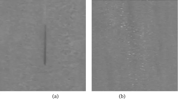
1.1 Sample images of two steel defects to illustrate the difficulties of the problem. On the left we have an extremely easy case, the de-fect is a vertical line, whereas on the right a challenging one, the defect is composed by the scattered spots. These images are taken from the current system and we clearly see that a big portion of the defect on the right is missing. . . 2
2.1 Illustrative example of a steel ASIS system processing pipeline. . 8
2.2 Illustrative example of a steel ASIS acquisition system. Source: ArcelorMittal. The steel is inspected from both sides by linear cameras and carefully chosen light sources. . . 9
2.3 Illustrative example of several models which made the history of deep learning. We go from a single layer perceptron to the mul-tilayer perceptron and reach the current state-of-the-art of deep networks which have many more layers of nonlinearity than con-ventional multilayer perceptrons. . . 15
2.4 A schematic representation of an MPCNN; the process flows left to right. Raw input pixel values are processed by a number of in-terleaved convolutional and max-pooling (MP) layers, which are trained to extract meaningful features. Several fully-connected layers (MLP) follow, which produce the final classification. . . 18
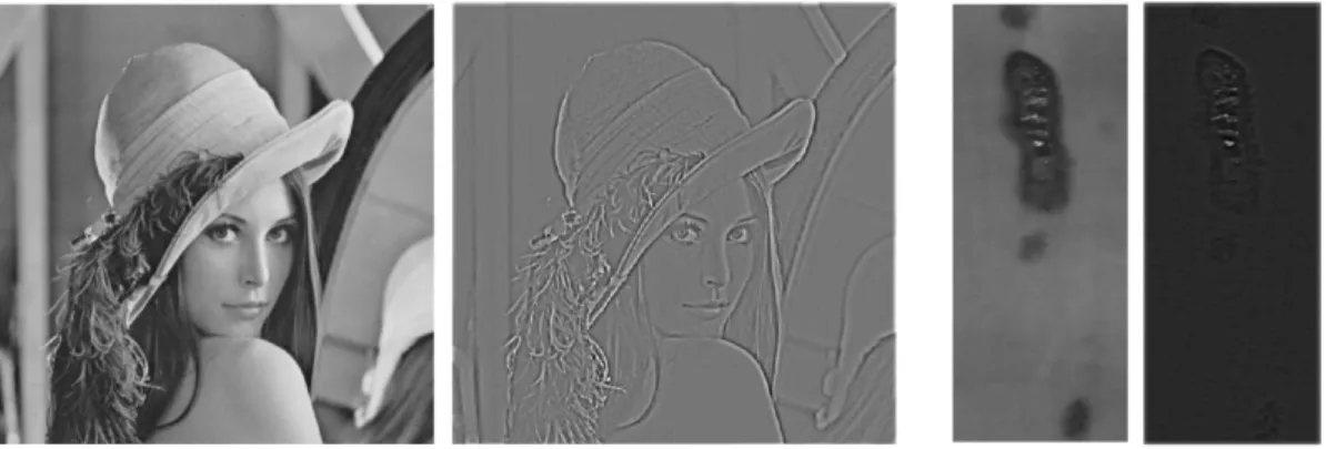
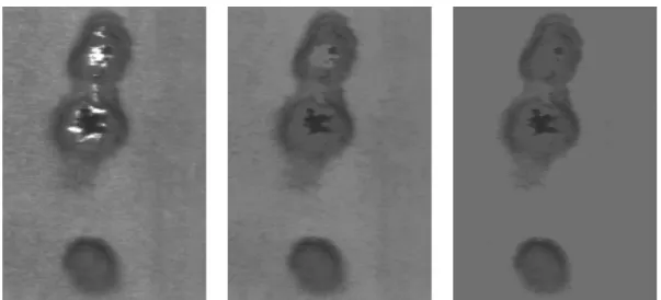
2.5 Examples of subtractive normalization on a conventional (left) and on a steel defect (right) image. . . 20
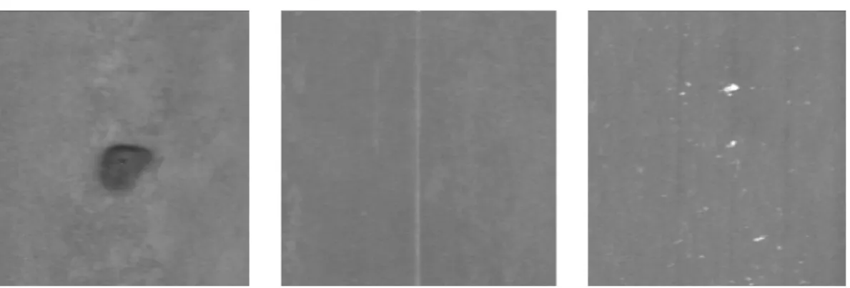
2.6 Examples of divisive normalization on a conventional (left) and on a steel defect (right) image. . . 20
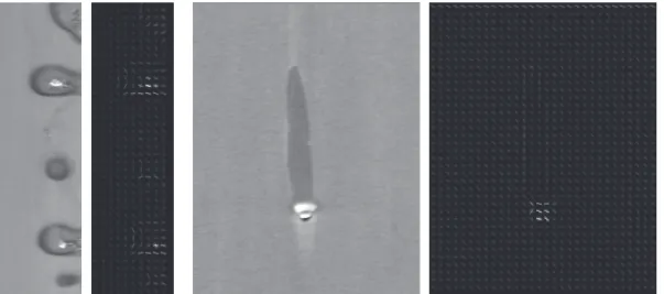
2.7 Examples of subtractive divisive normalization on a conventional (left) and on a steel defect (right) image. . . 22
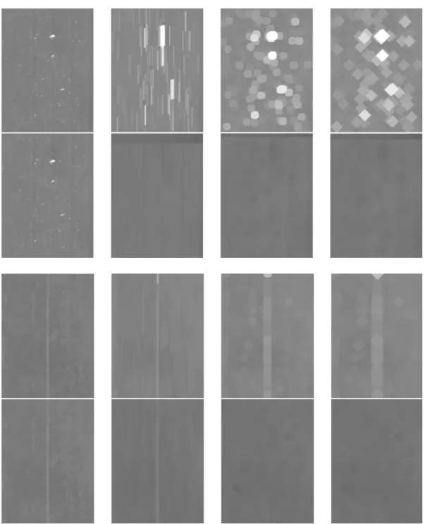
2.8 Examples of dilation and erosion with three different structuring elements. Leftmost column shows the original image, in this case we have a spot like defect and a vertically elongated one. Then from column 2–4 we have erosion (even rows) and dilation (odd rows) with respectively a vertical line of length 50, a disk of size 10 and a diamond of size 15. It is clear that with the dilation every bright structure that has at least a portion within the SE will be detected (white blobs); with the erosion the structure has to "fit" the SE in order to have a high response. . . 34
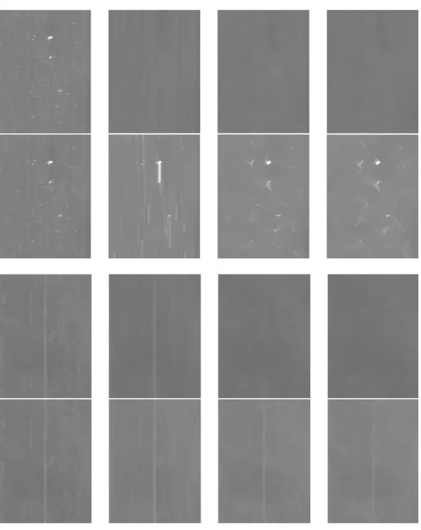
2.9 Examples of opening and closing with three different structuring elements as in Figure 2.8. Odd rows show the opening and even rows report the closing results. It is interesting to note the be-havior on the opening with a vertical structuring element (second column): in the case of the spot defect it is completely removed from the image as the structure is too small to fit entirely the morphological kernel; for the vertically elongated defect instead we have a response on the actual defect and remove partially the noisy background.. . . 36
2.10 Examples of opening by reconstruction using a disk structuring element of size 5 (central) and 50 (right). The original defected sample is shown on the left. Please note how the details are pre-served even which such a strong image simplification. . . 38
2.11 The three classes of defects for which a morphological detector based on residual operators needs to be designed. . . 39
2.12 Detection results with residual operators on the images shown in Figure 2.11 . . . 40
3.1 (a): A schematic representation of how a LBP descriptor is com-puted; (c) exemplar LBP image when applied to the steel defect image (b). . . 48
3.2 Visualization of HOG descriptors on industrial steel defect images. The detector is able to capture interesting points in the image and describes them with their gradient orientation. In cases where the background is highly textured, however, such an approach tends to fail. . . 49
3.4 Each point denotes the width and height of an image from the training set, histograms of the width and height distribution are also shown. It can be seen that most of the images are smaller than 150px in width and 200px in height. This distribution is used to empirically select the nominal size of the input images for the MPCNN. . . 51
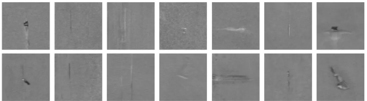
3.5 A sample from each of the seven defects in the dataset. First row: superior part of the strip; second row: inferior part of the strip. There is no correspondence between the two images for a given instance of the defect. . . 52
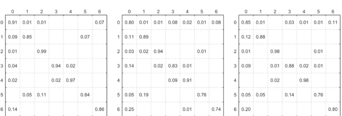
3.6 Confusion matrices for the best classifiers. Left: MPCNN, middle: PHOG, right: PHOG + MONO-LBP committee. Only on defect number two the classical features obtained a better result than that of the MPCNN. Also note the non marginal improvement of a committee w.r.t. the single best classifier. . . 56
4.1 Schematic representation of a MSPyrPool Network where histogram-like representations are extracted at two levels and at two scales. The first scale represents the output of the convolutional layer whereas the second scale is given by the output of a pooling (downsampling) layer. The resulting features are concatenated and used as input for the classification layer. . . 62
4.2 Pyramidal Pooling Layer. Features at each level l of the pyramid are pooled along l2 equally sized quadrants and the histogram-like representations are concatenated to form a feature vector. . . 64
4.3 The MLPdict layer used for feature encoding. Image responses of a network layer are reshaped to produce K dimensional feature vectors, where K represents the number of images in the layer. Each pixel descriptor is mapped into another representation of size K0 for which only the maxima value per row is preserved. . . 67
4.4 Some exemplar images from the MNIST digit recognition dataset. 69
4.5 Some exemplar images from the CUReT texture recognition dataset.
. . . 70
4.6 Some exemplar images from the Caltech101 texture recognition dataset. . . 72
4.7 Subset of images from the steel-defects benchmark showing the great difference in size among various samples. In this setting is not possible to resize the images to the same size, hence a MPCNN is not applicable to solve this task. . . 74
4.8 Two misclassified images for which the network inverted the cor-responding classes (off diagonal elements in the confusion ma-trix). This example clearly shows the extreme difficulty of this task. . . 75
5.1 Illustrative example of how much redundant computation there is when testing a MPCNN on a patch-by-patch basis. Similarly such situation is encountered also during training. Yellow and blue patches are input to the same MPCNN which computes twice the same intermediate results indicated by the diagonal stripes. When a max-pooling operation is applied, given its partial result it is possible to classify only the pixel indicated in the corresponding output; e.g. A for yellow and B for blue. . . 79
5.2 MPF layer for the 2× 2 pooling case. Top: Forward pass,
Frag-ments (0,0) and (1,1) share the same maximal element; Bottom Back–propagation pass where partial derivatives are pushed back to the previous layer in the hierarchy; the partial results of each
Fragmentare summed together. . . 86
5.3 Illustrative example of how subsequent convolutional layers of a MPF layer work. The same operation is applied to each output fragment; the gradient is the sum of the gradients of the fragments. 87
6.1 A slice of the test set segmented using SEGNN trained on full im-ages. The image on the right shows the probability of each pixel to be assigned to the background (white) or to the membrane (black). Please refer to text for the network architecture details. 91
6.2 A typical steel defect example for the marker detection problem. The marker, whose location is shown in the target image, needs to be detected and a flag must be raised when the input image contains it. We can see that segmentation is almost perfect, illus-trating the power of the proposed approach for industrial appli-cations. . . 93
6.3 Precision-Recall curves for the three methods on the bobine dataset. We clearly see that SEGNN has a much better precision for any recall value. Of particular interest is the good performance when recall is high as it means that less false positive alarms are raised. 95
6.4 A typical steel defect example from the coil dataset. This is a more challenging problem than the one of Sec. 6.1.2. Given the images in the first column we are asked to produce the ROI as indicated in the second column, the ground-truth data. SEGNN results, for these test images, are reported in the third column. The top-most result is almost perfect. For the second image from the top, the long vertical stripe of SEGNN, even if larger than desired, after a visual inspection makes lot of sense as it closely capture the defected region. . . 96
6.5 Signatures used for the multi-variate dataset generation. Note that target C and D are extremely difficult to discriminate, they have no relevant peaks or differences but belong indeed to two different defect classes. . . 97
6.6 Example images from the multi-variate synthetic dataset of steel defects. Note that the data has 23 channels, but only channels 1, 10 and 23 are plotted in RGB for illustrative purpose only. Target images, second and fourth column from the left, show the defect and its corresponding color coded class label. Each defect, such as the red one for example, can come in different shapes so that learning the shape of the object does not suffice to obtain good performance. The first and third columns show the images which compose the synthetic dataset. . . 98
6.7 Precision-Recall curves for the three methods on the multi-variate dataset for the detection task where the SEGNN detector outper-forms by a large margin its best competitor. Please note that SEGNN does not require any knowledge on the data whereas the Target Detector needs the signature of the defects. We implic-itly solve the related inverse problem of finding such signatures through learning the segmentation map, in our opinion a remark-able achievement of our model. . . 99
6.8 Precision-Recall curves for the three methods on the multi-variate dataset where class 4 is labeled as background. When the 23-channel raw signal is used SEGNN achieves almost perfect pre-cision at very high recall, contrary to other approaches which sharply decay. . . 101
7.1 Illustrative example of a PConv layer. The network here repre-sented can be used for learning dilation and erosion. In case of multiple convolutional kernels (i.e. multiple structuring elements in this setting) there will be a P for each one of them. This way it is possible to learn a richer set of operators. . . 107
7.2 Examples of learning a dilation with three different structuring elements. The target and net output are slightly smaller than the original image due to valid convolution. The obtained kernel
w(x) for each case is also depicted. . . . 109
7.3 Examples of learning an erosion with three different structuring elements along with the learned kernel w(x).. . . 110
7.4 Top: an example of learning a closing operator where a line of length 10 and orientation 45◦ is used. Bottom: opening with a square structuring element of size 5. The network closely matches the output and almost perfectly learns the structuring elements in both PConv layers. . . 111
7.5 Learning a top-hat transform. The defected input image has bright spots to be detected. The network performs almost perfectly on this challenging task. . . 112
7.6 Learning two top-hat transforms. On the left, bright spots need to be detected. On the right, a dark vertical line. The network performs almost perfectly in this challenging task. . . 112
7.7 Top: Binomial noise removal task. The learned nonlinear operator performs better than the hand-crafted one by a relative margin of ≈ 7.7%. Learning uses noisy and original images—there is no prior on the task. Bottom: Salt’n’pepper noise removal task. Even here, the learned operator performs better than the corresponding morphological one. . . 113
7.8 Total Variation (TV) task. The network has to learn to approxi-mate the TV output (target) by means of averaging two filtering pipelines. . . 114
8.1 Schematic representation of the coupled siamese network. There are two networks, one for each of the modalities, coupled by the loss function Lx y. . . 122
8.2 Unimodal retrieval on CIFAR dataset. Shown are top 10 matches to three different queries (marked in red) using different hash-ing method with codes of length 48. All NN methods are used in L2 configuration. CM-SSH, CM-NN and MM-NN were trained on multiple modalities, and used in this experiment for single modal-ity retrieval. . . 126
8.3 Example of GIST-HOG matching on CIFAR dataset. Shown are the original descriptors and their 48-bit MM-NN L2 hash codes. Red shows the bits that are different w.r.t. the query. . . 128
8.4 Precision-Recall curves for the cross-modal retrieval experiments on CIFAR10 (solid: HOG–GIST, dashed: GIST–HOG) and NUS (solid: Tag–Bof, dashed: Bof–Tag). . . 131
8.5 Example of text-based image retrieval on NUS dataset using mul-timodal hashing. Shown are top five image matches produced by CM-SSH (odd rows) and MM-NN (even rows) in response to three different textual queries. . . 132
8.6 Example of image annotation on the NUS dataset using multi-modal hashing. Shown are Tags returned for the image query on the left. Groundtruth tags are shown in green. . . 133
8.7 Cross-modal (Bof–Tags) retrieval on the NUS dataset. Shown are top five matches different image queries (marked in red), ranked according to Tags similarity using 64-bit MM-NN hash. . . 133
8.8 Cross-modal (Image–Text) retrieval on the Wiki dataset. Shown are top five matches different image queries (marked in red), ranked according to text similarity using 32-bit MM-NN hash. . . 134
9.1 Typical pipeline of feature descriptor construction, consisting of: affine-invariant region detection and canonization, ensuring ap-proximate invariance to view point transformations; linear filter-ing part (e.g. gradient computation in SIFT), ensurfilter-ing illumina-tion invariance; non-linear part (e.g. local direcillumina-tions histogram in SIFT). Hua et al. focused on tuning the parameters of the lin-ear and non-linlin-ear parts of SIFT. Strecha et al. added another binarization stage. . . 136
3.1 Detailed networks structure. The time per sample refers to the time required for a trained network to produce the class prediction. 54
3.2 Classification results for the several methods on the steel clas-sification dataset. Classical features show results as SVM/MLP. For MPCNN the best run is presented along with, in parenthesis, the mean performance and standard deviation among 5 different runs. RC indicates that the first convolutional layer performs a random projection, not trained. . . 55
4.1 Classification results for the MNIST benchmark. The MSPyrPool network is compared with other CNN-based approaches which do not use any input preprocessing. . . 69
4.2 Classification results for the CUReT benchmark. A conventional MPCNN is compared with our MSPyrPool network. We also show the relative improvement of a MLPDict encoding stage.. . . 71
4.3 Classification results for the Caltech101 benchmark. A MSPyr-Pool net without an encoding layer (MSPyrMSPyr-Pool1), with a linear (MSPyrPool2) and a nonlinear encoding layer (MSPyrPool3) are listed. . . 72
4.4 Classification results for the Steel-defect benchmark where MPCNN fail. Various classifiers, trained on conventional features, are com-pared with the MSPyrPool network which outperforms, by large margin, any classifier based on engineered features. . . 73
5.1 Theoretically required FLOPS for convolutional layers when seg-menting a 512× 512 image using patch-based (FLOPSl
patch) and
image-based (FLOPSl
image) approaches. . . 83
5.2 Speed for segmenting a 512× 512 image using the large net de-scribed inCiresan et al.[2012a]. . . 84
6.1 Comparison of training times for the Membrane dataset. The overhead for generating the transformed samples is also included in the overall computation. The relative speed-up of SEGNN is shown in parenthesis. . . 91
6.2 Detection error results of our efficient learning framework for MPCNN. Test evaluation times for a given image are also reported along with the patch-based evaluation with the same implemen-tation (e.g. Matlab). . . 93
6.3 Average Precision results for several models on the full steel coil detection problem. All methods work on the same support of 32× 32 pixels. . . 95
6.4 Average Precision results for several models on the multi-variate dataset. Every model has to detect any of the 4 possible defects out of the background. . . 99
6.5 Average Precision results for several models on the multi-variate dataset where Target D is considered as background. Please note that Target C and D are very similar and therefore discriminating between them makes this task extremely hard; the Target Detec-tor has a consistent drop in performance whereas our deep learn-ing approach suffers only a minor degradation.. . . 100
8.1 Summary of the experiments and datasets. . . 125
8.2 Unimodal training and retrieval experiment on the CIFAR10 dataset. NN hash was trained on single modality only. Performance is shown as mAP in %. . . 127
8.3 Unimodal and cross-modal retrieval experiment on the CIFAR10 dataset. All methods were trained using multimodal data. CCA produces Euclidean embeddings. Performance is shown as mAP in %. . . 127
8.4 Unimodal training and retrieval experiment on the NUS dataset. NN hash was trained on single modality only. Performance is shown as mAP@10/ mAP in %, (– indicates no convergence was reached). . . 129
8.5 Unimodal and cross-modal retrieval experiment on the NUS dataset. All methods were trained using multimodal data. CCA produces Euclidean embeddings. Performance is shown as mAP@10/ mAP in %. . . 130
8.6 Cross-modal retrieval experiment on the Wiki dataset using 32-bit hashes (L2 with 32 tanh units) and Euclidean embeddings from
Introduction
Recognizing and localizing objects is a crucial task in many computer vision, pattern recognition and industrial applications. If we look at the steel indus-try for example, a common application is to automatically detect defects in the material, based on camera images taken during the manufacturing process. Fig-ure 1.1-(a) shows an image of a piece of defective steel. In this context, the problem involves solving the two following tasks: (1) segment the defective re-gion from the background, and (2) classify the defect in the image, if any is present. These two tasks, while being at two different levels of abstraction, have common roots in feature extraction algorithms, which are able to describe the local or global structure of the input pixels by a vector of numbers, usually called a descriptor or, simply, feature.
Looking at Figure1.1-(a) one may be tempted to design an ad-hoc algorithm to perform the task. In fact, for this particular case, taking the horizontal im-age gradient, and applying a threshold will do just fine. However, looking at Figure 1.1-(b), where the defect is in the form of a constellation of tiny dots, it becomes clear that such a direct approach is not trivial for the general case, es-pecially when highly discriminative features are required so that efficient, linear classifiers can be used. The difficulty of this problem is mainly attributed to high intra-class variability (within the same class defects instances vary greatly) and inter-class variability (apparently similar defects belong to different classes). Of course, the same applies to general object recognition and detection. For ex-ample, in the case of digit recognition the same class is represented by a broad range of different instances, e.g. there are many ways to write a “3” and many of those ways make it hard to distinguish a “3” from an “8” or a “9”.
In the steel industry the process of hand-crafting features for real-time in-spection systems has matured over the years, achieving exceptional performance
(a) (b)
Figure 1.1. Sample images of two steel defects to illustrate the difficulties of the problem. On the left we have an extremely easy case, the defect is a vertical line, whereas on the right a challenging one, the defect is composed by the scattered spots. These images are taken from the current system and we clearly see that a big portion of the defect on the right is missing.
in many cases. Unfortunately, this is done by trial and error, which can take an enormous amount of time (e.g. current steel production systems are the result of more than 10 years of intense study), and seems to have already reached a plateau in terms of performance. Moreover, the modern steel industry moves quickly, so that the algorithms it uses to ensure quality must adapt at the same pace.
In particular, there are two ongoing developments which are problematic for the current engineered system: (1) demand for several highly textured steel grades is fast increasing, and (2) gray-level acquisition cameras, standard in actual systems, are being replaced by more sophisticated high-resolution cam-eras with infra-red, color and hyper-spectral sensors. The first requires a very large number of feature extractors to be generated because the number of de-fect classes increases rapidly as new grades of steel are introduced. Furthermore, these new grades tend to be much more refined so that it is a real challenge, even for an expert, to distinguish between defect types and between defect and back-ground due to the high intra-class variability as seen in Figure 1.1-(b): bright
spots vary greatly in intensity and size, and can be spread over areas of several shapes that can vary by orders of magnitude.
The second development raises the challenge of feature extraction to the next level because now it must be performed on multi-variate images where domain knowledge has not yet been consolidated. For example, most of state-of-the-art computer vision systems rely on engineered features, such as SIFT [Lowe,
2004], which completely disregard any color information, and consider only
a gray-level version of the input image. Even though there have been several attempts to extend these approaches to color (e.g. color-SIFT [Van De Sande
et al., 2010]), and more generally to multichannel images, they have shown
only marginal improvement on conventional vision tasks leaving the mainstream to their old-fashioned counterparts. While this may be reasonable for natural images, to some extent, it is not for steel – while a face can be recognized by its shape (using only edges) the only way to distinguish between many steel defects is to use additional spectra. In fact, certain defects are only visible in infra-red band.
The key limiting factor of all these hand-crafted approaches vis-a-vis these developments is that the features are fixed. For example, when we extract the SIFT descriptor from natural scenes or omni-directional images the same algo-rithm is used regardless of the different properties of these datasets (e.g. their probability distribution). Only expert knowledge, and extensive testing can de-termine which features perform best.
Given all these considerations, it has now become necessary to investigate alternatives to the standard engineered solutions that are easy to adapt and ex-tend. Machine learning, and in particular deep learning, has in the past few years shown itself capable of learning low- mid- and high-level features for
recogni-tion[Jarrett et al.,2009; Zeiler et al.,2011]. The main advantage comes from
the way deep learners compute features: multiple extraction stages (e.g. non-linear projections, neural networks) are chained together to form a deep archi-tecture that is trained such that complex features are created in a bottom-up (hierarchical) fashion from the input data. Images, for example, are first de-composed into basic components (e.g. edges), later combined into corners and crosses and finally into object parts[Zeiler et al.,2011;Zeiler and Fergus,2013b;
Simonyan et al.,2013].
This multi-layer approach is in sharp contrast to engineered approaches which are inherently single-layer in structure, and are not amenable to stacking into hierarchies, and, therefore, cannot compose simple features into complex ones.
While deep learning can be understood also from a bio-inspired point of view, its popularity is due not to this appealing property, but rather to the fact that it
has recently achieved state-of-the-art results in interesting computer vision and pattern recognition benchmarks with Ciresan et al. [2011b]; Krizhevsky et al.
[2012]; Farabet et al. [2013]; Ciresan et al. [2012c,a,b], leaving competing
approaches behind by a large margin.
Motivated by these recent achievements, this thesis advances deep learning models general and extends their application to the automatic surface inspec-tion system (ASIS) of our industrial partner ArcelorMittal, a leading global steel company. Real industrial problems, in fact, are quite different from the san-itized environment of academic research, and off-the-shelf algorithms cannot be applied successfully without significant, domain-specific customization. The overarching approach is to develop new modules for steel quality control by for-mulating each particular processing task (i.e. stage in the processing pipeline) as a differentiable layer, or set of layers, that can be combined with others in a deep architecture, and trained together via gradient-descent (e.g. backprop-agation). With recent advances in hardware, in particular the general purpose graphic processing unit computing (GPGPU), these models can be easily trained and tested in relatively short time.
Particular attention is devoted to the hot-strip mill section of steel industry. At this stage, the steel is in form of a plain, continuous sheet which is later rolled into coils ready to be shipped. The metal is visually inspected while sliding at considerable speed (≈ 800m/min) to check for defects and anomalies. The production plant sets a grade for the steel quality and, according to the amount and type of the defects present, the production may be downgraded to a lower grade. Missing critical defects could hence bring to market a product which does not fulfill the requested specifications. This, of course, can be very expensive and can adversely effect on a company’s reputation, in particular when expectations are high.
The contributions of this thesis can be split according to the time-scale in which they improve the performance of the processing pipeline. On the long
time-scale, a series of deep learning algorithms are presented which will require changing the existing processing pipelines to improve segmentation and classifi-cation.
First, in Chapter3, we establish that the currently most powerful deep archi-tecture for vision, the max-pooling convolutional network (MPCNN), is indeed a viable and effective alternative to the current industrial feature extraction sys-tem. However, MPCNN are not directly applicable to steel defect classification because they cannot accomodate images of varying size, as is typical of steel inspection datasets. The first contribution of this thesis (Chapter 4) is a new architecture tailored to the general steel defect classification task that is free
from the input size constraint and offers new tools to boost the performance of MPCNN in this challenging application scenario. With these advances, much more targeted, task-specific features can now be learned and applied efficiently to these problems.
In principle, MPCNN can be used for image segmentation and object de-tection as well, but, in practice current architectures are too computationally expensive. To use them also for these tasks, we propose (Chapter 5) a new architecture which runs at speeds that approach the real-time requirements of industry. This is achieved by identifying and removing all redundant calcula-tions from the segmentation process, and by devising a more efficient training procedure for MPCNN. In Chapter6, this implementation is applied to the very challenging task of multivariate image segmentation.
On the short time-scale, the contributions focus on methods to improve the system that require almost no changes to the pipeline—this is crucial for indus-trial projects as even modest changes to the pipeline incur an lengthy testing phase before production can benefit from them.
Even for old and consolidated setups that use gray-level cameras, the in-stallation of an ASIS system in a new production plant is a cumbersome task which can take up to several months because the entire set of parameters in the pipeline have to be adjusted to the new and slightly different environment. For the filtering section of the pipeline, mathematical morphology is widely used for its sophisticated, non-linear operators which deliver excellent performance, in particular for detection and image regularization, and because of its fast imple-mentations. Tuning such operators, which often are composed by deep chains of simple ones, is a long process which requires expert knowledge and that is usually suboptimal. In Chapter7, we consider this aspect in terms of improved filtering pipelines for detection and image enhancement (e.g. de-noising) by
learning morphological operators. Several attempts have been made to learn such complex image processing tools Salembier [1992a,b]; Pessoa and
Mara-gos [1998]; Wilson [1993]; Harvey and Marshall [1996]; Nakashizuka et al.
[2010], however, they have mostly been limited to a particular operation or
make strong assumptions which are sometimes unrealistic, especially for real scenarios. We instead tackled this problem from a deep learning, data driven, perspective and show that the learned operators match or outperform the clas-sical hand-designed ones while being much more flexible.
Even when features are hand-designed, instead of learned, their effective-ness for segmentation and defect classification can still be greatly improved by embedding them into a new, metric space which enforces invariances (e.g. light conditions, camera etc.). For example, in the ASIS pipeline, when the number of
images that must be compared to is large (i.e. the database of defects), the near-est neighbor search that is normally used for classification can be prohibitively slow. By mapping image features into a metric space where relevant results for a given query are clustered together, search can be conducted much more effi-ciently. This can be accomplished through similarity sensitive hashing, but, as a linear method, it can perform poorly and cannot cope with the more general problem of measuring similarity between objects across different modalities, e.g. images and text.
In steel industry, leading companies such as ArcelorMittal have collected very large datasets of labeled defect samples that are used to tune a new production plant installation. Unfortunately, many of these images do not share the same features because they were acquired with different systems or the algorithms used to produce the image representations may have changed over time. An open problem, therefore, is how to exploit this heterogenous and costly data in order to improve classification accuracy and reduce the setup time for new production plants. Chapter 8formulates this problem as a multimodal similar-ity problem and introduces a neural network architecture, the coupled siamese
network, that is able to learn a non-linear representation where images from dif-ferent sources (e.g. modalities), are mutually comparable. This not only enables search in this highly heterogenous setting, but makes it more accurate, and an order of magnitude faster while requiring only a tiny fraction of the original storage space. We are among the first to propose a model for this task.
The next chapter introduces the background concepts which are required to understand the work presented in the rest of this thesis.
Background
In this chapter we introduce in details the industrial problem domain that is the focus of this thesis and motivate the choice of deep learning as a means to address its challenges.
We begin with the basic concepts behind automatic surface inspection sys-tems and detail how several operations are currently performed in production scenarios along with the corresponding challenges and expected improvements from our industrial partner ArcelorMittal. We continue with an overview of deep learning. After a short historical digression we explain the basic founda-tion methods required to understand the main models of our study, the max-pooling convolutional network and the morphological network. These are the state-of-the-art architectures for vision and image processing tasks. A thorough discussion and an updated list of its variants is reported for a general and com-prehensive treatment of the subject. This is followed by a pragmatic introduction to mathematical morphology and its application to the steel inspection system is given so that the unfamiliar reader can better understand our contribution in learning morphological operators.
We conclude with an introduction to supervised metric learning, a widely used technique to boost performance which has recently gained a great deal of attention. Our treatment is limited to the two most popular methods which can be cast as deep learning instances, namely Neighborhood Component Analysis and Siamese Networks. This latter class of models will be foundation of our last study where we show that the Hamming metric can be utilized in place of the conventional Euclidean one thus reducing retrieval time and space complexity.
Acquisition EnhancementImage SegmentationDetection Feat. ExtractionClassification
Figure 2.1. Illustrative example of a steel ASIS system processing pipeline.
2.1
Automatic Surface Inspection Systems
Automatic surface inspection systems (ASIS) are the key element of quality con-trol in modern steel industry and general to many other industrial settings such as textile manufacturing and automotive, for example.
During steel production several defects can be generated and it is the job of the ASIS to automatically detect them and assess their priority given the current desired production grade. This process is the final stage before the product is delivered to the customer and therefore inaccuracy can deeply influence the company’s reputation, and by direct consequence its profitability.
Automated systems are now standard even in small production plants be-cause of their accuracy and speed. In fact, modern production schedules require quality control to be conducted at speeds that are far beyond human inspectors capabilities. Of course, human inspection is in many cases still required but should ideally be limited only to special cases, in other words a good system should have a very low number of false positives (e.g. raises an alarm when no defect is present) and leave the human inspectors to other more important and harder-to-automate tasks.
At a fairly high level of detail a standard ASIS can be decomposed into the following processing stages (schematic representation in Figure2.1):
1. Acquisition. Usually gray-level linear cameras are utilized. This kind of cameras read the image line-by-line forming a buffer of several hundred "slices" which are then converted in an image. Compared to normal matrix cameras, which acquire the entire image at once, they are usually much more robust to sudden changes in illumination. Matrix cameras are some-times utilized as well since they may offer acquisition features which are not present in linear systems, because of their cost, or simply because the software is designed for them.
A very important aspect of this stage is the lighting source; carefully cho-sen lights are in fact paramount to better capture particular kind of de-fects. Having optimal acquisition conditions in real production settings is
Light Source CCD Linear Camera (bottom of material) CCD Linear Camera (top of material) Light Source
Figure 2.2. Illustrative example of a steel ASIS acquisition system. Source: ArcelorMittal. The steel is inspected from both sides by linear cameras and carefully chosen light sources.
of course hard to achieve and often images are out of focus, over- or under-exposed, mainly because of high temperatures and extreme environmental conditions.
As exemplified in Figure2.2images are captured for both the superior and inferior part of the steel coil to ensure that it is entirely covered and that eventual defects are captured on both sides of the material.
2. Image enhancement. Image processing is applied to ameliorate the acqui-sition, remove noise and enhance given structures in the image (e.g. the defect). At this stage, a widely used technology is mathematical morphol-ogy because of its fast implementation on dedicated chips, and because of its powerful operators which can be easily used to suppress the back-ground and enhance the defects for an easier processing at the subsequent stages.
3. Segmentation. The “cleaned” images are then segmented into foreground and background, aiming at extracting only plausible anomalous areas. At
this stage a preliminary feature extraction may be performed as well to ease the process in discarding the largest portion of the non-defected ar-eas in the image. The conventional approach for such task involves a series of linear and non-linear filtering operators followed by thresholding. The output of the segmentation stage can have several forms. Every input im-age can be transformed into a binary imim-age, where each pixel is assigned either to the background or to the defect, or it can produce more elabo-rated outputs such as agglomerates of pixels as in super-pixels [
Felzen-szwalb and Huttenlocher, 2004; Achanta et al., 2010], areas and
flat-regions[Salembier Clairon and Wilkinson,2010;Crespo et al.,1997].
4. Detection. Given this segmentation output few additional features are com-puted to better characterize the various image parts so that a region-of-interest (ROI) can be extracted and the corresponding patch tiled from it. As a defect can span many slices of the strip this process has to take into account also this possibility before tiling the patch.
5. Feature extraction. Given an ROI a set of characteristic features is com-puted, which usually considers local and global properties of the image such as shape, area, elongation, gradient, texture, and so on. The con-catenation of all these features produces a vector of numbers, the image
descriptor.
6. Classification. The descriptor is classified into one out of the possible defect categories and human inspectors, if needed, make decisions on whether the current roll meets the required standards or it should be downgraded to a lower quality level or, even worse, discarded.
Advances in acquisition systems in the past few years (e.g. larger sensors and higher definition) have made it necessary for the algorithms to operate on large amount of data in real-time. Most pipelines have resorted to dedicated implementations to cope with this and fortunately hardware has more than kept pace. Nevertheless, algorithms should be computationally efficient and should not rely only on hardware advances for their applicability. Computationally effi-cient algorithms can easily be implemented, require cheaper hardware and are also cheap to run (e.g. require less energy).
From a machine learning perspective we would be, in principle, interested in all stages of the aforementioned ASIS pipeline where parameterizations could be learned to improve some quality criterion. In practice we focus on stages from 3 onward because of the high industrial interest and because they are not directly
related with a particular camera or hardware device which impose severe limits on what can be done.
It is only at the very last stage that some basic machine learning techniques have so far been applied to learn a supervised classifier. The preferred choice for the classifier is, however, a variant of k-nearest neighbors which involves almost no learning. This is because it is easy to add and remove samples without retraining and because it makes it easier to perform a visual validation of the system. For example, the user, given a new anomalous region, may simply decide to define a new class to the classifier by putting it in the defect database. Without going through retraining, the system immediately recognizes, at least in theory, the new class of defects. At the same time, the user can add images to known classes to try to improve the overall system performance. It is easy to see that this approach, while in principle appealing, has many drawbacks due to the high variability of defects and most importantly because of the non-adaptive feature extraction strategy (e.g. if the provided features do not discriminate between two classes of defects there is no way of adding images to improve the classification accuracy).
In the literature, perhaps because industrial applications tend to be patented or to be never disclosed, there is not much about steel defect detection [
Mar-tins et al., 2010]. However, in a broader context, the problem can be viewed
as defect detection in textured material which has received considerable atten-tion in computer vision [Leung and Malik, 2001; Varma and Zisserman, 2003,
2009]. In classical approaches, feature extraction is performed using the
filter-bank paradigm. Each image is convolved with a set of two-dimensional filters, whose structure and support come from prior knowledge about the task, and the result of the convolutions (filter responses) is later used by standard classi-fiers. A popular choice for the two-dimensional filters are Gabor-Wavelets that offer many interesting properties and have been successfully applied for defect detection in textured materials[Kumar and Pang,2002], for textile flaw
detec-tion [Bodnarova et al., 2002] and face recognition [Ayinde and Yang, 2002].
While a very powerful technique, it has many drawbacks. First of all it is inher-ently a single layer architecture whereas deep multi-layer architectures are capa-ble of extracting more powerful features[Jarrett et al.,2009]. Furthermore, the
filter response vector after the first layer is very high dimensional and requires further processing to be handled in real-time/memory-bounded systems.
Why feature learning?
The current industrial system has often more than satisfactory results, product of years of expert knowledge. The main goal of our thesis work is to propose models which are able to obtain better performance via learning from the data with minimal prior knowledge. We want to leverage the burden which is still left to human inspectors and advance the state-of-the-art of ASIS systems. This has become a paramount research direction for industry as engineering new systems cannot keep the pace of the new hardware development. In particular we refer to new acquisition systems able to deliver multi-channel images and to new steel grades which make the task of hand designing to the extreme of human feasibility.
Additionally, such systems are never general enough to be used without cum-bersome tuning processes in new environments. This means that, given a work-ing and tuned system for a given production line, there is no good way of uswork-ing it in a different production plant even though the production line might very well be the same. The process has to undergo several trial and error iterations and involves at least an expert in the field to perform such.
In contrast, we aim in producing a more general set of algorithms which can be employed with minimal setup times and minimal domain knowledge.
2.2
Deep Learning for Vision
Deep learning refers to a class of machine learning methods which produce the output after a long sequence of nonlinear transformations are applied to the input. Although its entrance into the mainstream of machine learning is quite recent, the origins of deep learning date back to the beginning of the artificial neural network era with the advent of the back-propagation (BP) al-gorithm. Many BP-like methods have been developed over the years [Bryson,
1961; Kelley, 1960; Dreyfus, 1962; Linnainmaa, 1970; Werbos, 1974; LeCun,
1987;Rumelhart et al.,1986].
This general idea of adding more than a single layer of nonlinearity to cre-ate more powerful models, has always driven neural network research, even though without falling under the name of deep learning. However, people have been struggling in training such architectures and, in conjunction with the lim-ited computational capabilities of machines back then, other methods such as support vector machines (SVM) took over the pattern recognition scene.
neural networks as the model of choice in several applications ranging from im-age classification, segmentation and feature learning. At the core of all such results, and in sharp contrast to SVM, is the ability to learn features. This is par-ticularly true for image classification where inputting the mere pixel representa-tions makes no sense in most applicarepresenta-tions and a good set of image descriptors needs to be found.
The ultimate deep learning model is with no doubt the recurrent net [
Wer-bos,1974; Williams and Zipser,1989; Schmidhuber,1992; Graves,2008], the
preferred choice for sequence modeling in tasks such as speech recognition[Graves
et al.,2006, 2013]. This architecture is in fact indefinitely deep by design and
can work with arbitrarily long sequences; as a matter of fact it is Turing complete (refer to the PhD thesis of Alex Graves (2006) for a comprehensive treatment).
For the rest of the section, and throughout the rest of the thesis, we assume that we are given a datasetD = {(xi, ti)}Ni=1 composed of N training pairs. Here
xi ∈ X ⊆ Rm represents the input patterns and y
i ∈ Y ⊆ Rk the target vectors. We also have minimization problem described by the following loss function
θ∗= argmin
θ L(ξ(X), Y; θ). (2.1)
where θ represents the whole set of parameters of the model ξ,
Very briefly the objective of deep learning is to to find a reasonably goodθ∗
with an arbitrarily complexξ and a perhaps extremely large parameterization θ.
The intuition behind this is that by means ofξ, which operates directly on the input data, we aim in disentangling the explanatory constituent of it, therefore discovering what is really important for the given task. For example, if we want to have a face detector, ξ will have to remove task irrelevant information in the image such as the background, clothing, colors and focus on eyes, hair and mouth. Hence, the input image is decomposed in several factors so that what is
important can be easily captured.
It is paramount to ease the application of machine learning methods to be able to discover such data representation with as less human intervention as possible. This way, independently on the input data, after feature learning all conventional machine learning methods will be applicable. SVMs for example suffer the feature extraction step; if you have good features they will produce robust classification results but if you lack the features, or if the features are poor, they wont be any good.
This explaining away factor drives novel feature learning algorithms among which supervised deep learning models, where this stage can be combined with the classification, excel in a broad and diverse range of applications. The best of
the representations in case of classification is of course the one to which a linear classifier is enough to get state-of-the-art performance. A remark that the devil is in the features[Chatfield et al.,2011].
In what follows we review the basic class of models which populated deep learning in the past years from a high level perspective. We start from the sim-plest linear model, the basic constituent, and from there build the multilayer perceptron. We finally dedicate a large section to convolutional neural networks, our model of choice for image classification from which we will derive the main contributions of this PhD study.
2.2.1
Linear regression and multilayer perceptron
Let us start with the linear regression model, a single-layer architecture that forms the foundation of deep learning. In this case the set of parameters, θ, is represented by a linear projection W∈ Rm+1×k, where the additional dimension is for the bias (a fixed input dimension set to 1 is added). The model computes the following function
ξ(xi) = xiW, (2.2)
and minimizes an instance of the loss function in eq.2.1given by
W∗= argmin W N X i=1 1 2kξ(xi) − yik 2 2+ λΩ(W), (2.3)
where Ω is a regularization function and λ its weight relative to the data term. In case of λ = 0 the problem reduces to least-squares and has analytical solution given by multiplying Y by the pseudo-inverse of X
W∗= X†Y. (2.4)
A common regularization term is the so called ridge-regression (also known as Tikhonov-regularization) whereΩ enforces smooth solutions via
Ω(W) = m X i=1 k X j=1 w(i,j)2 . (2.5)
This formulation also has a closed form solution:
θ∗= (XXT + λI)−1XTY. (2.6) Of course it is not always is possible to obtain an analytical solution for this problem and often we have to resort to iterative optimization schemes.
...
Perceptron
(a) Single Hidden Layer(b) Multilayer Perceptron(c) Deep Neural Network(d) Figure 2.3. Illustrative example of several models which made the history of deep learning. We go from a single layer perceptron to the multilayer percep-tron and reach the current state-of-the-art of deep networks which have many more layers of nonlinearity than conventional multilayer perceptrons.
In case of binary classification, ξ should produce a prediction on the mem-bership of the given input xi to one of the two possible classes, for which the ground-truth is available in yi. The first neural network to ever do this was the
perceptron [Rosenblatt, 1957] (see Figure 2.3-(a) for a schematic representa-tion). It computes the following function
ξ(x) =
(
1 if xiW> 0
0 otherwise (2.7)
The projection, W, which correctly classifies the data can be trained using the
delta ruleor backpropagation.
The perceptron described in eq.2.7is not very powerful as it can handle only linearly separable data (e.g. fails in solving the simple XOR task). Fortunately it can be extended with intermediate layers of nonlinear hidden units as shown in Figure 2.3-(b) -(c). A simple single layer model can therefore be extended to a deep neural network named, because of this stacking, multilayer perceptron and
firstly presented byRosenblatt[1962]. It is important that every layer undergoes
some nonlinear operation such as
ξ(xi, W) = σ(xiW), (2.8)
where σ is a nonlinear function such as the s-shaped logistic function
σ(x) = 1
1+ e−x, (2.9)
or the hyperbolic tangent
σ(x) = sinh x
cosh x =
1− e−2x
1+ x−2x, (2.10)
because otherwise we would end up with a system which can be expressed by a single linear projection. In fact the composition of several linear operators
x. . . W0Wk−1Wk is simply equal to ˆWx where ˆW is obtained by pre-multiplying all the matrices.
The final model is the result of the composition of such nonlinear differen-tiable blocks, better known as layers,ξj(xj
i, W
j), where the superscript indicates the particular stage of transformation (e.g. layer index) and its corresponding input and parameterization.
Because the operation of every layer is differentiable, or at least has sub-gradient, every layer can be trained with gradient descent by simple application of the chain rule of derivatives which produces the two following results, and that in the neural network jargon is called backpropagation.
δj=∂ L(ξ(xi), y; θ) ∂ xj i = (σ0(xj iW j) ◦ δj+1)(Wj)T (2.11) for the partial derivative of the loss w.r.t. the layer’s input and
∂ L(ξ(xi), y; θ)
∂ Wj = (x
j i)
Tδj+1 (2.12)
for computing the gradient w.r.t. the layer’s weights. Each layer computes the gradient w.r.t the input to allow layers that precede it to compute their gradient until the input layer is reached, therefore the name backpropagation as it follows the same path through the net, but in reverse order. The term δj indicates the partial result of differentiation, which in the case of the mean-squared loss, is set as follows δout= ∂ 1 2(ξ(xi) − y) 2 ∂ ξ(xi) = ξ(xi) − yi.
Starting from this initialization, coming from the output layer back to the input, all other partial results and gradient can be computed with a cost which is equal to the one of forward propagation. Please note that when there is only a single layer, backpropagation stops atδout and reduces to the delta rule of the percep-tron. For the details on how the back-propagation algorithm works please refer
toBishop[2006].
The multilayer perceptron is the typical example of how deep neural net-works can be constructed. Several layers of nonlinearities, each of which allows backpropagation of the gradient, are stacked to form a hierarchy of increasing complexity (e.g. lower layers learn simple things whereas deeper layers learn complex structures in the data). Only recently we have started experiencing deep neural networks with more than 8 layers. Historically, many layers are hard to optimize and only few attempts managed to train successfully. Thanks to efficient GPU implementations able to train on massive amount of data, a deep multilayer perceptron, never acclaimed as best model for digit recognition, achieved state-of-the-art results [Ciresan et al., 2010] on the MNIST [LeCun
et al.,1998] benchmark. Key elements are data augmentation (e.g. a technique
to generate new digits from the ones in the training set, to prevent overfitting) and plain backpropagation on a GPU board (graphic processing units are graphic cards capable to offer high computational resources for cheap price).
The choice of the basic building blocks to create such models is key element and strongly characterizes the field of deep learning. For example, the model the we are going to present shortly, the convolutional network, is a multilayer perceptron where each block performs operations which are tailored for image feature extraction and whose parameters can be learned.
2.2.2
Convolutional neural networks
Convolutional neural networks (CNN or convnets) are hierarchical models that alternate between two basic operations, convolution and subsampling, reminis-cent of simple and complex cells in the primary visual cortex[Hubel and Wiesel,
1968]; and visually schematized in Figure2.4.
This convolutional structure is the foundation of many image processing and biological models, ranging from wavelet decomposition to visual cortex simu-lations. After the seminal work of Hubel and Wiesel [1968] and Olshausen
and Field [1996] it is well accepted that the V1 region of the cortex performs
on-center off-surround filtering, also known as excitatory/inhibitory behavior. Same behavior has been found to emerge also from the work of Hochreiter
Con volution M axP ooling Con volution M axP ooling MLP
Figure 2.4. A schematic representation of an MPCNN; the process flows left to right. Raw input pixel values are processed by a number of interleaved convo-lutional and max-pooling (MP) layers, which are trained to extract meaningful features. Several fully-connected layers (MLP) follow, which produce the final classification.
takes into account the information-theoretic complexity of the code generator. The main characteristic of convnets is that they share weights, a small number of parameters sensitive to sub-regions of the high dimensional input signal (e.g. the image). These parameters are also called receptive fields, or convolutional kernels, and are replicated to cover entirely the visual field. Therefore, they are an excellent model for local feature extraction, the best known strategy in image processing. They find their origin in the pioneering work of Fukushima [1979,
1980] who first introduced them and in the work ofLeCun et al.[1989a,1990]
who made them work with backpropagation and made them popular.
Because convnets share weights, the number of free parameters does not grow in proportion to the input dimensions as in standard multi-layer networks. Thus, they scale well to real-sized images and excel in many object recogni-tion[Ciresan et al.,2011a,b; Ciresan et al.,2011; Krizhevsky et al.,2012;
Ser-manet et al.,2013b,a] and segmentation/detection [Ciresan et al.,2013a,2012a;
Masci et al.,2013b] benchmarks.
The original formulation of CNN, which can be found inFukushima [1979,
1980] and LeCun et al.[1989a, 1990], has been considerably enriched during
the years by new layers that helped in boosting its performance.
We use GPU-based deep convolutional architectures[Ciresan et al.,2011a]
with max-pooling (MP) layers [Riesenhuber and Poggio, 1999; Scherer et al.,
2010] instead of Fukushima’s alternative winner-take-all layers and, in the style
ofLeCun et al.[1989a] andRanzato et al.[2007c], train them with
MPCNN.
Since 1989, LeCun’s lab has invented many improvements and simplifica-tions of such CNN.
The following is an up-to-date list of the types of layers which are the most useful to perform image classification and segmentation and that best character-ize latest advances in the field.
Convolutional: performs a 2D filtering between input images x and a bank of filters w, producing another set of images h. A connection table C T indicates the input-output correspondences, filter responses from inputs connected to the same output image are linearly combined. Each row in C T is a connection and has the following semantics: (inputImage, filterId, outputImage). This layer performs the following mapping
hj = X
i,k∈C Ti,k, j
xi∗ wk (2.13)
where ∗ indicates the 2D valid convolution. Each filter wk of a particular layer has the same size and defines, together with the size of the input, the size of the output images hj. Then, a non-linear activation function (e.g. tanh, logistic, etc.) is applied to h just as for standard multi-layer networks.
The error back-propagation for a convolutional layer is given by
δi = X k, j∈C Ti,k, j
δj? wk (2.14)
where ? indicates the 2D full correlation, equivalent to a convolution with a kernel flipped along both axes.
The gradient is computed as
∇wk= xi∗ δj. (2.15)
In equation 2.15there is no summation because, since each kernel is only used once, there are no multiple images sharing the same kernel. If it were instead the case that each kernel is used several times then the gradient of each filter should be accumulated over every input-output pair of images it was used for.
This transform exhibits edge detection properties at the lower layers common to most of the engineered feature extraction methods whereas the higher level features exhibit different behaviors, ranging from object parts to more generic class/object detectors.
Figure 2.5. Examples of subtractive normalization on a conventional (left) and on a steel defect (right) image.
Subtractive Normalization: This layer normalizes the input image, x ∈ R3, by locally centering every pixel over a given spatial support w∈ Rk×k×cspanning all, or a subset of, the channels. Such layer can be efficiently implemented with a conventional convolution. Let w= 1k2×c
k2∗c ∈ R
k×k×c be the averaging convolutional kernel, the resulting normalization is performed as follows:
subnor m(x) = x − x ∗ w, (2.16)
where the convolution has a fully connected connection table. The effect of this type of normalization is shown in Figure 2.5for both a natural and a industrial image.
Divisive Normalization: This layer performs a more complex operation de-rived from bio-inspired models such as the one proposed byPinto et al.[2009].
If the input image is normalized with the subtractive normalization layer, it es-timates the local standard deviation and normalizes every location to have unit variance. Therefore, it can be considered as a whitening scheme for natural images as it filters out high frequencies. Also this layer can be efficiently imple-mented with plain convolutions using unitary kernels (e.g. all ones) and has the following formulation
d i vnor m(x) = x ◦p 1
x2∗ w, (2.17)
where ◦ indicates the Hadamard (element-wise) product. An example of this layer’s output when a support of 9×9 for the kernel is used is shown in Figure2.6
Figure 2.6. Examples of divisive normalization on a conventional (left) and on a steel defect (right) image.
Contrast Normalization: Very often the subtractive and normalization layer are chained together to make the contrast normalization or subtractive-divisive layer. It has been found that this kind of normalization is paramount in obtaining state-of-the-art results in deep multi-stage architectures for object recognition as reported in earlier work by Jarrett et al. [2009]. An example of this layer’s
output is shown in Figure2.7.
Tiled Convolution: This type of processing considers local neighbors of the input pixels but, contrary to a conventional convolutional layer, does not share weights. It has been used in large scale unsupervised models trained in a full parallel setting by Le et al. [2010, 2012]. While sometimes is useful, in
par-ticular in obtaining state-of-the-art results on CIFAR10[Krizhevsky,2010] (e.g.
locally connected layer in cuda-convnet [Krizhevsky,2011]) when used at the
very last stages, most of the proposed models prefer convolutional layers with shared weights.
Laplacian Pyramid: This is a type of transform which is very popular in com-puter vision. Just to give an example, this is the first stage of the SIFT [Lowe,
2004] descriptor and is used to produce features which are scale invariant.
Given a set of Gaussian kernels wσi, whereσi ∈ Σ = {σ0,σ1, ...,σL} is the cor-responding standard deviation (i.e. the smoothing factor) and an input image x this layer produces its output as follows