HAL Id: hal-00919872
https://hal.archives-ouvertes.fr/hal-00919872
Submitted on 15 Dec 2014
HAL is a multi-disciplinary open access
archive for the deposit and dissemination of
sci-entific research documents, whether they are
pub-lished or not. The documents may come from
teaching and research institutions in France or
abroad, or from public or private research centers.
L’archive ouverte pluridisciplinaire HAL, est
destinée au dépôt et à la diffusion de documents
scientifiques de niveau recherche, publiés ou non,
émanant des établissements d’enseignement et de
recherche français ou étrangers, des laboratoires
publics ou privés.
Links between topology of the transition graph and limit
cycles in a two-dimensional piecewise affine biological
model
Wassim Abou-Jaoudé, Madalena Chaves, Jean-Luc Gouzé
To cite this version:
Wassim Abou-Jaoudé, Madalena Chaves, Jean-Luc Gouzé. Links between topology of the transition
graph and limit cycles in a two-dimensional piecewise affine biological model. Journal of Mathematical
Biology, Springer Verlag (Germany), 2014, 69 (6-7), pp.1461-1495. �10.1007/s00285-013-0735-x�.
�hal-00919872�
Links between topology of the transition graph and
limit cycles in a two-dimensional piecewise affine
biological model
Wassim Abou-Jaoud´e · Madalena Chaves · Jean-Luc Gouz´e
Received: date / Accepted: date
Abstract A class of piecewise affine differential (PWA) models, initially
pro-posed by Glass and Kauffman (Glass and Kauffman (1973)), has been widely used for the modelling and the analysis of biological switch-like systems, such as genetic or neural networks. Its mathematical tractability facilitates the qualitative analysis of dynamical behaviors, in particular periodic phenom-ena which are of prime importance in biology. Notably, a discrete qualitative description of the dynamics, called the transition graph, can be directly as-sociated to this class of PWA systems. Here we present a study of periodic behaviours (i.e. limit cycles) in a class of two-dimensional piecewise affine bi-ological models. Using concavity and continuity properties of Poincar´e maps, we derive structural principles linking the topology of the transition graph to the existence, number and stability of limit cycles. These results notably ex-tend previous works on the investigation of structural principles to the case of unequal and regulated decay rates for the 2-dimensional case. Some numerical examples corresponding to minimal models of biological oscillators are treated to illustrate the use of theses structural principles.
Keywords biological regulatory networks · piecewise affine differential
models· limit cycles · structural principles · transition graph
Mathematics Subject Classification (2000) MSC 34K13· MSC 92B05
W.A.-J.
Institut de Biologie de l’Ecole Normale Sup´erieure, 46 rue d’Ulm, 75230 Paris Cedex 05,
France
E-mail: wassim.abou-jaoude@polytechnique.org M.C. and J-L.G.
BIOCORE, Inria Sophia Antipolis, 2004 Route des Lucioles, BP 93, 06902 Sophia Antipolis, France
1 Introduction
A large range of biological phenomena present switch-like behaviors of an al-most on-off nature. Genetic regulation (Ptashne (1992)) and neural response (McCulloch and Pitts (1943)), for example, have been shown to follow a non-linear, switch like process. A class of piecewise-affine (PWA) differential mod-els, well-suited for the modeling of switch-like systems, has been proposed by Glass and Kauffman in the 70s (Glass and Kauffman (1973); Glass (1975a); Glass (1975b); Glass (1977a); Glass (1977b)). In this formalism, switching ef-fects are represented by thresholds on the variables involved in the equations of evolution of the PWA model. These thresholds define domains in which the evolution of the variables is continuous and linear. This formalism thus repre-sents an intermediate method in between the ”classical” continuous differential approach and purely discrete formalism such as the logical method developed by Thomas and colleagues (Thomas (1973),Thomas and d’Ari (1990)). This semi-qualitative modeling approach presents several advantages. First, it represents an interesting alternative to continuous differential approaches for biochemical networks modeling as the biochemical reaction mechanisms un-derlying the interactions are usually incompletely or not known, and the quan-titative information on kinetic parameters and molecular concentrations are generally not available. In addition, compared to purely discrete approaches, this formalism allows to integrate in a more flexible way semi-quantitative data generated in biological systems. The PWA differential formalism has thus been widely applied to model several classes of biological systems behaving in a switch-like manner, mainly genetic networks (de Jong et al (2004); Ropers et al (2006); Omholt et al (1998); Dayarian et al (2009)), neural networks (Gedeon (2000); Lewis and Glass (1992)) or biochemical networks (Glass and Kauffman (1973)), but also food webs (Plahte et al (1995)).
Another advantage of this class of models (relative to continuous differential models) is its mathematical tractability (Abou-Jaoud´e et al (2011); Plahte et al (1995)). Indeed, these models have mathematical properties that facil-itate qualitative analysis of asymptotic and transient behavior of regulatory systems. PWA differential equations have led to extensive work on the analysis of its dynamical properties (de Jong et al (2004)). In particular, special focus has been put on the study of oscillatory behavior in such models (Glass and Pasternack (1978b); Glass and Pasternack (1978a); Mestl et al (1995); Ed-wards (2000); Farcot (2006); Farcot and Gouz´e (2009); Edwards et al (2011); Lu and Edwards (2010); Lu and Edwards (2011)).
Periodic phenomena are of particular importance in biology, notably in cel-lular regulatory networks. Celcel-lular oscillations have been reported in various biochemical systems such as calcium signalling, circadian rhythms, cell cycle (Goldbeter (1996); Goldbeter (2002)) or in the p53-Mdm2 network (Bar-Or et al (2000)). Often, biochemical oscillations are characterized by a simple
pat-tern with a single oscillatory regime of stable period and amplitude. However, more complex oscillatory patterns, like birhythmicity or chaos, have been pro-posed to occur in biochemical networks (Abou-Jaoud´e et al (2009); Decroly and Goldbeter (1982)). Therefore, considering the importance of cellular rhythms in biology, predicting the conditions of emergence of oscillatory behavior in mathematical models of biological systems is of great relevance.
Since its introduction, several results have been obtained on the existence and stability of limit cycles in PWA differential models. Most of this work focused on the situation where the decay rates of the system are equal. In this case, trajectories in each domain delimited by the thresholds are straight lines and one can derive an expression of a first return map as a linear fractional map and perform an eigenvalues analysis to study the existence and stability of periodic orbits. This method for the analysis of periodic orbits was first introduced by Glass and Pasternack (Glass and Pasternack (1978b);Glass and Pasternack (1978a)) and subsequently improved by several authors (Edwards (2000); Mestl et al (1995); Farcot (2006)).
In particular, some of this work on the analysis of PWA models with equal decay rates led to the finding of structural principles (Lu and Edwards (2010)) linking the topology of the transition graph (i.e. the graph showing all the state domains and possible transitions between them) to the dynamics of the sys-tem, more specifically its oscillatory behavior. The first structural principles, derived by Glass and Pasternack (Glass and Pasternack (1978b)), apply to a class of configurations in the state transition graph called cyclic attractors, in which the successor of each state is unambiguous. Those authors proved that all trajectories in the regions of phase space corresponding to the cyclic attractor either converge to a unique stable limit cycle, or approach a stable equilibrium. Lately, other methods, based on an appropriate construction of focal points giving rise to the desired orbit, have been used by Lu and Edwards to derive structural principles. They notably showed that, for specific classes of cycles in the state space, there exist parameter values such that a periodic orbit can exist (Lu and Edwards (2010)).
Recently, Farcot and Gouz´e proposed a new approach to analyse the exis-tence of limit cycles in PWA differential models in the case of non-equal decay rates (Farcot and Gouz´e (2009); Farcot and Gouz´e (2010)), using tools from the theory of monotone systems and operators (Smith (1986)). The study of this case is of prime relevance as it encompasses a wide range of biological contexts. Indeed, decay rates set the timescales of the consumption processes which can be very different from one biological component to the other. Their analysis was based on the monotonicity and concavity of a first return map under some specific constraints on the parameters of the system (i.e. align-ment conditions of successive focal points). This method was first applied to PWA systems containing a single negative feedback loop (Farcot and Gouz´e (2009)) and successfully extended to other PWA models with multiple
inter-action loops (Farcot and Gouz´e (2010)), both classes of models verifying the alignment conditions. In particular, these results allowed to extend Snoussi’s theorem, stating solely existence of limit cycles, to the existence and unique-ness of limit cycles when the interaction graph consists in a single negative feedback loop (Snoussi (1989)).
The aim of this paper is to propose a study, inspired by Farcot and Gouz´e’s approach, of the existence, number and stability of limit cycles in a class of 2-dimensional PWA biological systems. This work represents, to our knowledge, the first investigation of structural principles in PWA differential models with unequal and regulated decay rates (regulated meaning that these rates may vary with the domain). The case of equal decay rates is also revisited using Farcot and Gouz´e’s method. Starting from a case study of a minimal PWA model for biological oscillators (section 2), general properties of monotonicity, concavity and continuity of first return maps are derived to prove structural principles on the existence, number and stability of limit cycles (sections 3 and 4). The oscillatory behavior of the case study and another example of biolog-ical oscillator is then revisited using our theoretbiolog-ical results (section 5). In the discussion, we also make some links with ordinary differential equations, for which in general it is not possible to obtain such detailed results.
2 A minimal piecewise affine model for biological oscillators
Cellular regulatory networks contain multiple positive and negative feedback loops to ensure an appropriate regulation of its behaviour. Whereas positive circuits are involved in differentiation and memory processes, negative ones are crucial to maintain homeostasis and set biological rhythms (Thomas and d’Ari (1990)). Cellular rhytms are present in important biological phenomena like calcium signalling, circadian rhythms, cell cycle (Goldbeter (1996); Gold-beter (2002)) or in the p53-Mdm2 network (Bar-Or et al (2000)). Interestingly, these two types of circuits can act in concert to form building blocks of cellular regulatory networks and ensure robust cellular rhythms (Kim et al (2007);Tsai et al (2008)).
A broad class of biological systems, among which genetic and neural networks (Ptashne (1992);McCulloch and Pitts (1943)) and cell signaling pathways (Fer-rell (1996)), are characterized by switch-like behaviors. A formalism well suited to model such systems, initially proposed by Glass and Kauffman (Glass and Kauffman (1973)), is the piecewise affine (PWA) differential framework where the biological processes are represented by step functions (Fig. 1a):
{
s+(x, θ) = 0 if x < θ s+(x, θ) = 1 if x > θ for activation processes and:
(a)
X
Y
(b)
Fig. 1 (a) Example of step function modeling a switch-like activation process.
The step function is defined as: s+(x, θ) = 0 if x < θ and s+(x, θ) = 1 if x > θ, with θ = 1. (b) Regulatory network of the class of biological model represented by Equations 1. Each arrow represents a step function involved in the system. Normal arrows correspond to step functions related to activation processes, blunt arrows to step functions related to inhibition processes
{
s−(x, θ) = 1 if x < θ s−(x, θ) = 0 if x > θ
for inhibition processes, where θ is the process threshold and x the level of the biological component regulating the process.
We now consider the following class of 2-dimensional PWA model for biological oscillators: dx dt = k1x· s +(y, θ2 y)− dx· x dy dt = k1y· s −(x, θ x) + k2y· s+(y, θ1y) + k3y· s+(y, θ2y)− dy· y (1)
This model is composed of two auto-regulatory feedback loops on y which encompass the two step processes, k2y· s+(y, θy1) and k3y· s+(y, θ2y)), and one two-element negative feedback loop between the two components x and y of the model (Fig. 1b). dx· x and dy· y represent the linear decay processes of x and y respectively. This class of model is a general minimal model which can be used to represent biological oscillators composed of intertwined positive and negative feedback loops (start of cell cycle in budding yeast, calcium os-cillations,...)(Kim et al (2007)). For the calcium oscillations model of Keizer et al. (Kim et al (2007); Keizer et al (1995)), x represents the SERCA ATPases pumping calcium out into the endoplasmic reticulum lumen and y the level of cytoplasmic calcium (cytCa). The two step processes which form the pos-itive feedback loops of the model represent the IP3R-cytCa and RYR-cytCa circuits which are activated to increase cytoplasmic calcium. The negative feedback loop models the regulation between the SERCA ATPases and cyto-plasmic calcium.
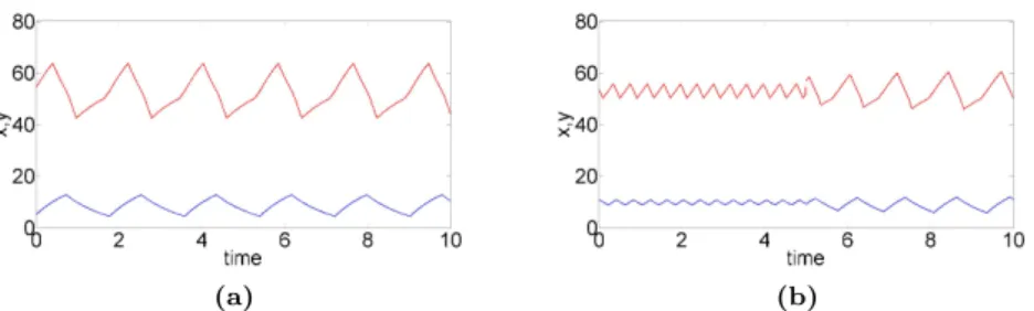
Although minimal, this 2-dimensional class of models can already account for a rich variety of dynamical phenomena. For appropriate parameter set-tings, this model displays different types of oscillatory behavior, from simple to more complex patterns, among which: damped oscillations towards a single equilibrium point (simulation not shown), a single oscillatory regime of sta-ble period and amplitude (Fig. 2a), birhythmicity with the coexistence of two stable oscillatory regime (Fig. 2b) separated by an unstable limit cycle (not shown).
(a) (b)
Fig. 2 Temporal simulations of x and y levels whose evolution is described
by Equations 1: (a) monorhythmic case with one large stable limit cycle; (b) birhythmic case with one large and one small stable limit cycles. A pulse of y is applied at t = 5 a.u. This pulse induces a shift from a small amplitude to a large amplitude oscillatory regime. Simulation of the level of x (resp. y) is shown in blue (resp. red). The initial conditions are x = 5.1,y = 54.3 for (a) and x = 10.6,y = 53.6 for (b). The parameter values are: θ1
y = 50, θy2 = 53, k2y = 15, dx = 1, dy = 1, k1y = 58, k1x = 20, θx= 10 and: k3y = 10 for (a); k3y= 5 for (b).
As precise quantitative information on kinetic parameters are generally miss-ing, predicting the conditions of emergence of oscillatory patterns from a qual-itative description of biological models, inferred from qualqual-itative information on the parameter values, is of particular interest. In the following, we derive theoretical results which set constraints on the oscillatory patterns which can emerge in a general class of 2-D PWA biological models according to topo-logical properties of its transition graph, a discrete qualitative description of this type of models. These structural principles will be derived using concavity and continuity properties of Poincar´e maps associated to cycles of the transi-tion graph (sectransi-tion 4). As a preliminary step, we first define the class of PWA biological models on which our analysis will be applied and the theoretical objects and tools which will be used to state our results (section 3).
3 Piecewise affine differential models
3.1 The general model
This paper focuses on the study of a general class of 2-dimensional piecewise affine (PWA) systems, with positive variables, (x, y)∈ ℜ+× ℜ+,ℜ+= [0,∞[:
dx dt = fx(x, y)− gx(x, y)· x dy dt = fy(x, y)− gy(x, y)· y (2)
where fi:ℜ+× ℜ+→ ℜ+and gi :ℜ+× ℜ+→ ℜ∗+ (i∈ {x, y}) are piecewise constant functions, representing the interactions between the various compo-nents of the system. The degradation of each component is assumed to be a linear process regulated by the components of the system.
The analysis of the system can be restricted to the phase space region: [0, Mx]× [0, My], with Mx= max{fgx(x,y)
x(x,y) : (x, y)≥ 0} and My= max{
fy(x,y)
gy(x,y) : (x, y)≥
0}, which defines a compact set that all trajectories enter and never leave (de Jong et al (2004)).
The variables x and y of the system are each associated with thresholds which set the switching values of the vector fields. We assume that x and y have nx and ny thresholds respectively:
0 < θ1 x< . . . < θxnx< Mx 0 < θ1 y< . . . < θ ny y < My with θ0
x= θ0y = 0. For convenience of notation, Mx and My will be renamed θnx+1
x and θ
ny+1
y respectively.
These thresholds partition the state space into (nx+ 1)· (ny+ 1) regular do-mains in which the vector fields are given by an affine function. These dodo-mains will be labelled using the following notation:
Dij : (i, j)∈ {1, 2, . . . , nx+ 1} × {1, 2, . . . , ny+ 1}, θxi−1< x < θ i
x and
θiy−1 < y < θyi
The segments and threshold intersections defining the borders of the regular domains are called switching domains. Such segments will be called switching segments and threshold intersections will be renamed switching points. In each regular domain Dij, the functions f
x, fy, gx and gy take constant values and the system can be rewritten as follows:
dx dt = k ij x − d ij xx dy dt = k ij y − d ij yy (3)
where fx= kijx, fy = kyij, gx= dijx and gy = dijy for (x, y)∈ D ij.
From Equations 3, we can define the so called focal points which are the points, ϕij, towards which the system tends monotically from each domain Dij(Glass and Pasternack (1978b)): ϕij = ( kij x dijx ,k ij y dijy ) .
The solutions of this system can be explicitly written: { x(t) =(x(0)− ϕijx ) · exp−dij xt+ϕij x y(t) =(y(0)− ϕijy ) · exp−dij yt+ϕij y (4) The equation of the trajectory in Dij can furthermore be derived by eliminat-ing time t. From Equations 4, we obtain:
y(t) =(y(0)− ϕijy)· ( x(t)− ϕij x x(0)− ϕijx )dijy dijx + ϕijy (5)
which defines the equation of the trajectory of the system in domain Dij. In the case of equal decay rates, dij
x = dijy = dij for all (i, j) and the trajectory in Dij is reduced to a straight line.
Throughout the paper, we will make the following assumptions:
Assumption 1. The focal points do not belong to the switching domains of
the phase space.
Therefore, if a regular domain Dijdoes not contain its focal point, the system will eventually escape this domain.
Assumption 2. Switching segments reached by a trajectory from a regular
domain are transparent walls i.e. the flow in these segments is well defined. Following Assumption 2, a trajectory reaching a switching segment can evolve into a contiguous regulatory domain, thus originating a transition between two regular domains. Stable solutions on switching segments (i.e called stable sliding modes in control theory (Casey et al (2005)) are thus excluded by this assumption. However, it may not be possible to continuously extend solutions reaching switching points. An approach originally proposed by Filippov (Fil-ippov (1988)) and more recently applied to PWA systems (Gouz´e and Sari (2002)) can then be used to define the solutions on switching points (see proof of Theorem 4 in Appendix A). An important consequence of Assumption 2 is the following lemma:
Lemma 1 For any initial condition, a solution of (2) which does not cross
switching points is unique.
The proof of this Lemma can be found in Appendix A. This property will be notably used in the analysis of the continuity of first return maps (see section 4.2).
Dij Dij Dij Dij Dij Dij Dij Dij
Fig. 3 Transition configurations arising from one vertex according to its focal
point position. The four configurations of the bottom are branching vertices
3.2 Transition graph and cycles 3.2.1 Transition graph
A discrete, qualitative description of the dynamics of a PWA system, initially proposed by Glass (Glass (1975a)), is called the transition graph: it is a di-rected graph whose vertices are the regular domains of the system and whose edges represent the possible transitions between these domains. The transition graph is obtained from the positions of the focal points.
Due to Assumption 2, each Dij will have either zero, one or two successors depending on the position of its focal point ϕij: Dij has no successor if ϕij belongs to Dij, and one successor (resp. two successors) if ϕij belongs to a contiguous regular domain which shares a switching segment (resp. a switch-ing point) boundary in common with Dij. The different types of escaping transition configurations from a vertex of the transition graph are summed up in Fig. 3. A vertex which has 2 successors is called branching vertex and the corresponding domain will be called branching domain. Each branching vertex gives rise to a curve (called separatrix ) emerging from the switching point defined by the intersection of the two switching segments crossed by the transitions leaving the branching vertex. The separatrix curve thus corre-sponds to the trajectory of the phase space which reaches this switching point. It delimits the branching domain into two subsets from which the system will either enter one successor domain or the other.
Combining two of these transitions gives rise to 3-vertex paths in the transition graph which will be of special interest in this work. These paths can be clas-sified in two categories: 3-vertex parallel paths, whose three regular domains are adjacent along two parallel switching segments, and 3-vertex perpendicu-lar paths, whose three reguperpendicu-lar domains are adjacent along two perpendicuperpendicu-lar switching segments. These two classes of paths will be called parallel motifs and perpendicular motifs respectively. The different types of parallel and
per-pendicular motifs are listed in Fig. 4 and 5. A trajectory passing through the domains composing a parallel (resp. perpendicular) motif will thus enter and escape the second domain through two parallel (resp. perpendicular) switching segments (Fig. 7). Finally, perpendicular motifs can be further classified into two subtypes: clockwise perpendicular motifs and counterclockwise perpendic-ular motifs (Fig. 5).
3.2.2 Transition cycles and n-cyclic attractors
We now introduce the following object. A transition cycle C of length n is defined as a periodic sequence of n vertices and n transitions in the transition graph:
Dr1s1 → Dr2s2 → . . . → Drnsn → Dr1s1
with (ri, si)∈ {1, . . . , nx+ 1} × {1, . . . , ny+ 1}, each vertex of the sequence being connected to its successor by a transition and no vertex appearing more than once in the sequence (see also Glass and Pasternack (1978b)). Note that the existence of a transition cycle does not imply the existence of a limit cycle for trajectories.
As we are in dimension two, we can moreover define the inside and the outside of a transition cycle C. The inside (resp. outside) of a transition cycle is the set of domains (regular and/or switching) which are located inside (resp. out-side) the transition cycle. Therefore, if a transition cycle contains a branching vertex, the transition from which the system can escape the cycle crosses a switching segment located either in the inside or the outside of the cycle. The former (resp. latter) type of transition will be called inside (resp. outside) branching transition of transition cycle C (see Fig. 10 for examples of inside and outside branching transitions). Transition cycles which do not contain one or the other type of branching transition will be considered when dealing with structural principles (section 4.3).
Transition cycles can be further classified in two broad categories according to the type of perpendicular motif composing the transition cycle: transition cycles which contain both clockwise and counterclockwise perpendicular mo-tifs (which will be called transition cycles with turn change) and transition cycles which contain only clockwise or only counterclockwise perpendicular motif (which will be called transition cycle with no turn change, see Fig. 10 for examples). The relevance of this classification will appear in section 4.2. An important class of cycles called cyclic attractors has been proposed by Glass and Pasternack (Glass and Pasternack (1978b)), which are cycles that do not contain branching vertices. We extend this notion of cyclic attractor to that of n-cyclic attractor. A n-cyclic attractor Cn is defined as the union of n transition cycles Ci of the transition graph:
Dij Di(j+1) Di(j-1) Dij Di(j+1) Di(j-1) Dij
D(i-1)j D(i+1)j D(i-1)j Dij
D(i+1)j
Fig. 4 Parallel motifs
Dij Di(j+1) D(i+1)j Dij Di(j+1) D(i+1)j Dij D(i-1)j Di(j-1) Dij D(i-1)j Di(j-1) Di(j-1) Dij D(i+1)j Di(j-1) Dij D(i+1)j Dij Di(j+1) D(i-1)j Dij Di(j+1) D(i-1)j
Fig. 5 Perpendicular motifs. Top: clockwise perpendicular motifs. Bottom:
counterclockwise perpendicular motifs.
Cn=∪C i
which does not contain vertices from which the system can escape the union of cycles. Thus, once a trajectory enters the union of the domains composing Cn, it will remain in these domains. Cyclic attractors defined by Glass and Pasternack are therefore 1-cyclic attractors.
In this paper, we will limit the scope of our work to transitioconnected n-cyclic attractors, which are n-n-cyclic attractors whose transition cycles share at least one transition in common (see Fig. 10 and 12 for examples). For sake of simplicity, transition-connected n-cyclic attractors will be renamed n-cyclic attractors.
3.3 Elementary maps and first return maps 3.3.1 Elementary maps
Since we assume there is no solution along switching segments (Assump-tion 2), a trajectory reaching the boundary of a regular domain will evolve into an adjacent domain by simply crossing the switching segments that sep-arate the two domains. Therefore, to each 3-vertex path Dk−1 → Dk → Dk+1 contained in the transition graph, we can define an elementary map Fk (Fk :ℜ+× ℜ+ → ℜ+× ℜ+) which maps the entering switching segment Dk−1
s to the escaping switching segment Dks which border Dk (see also Ed-wards (2000)). The image of a point of Dk−1
s by the map Fk is defined as the intersection of the trajectory starting from this point with Dks. Note that (in this 2-dimensional framework), each map Fk has a fixed coordinate at both the entering and escaping segments (see Fig.6).
In order to compute elementary maps, we define a scalar function fk (fk : ℜ+→ ℜ+) associated to the elementary map F
k by setting the direction and the origin of the axes supporting the entering and escaping switching segment, Dk−1
s and Dsk, where fkis computed. For each fk, two possible orientations can be chosen for the axis such that the origin coincides with either of the switch-ing point extremities, while the other extremity is assumed to be positive (see Fig.6). Once the origin and direction of the axis are set, the switching segment is said to be oriented. For convenience of notation, fk will also be called ele-mentary map of the 3-vertex path Dk−1 → Dk → Dk+1 and the axes where fk is computed will be called entering and escaping axes of fk.
Let Ik be the interval of definition of fk and lk the length of the entering switching segment of Fk. First, fk can be straightforwardly extended to the boundaries of Ik which are switching points. Then, if Dk is a not a branch-ing domain, the escapbranch-ing switchbranch-ing segment from Dk is unambiguous: all the points of Dk−1
s map Dsk. In this case, Ik = [0, lk]. If Dk is a branching domain, two cases can be distinguished according to the position of the separatrix curve which emerges in Dk: (1) the separatrix curve does not intersect Dk−1
s . In this case, either all the points of Dk−1
s map Dks and Ik = [0, lk], or none of the points of Dk−1
s map Dks and Ik = ∅ (Fig. 8, left). (2) The separatrix curve intersects Dk, splitting the entering switching segment of Dk in two segments. One of these segments will map Dk
s and the other not and Ik ⊂ [0, lk] (Fig. 8, right).
3.3.2 First return map of a transition cycle
We now assume that the transition graph of a PWA system contains a tran-sition cycle C of length n:
Fig. 6 Two choices of orientation for the axes of an elementary map of a
3-vertex parallel path D(i−1)j → Dij → D(i+1)j. Two possible orientations can be chosen for each axis such that the origin coincides with either of the switching point extremities, while the other extremity is assumed to be posi-tive. Red arrows represent the transition of the 3-vertex path. Blue ones are the entering and escaping axes where the elementary map of the 3-vertex path is computed.
with (ti, ui)∈ {1, 2, . . . , nx+ 1} × {1, 2, . . . , ny+ 1}.
Given a switching segment crossed by C, the associated first return map F (or Poincar´e map) (F :ℜ+× ℜ+ → ℜ+× ℜ+) is a mapping from this segment to itself, computed from two consecutive crossings of a trajectory of the system with this segment (Edwards (2000)). Let Di
sbe the switching segment crossed by the transition Dti−1ui−1 → Dtiui for i∈ {2, . . . , n} and D1
s the switching segment crossed by the transition from Dtnun to Dt1u1.
If Fiis the elementary map associated with the 3-vertex path: Dtnun→ Dt1u1 → Dt2u2 for i = 1, Dti−1ui−1 → Dtiui → Dti+1ui+1 for i ∈ {2, . . . , n − 1}
and Dtn−1un−1 → Dtnun → Dt1u1 for i = n, the first return map F of the transition cycle C from and to the switching segment D1s is the composite of the elementary maps Fi for i∈ {1, 2, . . . , n}:
F = Fn◦ Fn−1◦ . . . F1
The domain of definition of F is called the returning cone of F (Edwards (2000)).
As for an elementary map, in order to compute the first return map of C, we can define a scalar function f (f : ℜ+ → ℜ+) associated with the first return map F by setting the direction and the origin of the axis supporting the switching segment D1
s where f is computed. The origin of the axis is set in the same manner as the origin of the axes of elementary maps (see previous section). f will also be called the first return map from and to Ds1of transition cycle C.
Let the escaping axis of Dtiui and the entering axis of Dti+1ui+1 have the
same orientation. Let fi be the elementary map associated with the 3-vertex path: Dtnun → Dt1u1 → Dt2u2 for i = 1, Dti−1ui−1 → Dtiui → Dti+1ui+1 for
i∈ {2, . . . , n − 1} and Dtn−1un−1 → Dtnun → Dt1u1 for i = n. f is then the composite of the elementary maps fi for i∈ {1, 2, . . . , n}:
f = fn◦ fn−1◦ . . . f1
3.3.3 First return map of a n-cyclic attractor
We assume that the transition graph contains an n-cyclic attractor Cn com-posed of the n transition cycles Ci for i∈ {1, 2, . . . n}. Let Ds be an oriented switching segment crossed by a transition common to all Ci and let l be the length of the segment Ds.
Let Dbv1, Dbv2, . . . , Dbvm be the branching vertices of Cn. Each branching
vertex Dbvi gives rise to a separatrix curve. Let x1
s< x2s < . . . < xps (p6 m) be the coordinates of the last intersection (if it exists) between the trajecto-ries lying in the separatrix curves and Ds before these trajectories reach a switching point. The xispartition Dsinto (p + 1) segments Ii:
I1= [ 0, x1 s [ , Ii= ] xi−1 s , xis [ for 2≤ i ≤ p and Ip+1 = ]xps, l].
Each trajectory starting from a point whose coordinate belongs to Ii will thus follow a distinct transition cycle Cui in the transition graph before a first
re-turn in Ds. Note that all the cycles composing Cnare not necessarily followed by a trajectory starting from Ds.
Ii then defines the interval of definition of the first return map bfi associated to Cui from and to the oriented switching segment Ds. We can then define a
map bf on the union of intervals I =∪Ii as follows:
for i∈ {1, 2, . . . , n}: bf (x) = bfi(x) for x∈ Ii b
f will be called n-cycle first return map of the n-cyclic attractor Cn from and to the oriented switching segment Ds.
In the following, we will limit our work to the case n ≤ 2. In the case of a 1-cyclic attractor (which corresponds to a cyclic attractor as defined by Glass and Pasternack (1978b)), there is no branching vertex and I = [0, l]. In the case of a 2-cyclic attractor, we state the following lemmas (see Appendix A for the derivation of the proofs). Let C2be a 2-cyclic attractor and DC2the union of the domains composing C2.
There is therefore a single separatrix curve in the domains composing a 2-cyclic attractor which emerges from the unique branching vertex. There is also a unique vertex where the transition cycles composing C2 merge. The properties of the subgraph composed of the two distinct pathways linking the branching and the merging vertices will be of special interest when dealing with the continuity of the first return map of 2-cyclic attractors (section 4.2).
Lemma 3 Two different trajectories cannot intersect in DC2. This Lemma will be notably used in the proof of Theorem 4.
4 Results
4.1 Monotonicity and concavity properties of an elementary map
In this section, the monotonicity and the concavity properties of the elemen-tary maps fk of the different types of parallel and perpendicular motif (listed in Fig. 4 and 5) are studied. The proofs of the following statements can be found in Appendix A.
We first state a lemma which will be used to derive the monotonicity and concavity properties of elementary maps established in Propositions 1 and 2.
Lemma 4 Let fk be an elementary map. Assume fk is monotone and of con-stant concavity. Then, changing the orientation of the entering axis of fk changes the monotonicity but does not change the concavity of fk. Chang-ing the orientation of the escapChang-ing axis of fk changes the monotonicity and concavity of fk.
Proposition 1 Let fk be the elementary map of a parallel motif. Then fk is an affine function. If the entering and escaping axes of fk have the same ori-entation, fk is an increasing function. Otherwise, fk is a decreasing function.
Proposition 2 Let fk be the elementary map of a perpendicular motif and Sk the switching point at the intersection of the entering and escaping segment of fk.
(1) If the entering and escaping axes of fk are both oriented either towards or away from Sk, fk is increasing. Otherwise fk is decreasing.
(2) If the origin of the escaping axis is Sk, fk is strictly concave. Otherwise, it is strictly convex.
Note that elementary maps are continuous functions (see analytical expression of fkin the proofs of Propositions 1 and 2). These results on the monotonicity and concavity of elementary maps will be used in the next section to derive monotonicity and concavity properties of first return maps.
Fig. 7 An example of oriented perpendicular motif (left) and parallel motif
(right) with entering axis [0, z1) and escaping axis [0, z2). The red arrows are the transitions compos ing each motif. The elementary map associated to the perpendicular (resp. parallel) motif is increasing and strictly concave (resp. affine). A trajectory of the system from the entering to the escaping axis is indicated in blue arrow
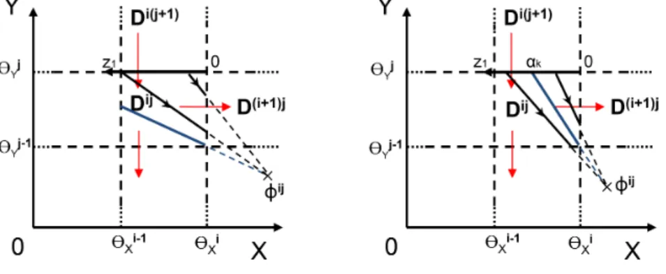
Fig. 8 Two cases for separatrix curve position. (left) The separatrix curve
does not intersect the entering segment{θi−1
x < x < θxi, y = θyi }
of the 3-vertex path Di(j+1) → Dij → D(i+1)j. The domain of definition of the associated el-ementary map is the whole entering segment. (right) The separatrix curve intersects the entering segment{θi−1
x < x < θxi, y = θiy }
of the 3-vertex path
Di(j+1) → Dij → D(i+1)j at z1= αk. The domain of definition of the
associ-ated elementary map is [0, αk[. The separatrix curves are drawn in blue and trajectories in black
4.2 Monotonicity, concavity and continuity properties of first return maps We now state general properties of first return maps concerning their mono-tonicity, concavity and continuity. Theorems 1, 2 and 3 concern the properties of monotonicity and concavity of the first return map of a transition cycle. Theorem 4 deals with continuity properties of 2-cycle first return maps. These properties will be used in the next section to derive structural principles linking the topology of the cycles in the transition graph to the number and stability of limit cycles. The proofs of the theorems can be found in Appendix A. For Theorems 1, 2 and 3, we assume that the transition graph contains a transition cycle C.
Theorem 1 (Monotonicity) The first return map of a transition cycle C is
an increasing and continuous function.
Theorem 2 (Concavity for equal decay rates) Assume the decay rates
are equal in each domain Dij, i.e. dijx = dijy for (i, j) ∈ {1, 2, . . . , nx+ 1} × {1, 2, . . . , ny+ 1}). Then the first return map of C has a constant and strict concavity.
Theorem 3 (Concavity for transition cycles with no turn change)
Assume C is a transition cycle with no turn change. If the axis of definition of the first return map f of C is oriented towards the outside of C, f is strictly concave. Otherwise, f is strictly convex.
We now assume that the transition graph contains a 2-cyclic attractor C2, composed of two transition cycles C1and C2. According to Lemma 2, C2 con-tains a single branching and a single merging vertex. Let DS and DT be the branching and merging vertices respectively of C2 and SG
S→T the subgraph composed of the two distinct pathways linking DS to DT.
Let S be the switching point from which emerges the separatrix curve in DS (see Fig. 9). Let DC be an oriented switching segment crossed by a common transition of C1and C2. Assume that the separatrix curve emerging from the branching vertex of C2 intersects D
C and let α be the coordinate of the last intersection between DC and the trajectory lying in the separatrix curve be-fore it reaches S. Let bf be the 2-cycle first return map of C2calculated on the oriented segment DC:
{ bf (x) = bf1(x) for x∈ [0, α[ b
f (x) = bf2(x) for x∈ ]α, l]
(6)
where bf1and bf2are the first return maps of C1and C2respectively calculated on DC, and l the length of DC. The following theorem states the topological conditions on a 2-cyclic attractor for its 2-cycle first return map to be extended to a continuous function.
Theorem 4 (Continuity of a 2-cycle first return map) bf can be extended to a continuous function in [0, l] iff SGS→T is composed of only 4 vertices.
Y
X
0
ϴY ϴX SD
1(D
S)
D
3D
2D
4(D
T)
Y
X
0
ϴY ϴX SD
1(D
S)
D
3D
2D
4D
TFig. 9 Two examples of transition graph containing a 2-cyclic attractor. (left)
SGS→T is a 4-node subgraph. (right) SGS→T contains more than 4 nodes (here 6 nodes). The red arrows are the transitions composing the subgraph SGS→T. The black arrows are the transitions connecting SGS→T to the rest of the transition graph (not shown). The trajectory lying in the separatrix reaches the switching point S and either does not split (left) or split into two distinct trajectories (right). In both cases, D1corresponds to a branching vertex (ϕ1
x−θx> 0 and ϕ1y−θy < 0). In the left case, D2and D3communicate with D4(ϕ2x−θx> 0, ϕ3y−θy < 0) leading to a 4-node SGS→T, whereas in the right case D4 does not communicate with D2 (ϕ2x− θx< 0 and ϕ4x− θx > 0) leading to a SGS→T composed of more than 4 nodes. According to Theorem 4, the left case gives a continuous first return map, which is discontinuous in the right case.
4.3 Structural principles
From the previous theorems, we can derive structural principles, i.e. properties which emerge from the structure of the transition graph, on the number and stability of the limit cycles (Lu and Edwards (2010)). These structural princi-ples are limited to the cases where either C has no turn change or the decay rates are equal, which are cases for which information about the concavity of
the first return map have been obtained (see Theorems 2 and 3). The analysis of the number of limit cycles (i.e. fixed points of the first return maps) is only considered in the generic case, when the intersections between the first return map and the identity are transverse (see Fig.14). The first structural principle is a general principle which states the maximum number of stable and unstable limit cycles a system can have in the domains of the phase space crossed by C. The second and third structural principles state constraints on the number and stability of limit cycles for specific topological properties of the transition graph. Finally, the last theorem concerns the number of unstable limit cycles for a 2-cyclic attractor when specific topological conditions on the structure of the transition graph are fulfilled (see Theorem 4). The proofs of the following statements can be found in Appendix A.
For the first three structural principles (Theorems 5, 6 and 7), we assume that the transition graph contains a transition cycle C and call DC the union of the domains composing C. Let f be a first return map of C, I the interval of definition of f and l the length of the switching segment where f is calculated.
Theorem 5 (First structural principle) Assume that either (1) C is a
transition cycle with no turn change or (2) the decay rates are equal. Then there are at most two limit cycles in DC. If there are two limit cycles in DC, one is stable and the other is unstable.
The following lemma will be used to prove the next two structural principles.
Lemma 5 We assume that the axis where f is calculated is oriented towards
the outside of C.
(a) Assume C contains no inside branching transition. Then if I̸= ∅, 0 ∈ I. (b) Assume C contains no outside branching transition. Then if I̸= ∅, l ∈ I.
Theorem 6 (Second structural principle) Assume that C is a transition
cycle with no turn change. If C contains no inside branching transition, the system does not admit an unstable limit cycle in DC but either (1) has no limit cycle or (2) has one single stable limit cycle in DC.
Theorem 7 (Third structural principle) Assume that either (1) C has
no turn change or (2) the decay rates are equal. If C contains no outside branching transition and if the system admits an unstable limit cycle in DC then it admits a single stable limit cycle in DC.
Note that information about the concavity of the first return map is required for Theorem 6 whereas only a constant concavity is needed for Theorem 5 and 7, which explains why Theorem 6 only applies to the case where C has no turn change and not the case where the decay rates are equal.
For the last structural principle, we assume that the transition graph con-tains a 2-cyclic attractor C2, composed of transition cycles C1 and C2. Let DC be a switching segment crossed by a common transition to C1 and C2,
and DC2 the union of the domains composing C2. Let SGS→T be the sub-graph composed of the two distinct pathways linking the branching vertex of C2to the vertex where C1and C2 merge.
Theorem 8 (Fourth structural principle) Assume that either (1) C1and C2 have no turn change or (2) the decay rates are equal. Assume also that SGS→T is composed of 4 vertices. If the system admits two stable limit cycles in DC2
, there exists a unique unstable limit cycle in DC2
which delimits the basin of attraction of the two stables limit cycles.
5 Applications
Two applications of the previous theoretical results will be described in this section. Both applications represent PWA models of biological oscillators whose transition graph is composed of a 2-cyclic attractor. All the possible dynamical configurations in terms of the number and the stability of the limit cycles are derived using the structural principles stated in the previous section. In the first application, which corresponds to a case where the 2-cycle first return map is continuous, the oscillatory behavior of the case study presented in section 2 is revisited in the light of our theoretical results. The second application con-cerns a more complex biological oscillator whose transition graph reproduces the one of a reduced version of the p53-Mdm2 network model (Abou-Jaoud´e et al (2009); Abou-Jaoud´e et al (2011)) and for which the 2-cycle first return map is discontinuous.
5.1 A continuous first return map
We consider the class of 2D-piecewise affine differential models introduced in section 2 which represents a minimal model for biological oscillators (see Equa-tions 1). The interaction graph, shown in Fig. 1b, is composed of one 2-element negative feedback loop and two 1-element positive feedback loops. The step functions partition the phase space into 6 domains delimited by threshold θx along x, and thresholds θ1
y and θ2y along y. The parameter value sets have been chosen such that transition graph is the 2-cyclic attractor indicated in Fig. 10. This attractor is composed of two embedded transition cycles: one 4-elements cycle D22 → D12→ D13→ D23 → D22 (transition cycle C
1) and one 6-elements cycle D11→ D12→ D13→ D23→ D22→ D21→ D11 (transi-tion cycle C2). The branching vertex is D22 and the vertex where both cycles merge is D12.
Let DC1 (resp. DC2) be the union of the domains composing C
1 (resp. C2). C1 and C2 have no turn change. Moreover, cycle C1 has no inside branch-ing transition. Therefore, accordbranch-ing to the second structural principle, the system admits no unstable limit cycle and at most one stable limit cycle in DC1. Cycle C
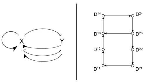
Fig. 10 Transition graph for the continuous case. The transition graph is
composed of two transition cycles which form a 2-cyclic attractor: cycle D22 → D12 → D13 → D23 → D22 (transition cycle C
1) and cycle D11 → D12 → D13 → D23 → D22 → D21 → D11 (transition cycle C
2). C1 contains one outside branching transition (D22 → D21) whereas C
2 contains one inside branching transition (D22 → D12). C
1and C2 have no turn change
structural principle, if the system admits an unstable limit cycle in DC2, it admits a stable limit cycle in DC2. At most two stable limit cycles and one unstable limit cycle is therefore possible in the union of domains DC1and DC2. Finally, the subgraph composed of the two paths linking the branching vertex to the vertex where both cycles merge contains 4 vertices: D22, D21, D11and D12. Therefore, according to the fourth structural principle, if the system ad-mits two stable limit cycles, there exists a unique unstable limit cycle which delimits the basin of attraction of the two stable limit cycles.
Thus, the dynamical configurations of this system in terms of the number and the stability of the limit cycles are limited to at most the following five cases:
(a) one large stable limit cycle located in DC2; (b) one small stable limit cycle located in DC1;
(c) one large stable limit cycle and one unstable limit cycle both located in DC2;
(d) one small stable limit cycle located in DC1, and one large stable limit cycle and one unstable limit cycle located DC2. The unstable limit cycle delimits the basins of attraction of the stable limit cycles;
We could actually find parameter value sets corresponding to each of the five dynamical configurations stated above. Fig. 11 shows numerical simulations in the phase space corresponding to cases (a),(b),(c) and (d) (cases for which there is at least one limit cycle). The parameter sets for the two oscillatory patterns displayed by the case study in Fig. 2 correspond to cases (a) and (d). The corresponding 2-cycle return maps are described in Appendix B.
Fig. 11 Numerical simulations for the continuous case corresponding to the
possible dynamical configurations derived from the structural principles: case with one large stable limit cycle (top left); one small stable limit cycle (top right); one large stable limit cycle and one unstable limit cycle (bottom left); one large and one small stable limit cycles and one unstable limit cycle (bottom right). The stable (resp. unstable) limit cycles are drawn in blue (resp. in red). The parameter values for the top left and bottom right figures are indicated in the legend of Fig. 2. The parameter values for the others figures are: θ1
y= 50, θ2
y = 53, k2y= 15, dx= 1, dy = 1 and: k1y = 58, k1x = 20, k3y = 5, θx= 20 (top right); k1y = 54, k1x = 30, k3y = 0, θx = 10 (bottom left). The system admits one stable equilibrium point at (θx, θ2y) and no limit cycle for k1y= 58, k1x= 20, k3y= 0, θx= 10 (simulation not shown).
Fig. 12 Discontinuous case: graph of interactions (left) and transition graph
(right). The transition graph is composed of two transition cycles which form a 2-cyclic attractor: cycle D23 → D13 → D14→ D24→ D23(transition cycle C1) and cycle D11 → D12 → D13 → D14 → D24 → D23 → D22 → D21 → D11(transition cycle C2). C1 contains one outside branching transition (D23 → D22) whereas C
2 contains one inside branching transition (D23→ D13)
5.2 A discontinuous first return map
We now consider the following class of 2D-piecewise affine differential models: dx dt = [ k1x+ k2x· s+(y, θy1) ] · s−(y, θ2 y)· s +(x, θ x) + s+(y, θ3y))·[k3x+ k4x· s+(x, θx) ] − dx· x dy dt = k1y· s −(x, θ x)− dy· y (7)
where s+ and s− are step functions as previously defined in section 2. The interaction graph, shown in Fig. 12, is composed of two 2-element neg-ative feedback loops and two positive feedback loops (one 1-element and one 2-element). The step functions partition the phase space into 8 domains de-limited by threshold θxalong x, and thresholds θ1y, θ2yand θ3y along y. The pa-rameter value sets have been chosen such that transition graph is the 2-cyclic attractor indicated in Fig. 12. This graph reproduces the transition graph of a reduced version of the p53-Mdm2 network model (Abou-Jaoud´e et al (2009)) analyzed in Abou-Jaoud´e et al (2011).
The transition graph is composed of two embedded transition cycles: one 4-element cycle D23→ D13→ D14→ D24→ D23(transition cycle C1) and one
8-element cycle D11 → D12 → D13 → D14 → D24 → D23 → D22 → D21 → D11(transition cycle C2). The branching vertex is D23 and the vertex where both cycles merge is D13.
Let DC1 (resp. DC2) be the union of the domains composing C
1 (resp. C2). As for the continuous case, both cycles have no turn change. Cycle C1 has no inside branching transition while cycle C2has no outside branching transition. The second and third structural principles can thus both be applied for C1 and C2respectively.
However, the subgraph composed of the two paths linking the branching ver-tex to the verver-tex where both cycles merge contains now 6 vertices: D23, D22, D21, D11, D12 and D13. Therefore, the fourth structural principle cannot be applied. One supplementary dynamical configurations in terms of the number and the stability of the limit cycles could thus arise in addition to the five dynamical configurations which appear in the previous example:
(f) two stable limit cycles, one located in DC1, the other in DC2.
In this additional configuration, the two stable limit cycles are not separated by an unstable limit cycle but by the separatrix curve emerging in the branch-ing vertex D23 (Fig. 12) from the threshold intersection (θ
x, θy2).
We could actually find parameter value sets corresponding to each of the six possible dynamical configurations. Fig. 13 shows numerical simulations corre-sponding to cases (a),(b),(c), (d) and (f) (cases for which there is at least one limit cycle). The corresponding 2-cycle return maps are listed in Appendix B. Fig.10B of Abou-Jaoud´e et al (2011) gives another numerical example of the case where the system has two stable limit cycles and no unstable limit cycle (case (f)).
6 Discussion
In this work, we derived structural principles linking the topology of the tran-sition graph of a class of 2-dimensional piecewise affine biological models to the number and stability of limit cycles. To do so, we analyzed the continu-ity, monotonicity and concavity properties of Poincar´e maps associated to the transition cycles of the transition graph. In the case of nonequal decay rates, structural principles linking the topology of a transition cycle to the dynam-ics of the system in terms of number and stability of limit cycles have been determined when the transition graph contains no turn change. For 2-cyclic attractors in the transition graph, structural principles have been derived on the number of unstable limit cycles from the continuity of the first return map associated to the attractor. The results of our work have then been applied to two biological cases whose transition graph are 2-cyclic attractors: a case for which the first return map is continuous, a case for which the first return map is discontinuous.
Fig. 13 Numerical simulations for the discontinuous case corresponding to
the possible dynamical configurations derived from the structural principles: case with one large stable limit cycle (top left); one small stable limit cycle (top right); one large stable limit cycle and one unstable limit cycle (middle left); one small and one large stable limit cycle and one unstable limit cycle (middle right); one small and one large stable limit cycles (bottom left). Stable (resp. unstable) limit cycles are drawn in blue (resp. in red). The parameter values are: θ1
y = 10.1, θ2y = 10.2, θ3y = 10.5, k1x = 29, k2x = 2, k3x = 35, k1y = 12.5, dx = 1, dy = 1 and:θx= 5, k4x = 4 (top left), θx = 50, k4x = 4 (top right), θx = 8, k4x = 0 (middle left), θx = 30, k4x = 4 (middle right), θx= 20, k4x= 4 (bottom left). The system admits no limit cycle (one stable equilibrium point at (θx, θy3)) for θx= 30, k4x= 0 (simulation not shown)
The mathematical tractability of the class of PWA biological models analyzed in our work allows to derive the stated structural conditions on the number and stability of limit cycles. Such results on the number of limit cycles cannot be derived in ODE systems. For planar ODE systems, Poincar´e-Bendixson the-orem gives mathematical conditions for the existence of limit cycles but there is no general theoretical results on the number of limit cycles. More specific
results concern the number or stability of limit cycles, but for more specific systems (Lienard systems, polynomial systems...) and may be rather complex (see (Perko, 1991, p. 234) for references). To investigate whether the struc-tural results obtained for the class of PWA models considered in our work are conserved in the continuous framework, we translated the PWA system of the discontinuous case (section 5.2) into an ODE model by replacing step functions with Hill functions. Interestingly, for appropriate parameter values, a first nu-merical analysis of this model suggests that the discontinuity observed in the PWA model has some counterpart in the continuous framework (Appendix C). The extension of our results to higher dimension PWA systems seems to be difficult to achieve since the conclusions stated in our work strongly rely on the topological constraint imposed by the 2-dimensional space. However, several developments of this work can be considered. First, for unequal decay rates, the structural principles derived here are restricted to the case where transition cycles have no turn change. Under this condition, properties on the concavity of first return maps associated with transition cycles can be derived. These properties are then used to determine the structural principles on the number and the stability of limit cycles in the domain of the phase plane covered by a transition cycle of this type. An extension of the concavity results when tran-sition cycles contain a turn change still has to be investigated. First results on this issue show that we can conclude on the monotonicity and concavity properties for some specific topological structures of the transition graph (re-sults not shown). Secondly, this work focused on the continuity properties of 2-cycle first return maps. An extension of these results to n-cycle first return maps associated with n-cyclic attractors for n≥ 3 can also be investigated. Finally, applications of these structural principles contribute to gain intuition on the dynamical behavior of biological networks and provide guidance on pa-rameters or experimental conditions that generate a given behavior.
7 Acknowledgements
We would like to thank Denis Thieffry for critical reading of the manuscript, and also on of the reviewers for his careful reading and many useful sug-gestions. W. Abou-Jaoud´e was supported in part by the LabEx MemoLife (www.memolife.biologie.ens.fr). M. Chaves and J.L. Gouz´e were supported in part by the projects GeMCo (ANR 2010 BLANC020101), ColAge (Inria-Inserm Large Scale Initiative Action), RESET (Investissements dAvenir, Bioin-formatique), and also by the LABEX SIGNALIFE (ANR-11-LABX-0028-01).
A Proofs
Lemma 1.
Proof In regular domains, the evolution of the system is described by continuous affine
differential equations. Therefore, for a given an initial condition, the solution of system (2) in each regulatory domain is unique.
Moreover, the switching segments are all transparent. Thus, when a trajectory reaches a switching segment, it can be continued into its contiguous regular domain.
Therefore, a solution of the system which does not cross a switching point is unique, which ends the proof.
Lemma 2.
Proof The proof of this lemma can be straightforwardly derived from the definition of a
2-cyclic attractor, which is the union of two transition cycles sharing at least a transition in common and which does not contain vertices from which the system can escape the 2-cyclic attractor.
Lemma 3.
Proof First, two different trajectories cannot intersect in a point which is not a switching
point according to Lemma 1. Then assume that they intersect on a switching point. The two trajectories would then pass through two different domains before reaching the switching
point. This implies that C2would contain more than 1 branching vertex which is forbidden
by Lemma 2.
Lemma 4.
Proof let l be the length of the entering switching segment of fk. Changing the direction of the entering axis is equivalent to transform z→ l − z. Moreover:
d [fk(l− z)] dz =− dfk dz(l− z) and d2[fk(l− z)] dz2 = d2fk dz2 (l− z)
Thus changing the direction of the entering axis changes the monotonicity but does not change the concavity of fk.
Changing the direction of the escaping axis is equivalent to transform fk(z)→ l − fk(z).
Moreover: d [l− fk(z)] dz =− dfk dz(z) and d2[l− fk(z)] dz2 =− d2fk dz2 (z)
Therefore, changing the direction of the escaping axis changes the monotonicity and con-cavity of fkwhich ends the proof.
Proposition 1. Proof let f1
k, fk2, fk3 and fk4 be the elementary maps of the four parallel motifs (listed in
Fig. 4) : Di(j−1)→ Dij→ Di(j+1), Di(j+1)→ Dij→ Di(j−1), D(i+1)j→ Dij→ D(i−1)j
and D(i−1)j → Dij→ D(i+1)j respectively, with the entering and escaping axes oriented
along axis [0,x), for f1
k and fk2, and [0,y), for fk3and fk4.
The analytical expression of f1
k and fk2are derived by replacing in Equation 5:
- (x(0), y(0)) = (z + θix−1, θiy−1) and (x(t), y(t)) = (fk(z) + θix−1, θiy) for fk1;
fk1(z) = ( z + θix−1− ϕijx ) ·( θiy−ϕijy θi−1y −ϕijy )dijx dijy + ϕij x − θix−1with ϕijy > θiy. f2 k(z) = ( z + θxi−1− ϕijx ) · ( θi−1y −ϕij y θi y−ϕ ij y )dijx dijy + ϕij x − θix−1with ϕijy < θyi−1. Let a = θxi−1− ϕijx, b = θi y−ϕijy θi−1y −ϕijy and c =dijx dijy . Then we have: f1 k(z) = b c· (z + a) − a fk2(z) = (1/b)c· (z + a) − a Therefore, f1
kand fk2are affine functions. As b > 0, fk1and fk2are increasing affine functions.
The analytical expression of f3
kand f
4
kare derived by exchanging x and y in the expression
of f1 kand f 2 k respectively. Thus, f 3 k and f 4
k are also increasing affine functions.
Finally, according to Lemma 4, changing the orientation of either the entering or escap-ing axis changes the monotonicity of an elementary map, which ends the proof.
Proposition 2. Proof Let f1
k, fk2, fk3, fk4, fk5, fk6, fk7, fk8 be the elementary maps of the 8 perpendicular
mo-tifs (listed in Fig. 5): D(i+1)j → Dij → Di(j+1), D(i−1)j → Dij → Di(j−1), Di(j+1)→ Dij → D(i−1)j, Di(j−1) → Dij→ D(i+1)j, Di(j+1)→ Dij → D(i+1)j, Di(j−1) → Dij → D(i−1)j, D(i+1)j → Dij → Di(j−1) and D(i−1)j → Dij → Di(j+1)respectively, and Si
kthe switching point at the intersection of the entering and escaping segment of fki. We
assume that the origin of the entering and escaping axes of fi kis Ski.
The analytical expression of f1
k, f 2 k, f 3 k and f 4
k are derived by replacing in Equation 5:
- (x(0), y(0)) = (θi
x, θiy− z) and (x(t), y(t)) = (θxi− fk(z), θiy) for fk1;
- (x(0), y(0)) = (θxi−1, z + θiy−1) and (x(t), y(t)) = (fk(z) + θxi−1, θiy−1) for fk2;
- (x(0), y(0)) = (θix−1+ z, θiy) and (x(t), y(t)) = (θ i−1
x , θyi− fk(z)) for fk3;
- (x(0), y(0)) = (θi
x− z, θiy−1) and (x(t), y(t)) = (θix, θyi−1+ fk(z)) for fk4:
f1 k(z) =− ( θyi−ϕijy θi y−ϕijy−z )dijx dijy ·(θi x− ϕ ij x ) + θi x− ϕ ij x with ϕijx < θxi and ϕ ij y > θiy f2 k(z) =− ( θi−1y −ϕijy θi−1y −ϕijy+z )dijx dijy ·(ϕij x − θxi−1 ) + ϕijx − θxi−1with ϕijx > θix−1and ϕijy < θyi−1 f3 k(z) =− ( θi−1x −ϕij x θi−1x −ϕijx+z )dijy dijx ·(θi y− ϕ ij y ) + θi y− ϕ ij y with ϕijy < θiyand ϕ ij x < θix−1 f4 k(z) =− ( θix−ϕij x θi x−ϕijx−z )dijy dijx ·(ϕij y − θiy−1 ) + ϕijy − θiy−1with ϕijy > θyi−1and ϕijx > θix fi
k(z) for i ={1, 2, 3, 4} are thus of the form: −( b
b+z
)c a + a