Analysis of boundary representation model rectification

Analysis of Boundary Representation Model Rectification

Guoling Shen

B.S. in Naval Architecture and Marine Engineering (1988) Huazhong University of Science and Technology, China M.S. in Naval Architecture and Marine Engineering (1997)

M.S. in Mechanical Engineering (1997) Massachusetts Institute of Technology

Submitted to the Department of Ocean Engineering in partial fulfillment of the requirements for the degree of

Doctor of Philosophy at the

MASSACHUSETTS INSTITUTE OF TECHNOLOGY June 2000

@

A u th o r ... ... ... Department of Ocean Engineering

February 9, 2000

C ertified b y ...

Nicholas M. Patrikalakis Kawasaki Professor of Engineering Thesis Supervisor Accepted by .... MASSACHUSETTS INSTITUTE OF TECHNOLOGY

NOV 2 9 2000

Analysis of Boundary Representation Model Rectification

by

Guoling Shen

Submitted to the Department of Ocean Engineering , on February 9, 2000, in partial fulfillment of the

requirements for the degree of Doctor of Philosophy

Abstract

One major disadvantage of boundary representation (B-rep) is its inability to guar-antee model validity. This thesis addresses issues on model validity verification and defect rectification. We first study validity of ideal B-rep models. In particular, we derive a complete set of conditions for validity of representational nodes of a general B-rep data structure and prove their sufficiency. A representational node defines a valid topological boundary entity if it satisfies the corresponding conditions and all its lower level nodes are valid. We then analyze the model rectification problem, and propose a rectify-by-reconstruction approach which searches for the global optimal solution. Such a reconstruction method rebuilds a valid boundary which is topologi-cally equivalent to a given B-rep model and has the minimum geometric change. It is also shown that the boundary reconstruction problem is NP-hard. Based on this, a boundary reconstruction methodology is proposed which aims to build a valid bound-ary in the neighborhood of the original model and duplicate its topological structure as much as possible. Finally, we use interval model representation in boundary re-construction. An interval model is defined as a collection of boxes, and is regarded as an approximation of the intended exact model. We also define the concept of approx-imate equality relation between an interval model and its intended exact model, and derive sufficient conditions for such approximate equality. Such a relation imposes constraints on geometric and topological properties of interval models. Techniques needed in interval model construction are also developed. An example illustrates some of the issues discussed in this thesis.

Thesis Supervisor: Nicholas M. Patrikalakis Title: Kawasaki Professor of Engineering

Acknowledgments

Funding for this work was obtained in part from NSF grant DMI-9215411, ONR grant N00014-96-1-0857 and from the Kawasaki chair endowment at MIT.

I thank my advisor, Prof. N. M. Patrikalakis, for guiding me through the labyrinth of scientific research, and Prof. T. Sakkalis, whose help greatly improved the mathe-matical rigor of this work. Most of the ideas presented in this thesis were developed from our (exhausting but very productive) discussions in Athens last spring.

I would also like to thank other members of my thesis committee, Prof. D. C. Gossard, Prof. J. Peraire, and Dr. X. Ye, for their constructive comments. Dr. X. Ye also provided the example used in this thesis.

Thanks also go to Prof. A. Clement, Prof. T. J. Peters, Prof. A. Russell and Prof. F.-E. Wolter for useful discussions and comments, to Dr. W. Cho and Mr. G. Yu for their assistance in the early phases of the CAD model rectification project, and to Mr. F. Baker for maintaining a reliable hardware environment.

I also thank all Design Laboratory members, former and present, for making the laboratory a pleasant working place.

I want to take this chance to thank all my friends, especially Liangwu, Qinghua, Yining, Dan, Yujing, Wenjie, Xiaopeng, and Pimjai, for always being there for me.

I thank my family for their love and support. Especially, I thank my wife, Zheng, for her love, and for sharing her dream with me.

Contents

1.1 _{M otivation and Objectives . . . .} 1.2 CAD M odel Defects. . . . . 1.3 Thesis Organization. . . . . 2 Literature Review

2.1 Manifold B-Rep Model Validity 2.2 CAD Model Rectification...

2.2.1 Polyhedral models . . . . 2.2.2 Surface models . . . . 2.3 Robust Geometric Representation

3 Representational Validity of Boundary Representation Models 3.1 _{Mathematical Preliminaries . . . .} 3.2 _{Solids and their Boundaries . . . .} 3.3 Representational Validity Conditions . . . . 3.3.1 D ata structure _{. . . .} 2 3 4 7 9 9 11 14 16 . . . . 16 . . . . 18 . . . . 19 . . . . 2 1 . . . . 23 26 26 29 35 35

3.3.2 3.3.3

Sufficient conditions for node validity . . . . Proof of validity . . . .

4 Analysis of Manifold Boundary Representation Model Rectification 4.1 Problem Statem ent . . . . 4.2 Problem Com plexity . . . . 4.2.1 Face reconstruction problem . . . . 4.2.2 Boundary reconstruction problem . . . .

5 Topological and Geometric Properties of Interval Solid Models 5.1 Introduction . . . . 5.2

5.3

Covering Manifolds with Boxes . . . . Construction of Interval Solids . . . .

6 Manifold Boundary Representation Model Rectification 6.1 Introduction . . . .

6.2 Surface Intersection and Box Construction 6.2.1 Surface intersection . . . . 6.2.2 Control of box size . . . . 6.2.3 Structure of intersection boxes . . . 6.2.4 Data reduction . . . .

6.3 Model Reconstruction Methodology . . . .

6.3.1 Overview . . . . 6.3.2 Intersection-induced graph . . . . . 6.3.3 Face reconstruction . . . . 6.3.4 Shell reconstruction . . . . 6.4 Exam ple . . . .

7 Conclusions and Recommendations

7.1 Conclusions . . . . 7.2 Recommendations . . . . 36 38 41 41 45 45 57 61 61 62 68 77 . . . . 7 7 . . . . 78 . . . . 78 . . . . 79 . . . . 8 1 . . . . 8 5 . . . . 8 7 . . . . 8 7 . . . . 89 . . . . 89 . . . . 94 . . . . 96 100 100 101

A Short review of NP-completeness

B Boxes on an interval B-spline surface 107

References 111

List of Figures

1-1 Gaps created by adding a sweeping solid . . .

1-2 An example of failure in data exchange [36] .

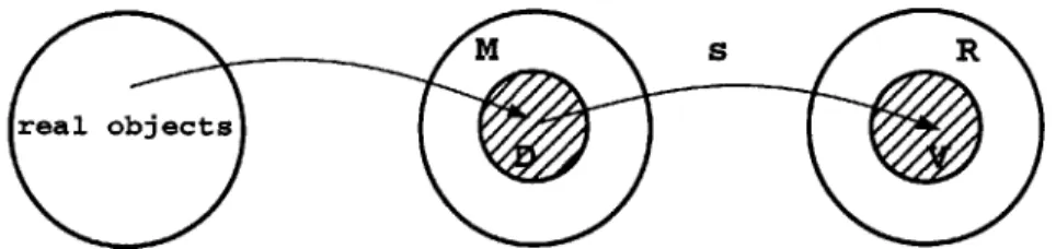
2-1 Domain and range of a representation scheme

3-1 3-2 3-3 3-4 3-5

Two valid solids . . . . Two invalid solids . . . . Three valid faces . . . . Two invalid faces . . . . Graph representation of the data structure . .

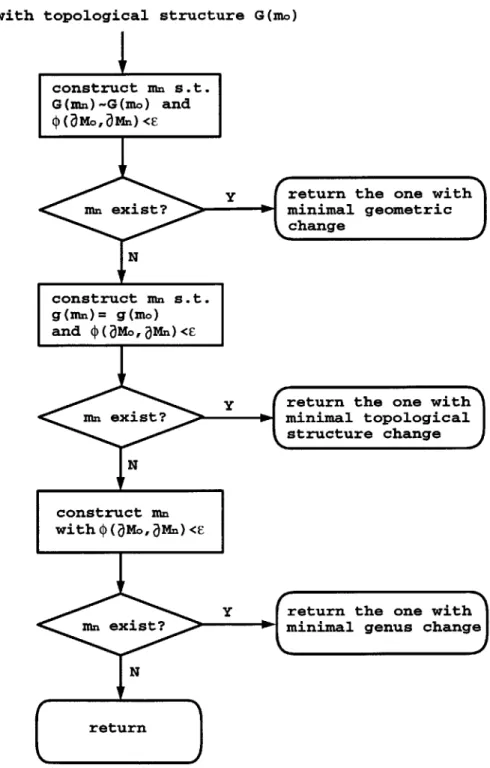
4-1 Flow1 chart of an id1II n roormcfr1 nrc+rm 4-2 4-3 4-4 4-5 4-6 4-7 4-8 4-9 5-1 5-2 5-3 5-4

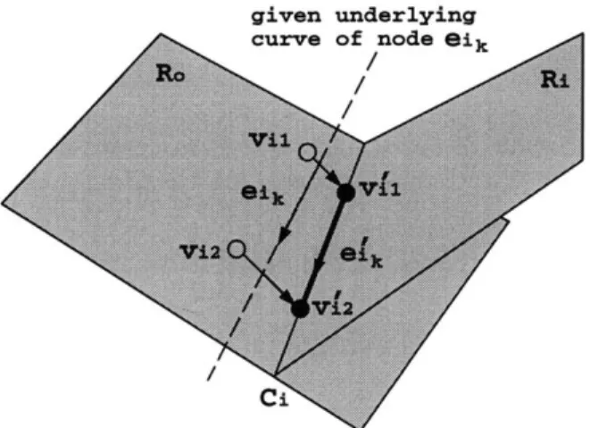
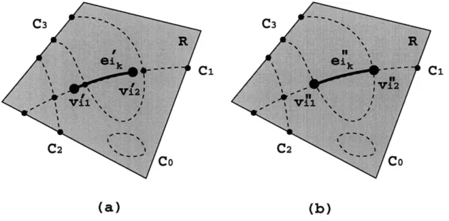
Two homeomorphic graphs with different geometric embeddings Curve segments from surface intersections . . . . Initial rectification of an edge on a face . . . . Creation of e' by vertex perturbation . . . . Trimming of dangling curve segments (a) and gap filling (b) Minimization of edge geometric change . . . . An instance of the restricted FR problem . . . . Illustration of the proof of Theorem 4.2.2 . . . .

An example of interval solid . . . . 2D version of condition C2 and C3 . . . . Influence of box sizes on approximate equality Boxes of an interval model . . . .

7 13 14 17 . . . . . 29 . . . . . 30 . . . . . 33 . . . . . 34 . . . . . 36 . . . 46 . . . 47 . . . 48 . . . 49 . . . 50 . . . 51 . . . 55 . . . 56 . . . 60 . . . . 6 5 . . . . 6 6 . . . . 6 9 . . . . 7 0

Exceptions to C 3 . . . . Illustration of Remark 5.3.1 . . . . Construction of 2D boxes satisfying the conditions in Remark 5.3.1 Construction of 3D boxes satisfying the conditions in Remark 5.3.1 5-5 5-6 5-7 5-8 6-1 6-2 6-3 6-4 6-5 6-6 6-7 6-8 6-9 6-10 6-11 6-12 6-13 72 73 74 76 . . . . 79 . . . . 83 . . . . 85 . . . . 86 2 . . 86 . . . . 90 . . . . 91 . . . . 93 . . . . 94 . . . . 96 . . . . 97 . . . . 98 4 m. . 98

7-1 Interval model as an internal model representation . . . . Examples of special surface intersection cases . . . .

Flow chart of box curve and box point identification . . . . Refinement of box curves formed by clusters . . . . Ordering of boxes in box curves of Example 2 . . . . Close-up of one box point in the parameter domain of Example Reconstruction of a vertex . . . . Gap closing in loop reconstruction . . . . Loop m odification . . . . Definition of the rotation index of a simple closed box curve Hole filling in shell reconstruction . . . . Part of a shaver handle . . . .

An invalid face with the resolution 10~6m . . . .

The face in Figure 6-12 becomes valid at the resolution 2 x

Chapter 1

Introduction

1.1

Motivation and Objectives

Model representation schemes enable man-machine and machine-machine communi-cation on product design and manufacturing. With semantic rules set by represen-tation schemes, models can be realized as physical artifacts. The success of such communication and realization, however, heavily relies on representational validity of models. That is, a model created using a specific modeling scheme should express de-sign intent unambiguously, and such intent can be faithfully interpreted by applying the same semantic rules without consulting the designer. A model is regarded as

in-valid if it corresponds to a model description which is not a mathematical abstraction

of any of the objects in the world under consideration

[53].

Constructive Solid Geometry (CSG) and Boundary Representation (B-rep) are the two representation schemes currently adopted by most solid modeling systems, see Mdntyld [45] and Hoffmann [29] for detailed descriptions of these two represen-tation methods. Both have great expressive power, capable of describing almost all man-made solids. CSG defines solids using primitive solids and operations such as regularized Boolean operations and transformations. A CSG model is generally represented as a CSG tree whose leaves are primitive solids and internal nodes are regularized Boolean operations and transformations. The solid is defined at the root

of the tree. Because primitives and operations are all well-defined, a CSG model is always valid if the tree is syntactically correct.

B-rep defines a solid by describing its boundary collectively. It uses topological boundary entities such as vertex, edge, loop, face, shell and region in a hierarchi-cal way. A higher level entity is defined by various lower level entities related by a certain structure, and at the top of this structure is the solid. Such a structure is often represented by a graph providing explicit information on adjacency and inci-dence relations of boundary entities. It also contains geometric information such as equations for points, curves and surfaces, each of which is associated to an appro-priate topological entity as its underlying geometry. Unlike CSG models, validity of rep models is not self-guaranteed. Indeed, "the fundamental problem with the B-rep database structure is the inability of the B-representation itself to guarantee object validity" [41]. Nevertheless, a B-rep model has the advantage of being an evaluated model. Boundary information necessary for important applications such as model rendering, analysis, and manufacturing, is readily available.

Invalid models may fail under certain modeling operations, generate useless re-sults in analysis programs, and produce defective products when used to compute control data to drive a manufacturing system. Model validity is becoming a promi-nent problem in data exchange as different CAD systems coexist even in one design or manufacturing unit. Model validity verification and rectification (or informally cor-rection) of invalid models, therefore, are very important problems in both modeling theory and CAD/CAM/CAE practice.

In the early years of solid modeling, validity verification was mostly done by the user, and was error-prone [53]. Model rectification was also done manually by experienced operators. The entire model verification and rectification process was laborious. As the complexity of models grows enormously, it becomes impossible for a human being to visualize defects and consistently repair them, and thus automated, or semi-automated with limited user assistance, model validity verification and defect rectification methods are needed in the solid modeling community, in order to design and manufacture defect-free products.

In this thesis, we focus on various aspects of the model verification and rectification problem. In particular, given a model, we try to answer the question "Is this model valid? If not, could it be fixed, and how?".

1.2

CAD Model Defects

Defects are those representational entities which violate semantic rules of modeling schemes. For a manifold B-rep model, mathematically, it is invalid if it does not describe a 2-manifold without boundary, and thus, represents a nonsense object in the modeling space.

At the representational level, there are two types of defects, topological errors and inconsistencies between topological and geometric specification. Topological errors refer to features in the incidence and adjacency graph which violate the manifoldness condition. For instance, if a face has no adjacent face through one of its edges, obviously, an arbitrary point on that edge does not have a 2-manifold neighborhood. Inconsistencies between topological and geometric specification refer to situations where a topological relation is inconsistent with the geometries of the topological entities involved in the relation. For instance, two faces sharing a common edge may be represented by two trimmed surface patches which do not meet properly at the geometry of the edge.

Visually, defects appear as gaps, dangling entities, inappropriate intersections, internal walls and inconsistent orientations. Gaps often exist along common edges between two faces. Such gaps may be extremely small and invisible in rendering, but may have disastrous effects on analysis and manufacturing applications. Models could also, but rarely, have considerable holes due to reasons such as missing patches. Inappropriate intersections are those intersections in the interior of a face. Internal walls subdivide solids into multiple regions, and are not allowed in a manifold B-rep model. Dangling entities could be dangling patches, edges, or isolated points, none of which define legitimate solids. Inconsistent orientations make the definition of interior and exterior unclear.

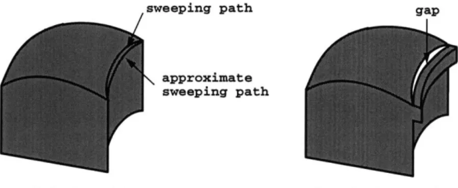
The causes of defects exist throughout the entire life cycle of a CAD model, es-pecially during model creation and data exchange. One major cause is pathological behaviors of certain geometric algorithms. For example, intersection curves are gen-erally approximated by lower degree curves. In Figure 1-1, a model is bounded by a set of B-spline surfaces. Later, a solid created by sweeping a planar shape along one of the edges is added. Since the edge is an intersection curve of high degree, the sweeping path is a B-spline curve approximating the edge and is not identical to the original edge. Therefore, there exists a gap between the boundary of the sweep-ing solid and the boundary of the original one1_{. Even if an algorithm is correctly} designed, poor implementation could still produce defects. For example, if the regu-larized union is not correctly implemented, it may leave an internal wall when applied to two cubes contacting each other at faces. Another major cause of defects is the precision limitation of the computer [30]. The computer can only represent a dis-crete domain of floating point numbers. Numbers unrepresentable in this domain are rounded to their closest floating point numbers. This causes computational errors, and such errors could accumulate to a fairly significant amount. In addition, CAD data will be shared by other systems or applications through data exchange. Since every system has its own proprietary data structure and internal accuracy/resolution for competitive purposes, useful information may be lost during the transmission. Therefore, a model valid in its native system may become invalid elsewhere.

An invalid model may fail under certain modeling operations. A typical example is the potential failure of point classification algorithms. A very fundamental query needed in Boolean operations is whether a point is inside or outside a solid. If the solid boundary has gaps, a ray casting algorithm will make a wrong decision if a selected ray shoots right through a gap. Modeling operations which rely on such decisions, thus, may fail to perform properly, or even lead to system error, if they are unable to handle contradictions or ambiguities induced by wrong decisions. Downstream

'Although the size of the gap can be reduced by increasing the approximation precision, such actions will create B-spline surfaces with very long knot vectors, which will affect the performance and robustness of downstream applications. In general, current solid modeling systems balance the approximation precision and the complexity of resulting models.

/sweeping path

approximate

sweeping path

original model after Boolean union

Figure 1-1: Gaps created by adding a sweeping solid

applications are also vulnerable to defects. A finite element analysis program may return useless results if the input mesh is created using a CAD model with gaps. Without proper post-processing, NC data computed from such models will leave defects such as under-cuts in finished products. In rapid prototyping, an internal wall will cause uneven material shrinkage at the location and subsequent warping and loss of part accuracy [12]. A model with inconsistent orientation will visually have black faces during rendering. Defects may be further exaggerated through data exchange. A model may become completely unrecognizable in the receiving system, and cost tremendous man-power and financial resources to fix. See a very good example in Figure 1-2, where the left image is the model in the native system and the right is in the receiving system. Such failures of data exchange are due to different tolerances used in the sending and the receiving systems and/or that the model representation used in the sending system does not contain topological information, see [36].

A recent report to NIST [16] indicates that the interoperability problem of CAD data costs the US automobile industry and its part sub-contractors over one billion dollars a year, including investment in avoiding such problems before data exchange and fixing problematic data afterwards and profit loss due to delay in design and production. Although much can be accomplished via proper widespread use of the STEP standard [65] in reducing the magnitude of the interoperability problem, many of data exchange problems and data quality problems categorized in the NIST report

Figure 1-2: An example of failure in data exchange [36]

are directly or indirectly related to model validity.

1.3

Thesis Organization

Chapter 2 provides the necessary background of this thesis. It contains a brief in-troduction of solid modeling theory, especially on model validity. It also provides a literature review of recent research on model verification and rectification, espe-cially on triangulated models. Another approach to the model validity problem, cur-rently explored by many, is the development of robust geometric representations as replacements of traditional representations using floating point specification. Interval geometric representation, which will be used in this work, is introduced briefly.

Chapter 3 provides mathematical fundamentals of ideal boundary models and studies validity of ideal B-rep models. It defines solid modeling concepts such as solid, shell, face, loop, edge, and vertex, as well as loop and face orientations. It then derives conditions for manifold B-rep model validity and proves their sufficiency. Such conditions are useful in developing model verification and rectification methods. Chapter 4 analyzes the nature of the boundary rectification problem, and proposes a rectify-by-reconstruction approach. It also proves that the boundary reconstruction problem, which searches for a global consistent and optimal boundary model on the underlying surfaces of a given model, is NP-hard.

et al [33, 34]. In particular, it defines the concept of approximate equality relation between an interval solid model and the intended ideal model, and derives sufficient conditions for such approximate equality.

Chapter 6 presents a model rectification methodology based on our study of the problem in Chapters 4 and 5. This method builds a valid model in the neighborhood of the object described by a traditional boundary representation model with float-ing point specification. It converts an erroneous model into an interval solid model, guaranteed to be gap-free. The chapter also provides necessary techniques for con-structing interval solid models, such as box size control, data reduction, and ordering boxes. An example illustrates our methodology for robust conversion.

Chapter 7 concludes the thesis with a summary of contributions and recommen-dations of future research. In particular, we propose the use interval model represen-tation as an internal represenrepresen-tation at the core of solid modeling systems, and explain how this representation will benefit the development of robust application algorithms. Appendix A provides a brief introduction to the theory of NP-completeness, needed in Chapter 4. Appendix B derives the recursive formulae for evaluating an interval point on an interval B-spline curve or surface using de Boor's algorithm, and the approximate relation between the size of such a point and its parameter resolution, all needed in Chapters 5 and 6.

Chapter 2

Literature Review

2.1

Manifold B-Rep Model Validity

Fundamental concepts and definitions of solid modeling can be found in Requicha [53], Mintyli [45], Hoffmann [29], Braid [14], and the literature cited therein. A historical overview of solid modeling developments can be found in Braid [13] and Voelcker and Requicha [66]. This section provides a brief summary of prior research work on model validity, especially of manifold B-rep models.

A solid modeler is designed to model a set of mathematical solids, which form the modeling space M of the modeler. Each element in M is an abstraction of a real solid. A modeler consists of representations and a representation scheme. A representation is a finite symbol structure constructed from an alphabet according to syntactical rules. All syntactically correct representations form the representation space R. A representation scheme is defined as a relation s : M -+ R, whose domain

D C M and whose range V C R. A valid representation is a representation in V, see

Figure 2-1, Requicha [53] and Mintyli [45].

Manifold B-rep describes real solids whose mathematical abstractions are r-sets with 2-manifold boundary [53, 45]. An r-set is a bounded, regular and semianalytic subset in E3. Almost all man-made solids can be represented by such mathematical

descriptions. B-rep uses a collection of 2-dimensional entities, called faces, properly connected and consistently oriented, to define solid boundaries. Each face is bounded

S

Figure 2-1: Domain and range of a representation scheme

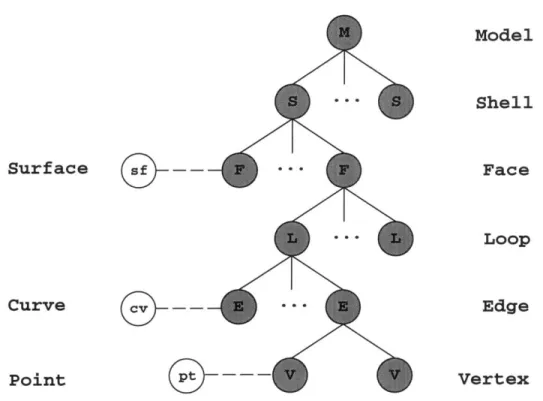
by loops and is embedded on a surface. Each loop is a string of edges, properly connected and consistently oriented to form a simple closed curve with orientation. Each edge is a simple open or closed curve, and embedded on a curve and bounded by two vertices. In addition, a shell is defined as a collection of faces whose union is a connected 2-manifold without boundary. See Figure 3-5 for the diagram of such a hierarchical structure. Adjacency and incidence relations of these topological entities are referred to as "topology" or topological structure, and their underlying geometries as "geometry" or geometric representation.

A B-rep model is valid if its faces form a 2-manifold without boundary. Specifically, a B-rep model is valid if the following conditions are satisfied [44]:

1. Faces may intersect only at common edges or vertices. 2. Each edge is shared by exactly two faces.

3. Faces around each vertex can be arranged in a cyclical sequence such that each consecutive pair share an edge incident to the vertex.

Similar conditions were also presented in terms of a simplicial complex methodology in Hoffmann [29]. The above conditions for validity require topological integrity, meaning that it is possible to assign each topological entity a well-behaved geometry such that the overall geometry is a 2-manifold without boundary [44], and geometric integrity, meaning that geometric representation conforms to all topological relations presented in the topological structure [15]. Orientations of faces must obey Moebius'

Topological integrity can be assured by using Euler operators as primitive mod-eling operators. Euler operators were introduced by Baumgart [9] in his work on computer vision, and were extensively studied by many others [21, 14, 15, 46, 44], see also Braid [13] for historical notes on Euler operators. The theoretical basis is the well-known Euler-Poincar6 formula, which holds for polyhedra in E3. A limited set of Euler operators is enough to construct any polyhedron. For convenience, often an augmented set of Euler operators is chosen. Higher level modeling operations, such as sweeping, chamfering, and set operations, are developed along with geometric specification and computation algorithms.

In Braid et al [15], a topological structure is called admissible if certain conditions are satisfied, mainly the Euler-Poincar6 formula. Admissibility does not imply validity because the Euler-Poincare formula is necessary but not sufficient, meaning that a polyhedral model satisfying this formula may not be a 2-manifold [14, 15, 29]. Mdntyld

[44]

Geometric integrity can be verified by two tests, see [15] for polyhedral models. Local test verifies if underlying curves of edges and coordinates of vertices are con-sistent with surfaces. Global test checks if there are any surface intersections in the interiors of faces.

2.2

CAD Model Rectification

This section reviews model rectification techniques, mainly on polyhedral models and surface models. Very little research on curved B-rep model verification and rectifica-tion has been published. Some commercial software is now marketed including model verification and rectification tools. Without access to their proprietary techniques, their review is superficial. Based on descriptions of product features [37, 36, 38], such software tools detect and rectify local defects. Global consistency is left to the user

or processed in an iterative manner.

2.2.1

Polyhedral models

Polyhedral models use linear geometries as underlying geometries of boundary enti-ties. Though limited in expressive power, they are widely used to approximate curved objects in model rendering, finite element analysis, and manufacturing such as rapid prototyping.

A special class of polyhedral models is triangulated models such as STL models in rapid prototyping. Despite of its many drawbacks, STL file format [1] is the de

facto industry standard for solid freeform fabrication as a method for rapid

prototyp-ing. An STL model contains a collection of unordered triangles with no topological information. Each triangle is represented by three points as its vertices and a normal vector indicating orientation. Therefore, the boundary of a solid is defined by con-sistently oriented and properly connected triangles. Defects in STL models are gaps, inappropriate intersections, dangling triangles, overlapping triangles, and inconsistent orientations [12, 43].

Bohn and Wozny [12] proposed an algorithm which detects and repairs gaps in STL models. It first identifies lamina edges. A lamina edge on a triangle is an edge which has no adjacent triangle, or more than one adjacent triangles, or one adjacent triangle with inconsistent orientation. The algorithm then strings lamina edges into a directed graph, and separates the graph into a collection of simple closed curves. Complicated situations where such separations are ambiguous are resolved using topological and geometric heuristic rules, such as the assumption that a model only represents one solid. These simple closed curves bound holes. Additional triangles are added to close holes.

Mdkeli and Dolenc [43] developed methods for efficiently repairing STL defects, including gaps, overlapping or duplicate triangles, and intersecting triangles. The algorithm first detects adjacency relations among triangles. Before a triangle is in-serted into a specially designed data structure, each of its vertices is compared with the vertices of triangles already in the data structure, and merged with the closest

one, if the distance is within a given tolerance. Neighboring relations are then de-tected. Edges without matching edges from other triangles are classified as erroneous edges. Gaps bounded by such edges will be triangulated. Degenerated triangles and exact duplicates are deleted at this stage. The orientation of a triangle is determined by the number of intersections between the model and a ray emitted from one of the vertices in the direction of the normal vector. Intersections are checked within one connected component and between different components.

The above algorithms succeed in the majority of candidate models. However, as local methods, global consistency is not guaranteed. Unwanted features may be added during gap-filling. In addition, triangles added to fill in gaps are often ill-shaped and inappropriate for some analysis and manufacturing programs.

Barequet and Sharir [8] developed a global gap-closing algorithm for polyhedral models, using a partial curve matching technique. In their method, gap boundaries are discretized. Each match between any two parts of gap boundaries is given a score based on the closeness of their discrete points. They have shown that finding a consistent set of partial curve matches with maximum score, a subproblem of their repairing process, is NP-hard. Barequet and Kumar [7] developed a model repairing system using the algorithm in [8], but with a modified score which is the normalized gap area between two matched parts of gap boundaries. Visualization tools were also provided to enable the user to override unwanted modifications. The system was improved by Barequet et al [6] in terms of efficiency, and extended to models with regular arrangement of entire NURBS surface patches. However, this extension does not handle trimmed patches with intersection curve boundaries and real B-rep models involving non-regular arrangement of surface patches.

A different type of global algorithm is based on spatial subdivision. Murali and Funkhouser [51] developed an algorithm which handles defects such as intersecting and overlapping polygons and mis-oriented polygons. The algorithm follows three steps: spatial subdivision, solid region identification, and model output. It first subdivides R3

into convex cells using planes on which polygons sit. A cell adjacency graph is then constructed. Each node is a convex cell, and each arc is a link between two cells

sharing a polygon. Whether a cell is a part of the intended solid is determined by its solidity value, ranging from -1 to 1. The solidity value of a cell is computed based on how much area of the cell boundary is covered by original polygons as well as solidity values of neighboring cells. Boundary polygons of cells with positive solidity values are then output as the resulting solid boundary. A major advantage of this algorithm is that it always outputs a valid solid. One limitation of this algorithm is that it may mishandle missing polygons and add cells which do not belong to the model.

2.2.2

Surface models

Surface models are also boundary models. Solid boundaries are defined by surface patches with no topological information. As patches often mismatch for reasonably complex models, validity is difficult to achieve and maintain.

Hamann and Jean

[27]

control points of neighboring patches. The method is a geometric approach with a few topological constraints. It may created non-manifold features due to missing patches and surface intersections. Trimmed patches may impose some difficulties on boundary specification for Coons patch approximation. Continuity will change if a specified boundary curve is located inside a surface patch. In addition, subdivision of surfaces into quadrilateral patches burdens the user. Although user interference is unavoidable as the authors believe, it should be minimized.

Hu and Sun [35] developed an algorithm which closes numerical gaps between two trimmed patches by moving one surface towards one of the trimming curves of the other surface. This method corrects gaps up to a certain accuracy, and gaps

will reappear when higher accuracies are used in application programs. Moreover, it perturbs the control points of a surface so that one specific trimming curve on the surface is close to a target curve in the space. Since this method changes surfaces, it may not be suitable for surfaces specifically designed to meet functionality and performance requirements.

A better approach to surface model rectification first involves construction of the topological structure. This not only rectifies an invalid model, but also converts surface models into B-rep models [59].

Evensen and Dokken [23] developed an adjacency analyzer for transferring ge-ometries between different CAD systems. The adjacency analyzer reconstructs the topological structure of a model whose original topological structure is either modified or completely lost during data exchange. The underlying algorithm uses a geometric resolution to find possible common intervals between two curves. The adjacency test of surfaces examines the closeness of boundary curves of any two surfaces in a sur-face model using the given resolution. Sursur-faces with their boundary curves sharing common intervals are tagged as adjacent. As the authors pointed out, the analyzer is unable to handle trimmed surfaces, two surfaces intersecting in their interiors, and overlapping surfaces. More importantly, the algorithm only constructs local topology, i.e. incidence and adjacency relations among surface patches, without verifying global topology.

Sheng and Meier [59] developed a topology analyzer for generating topological structures for surface models. The algorithm first discretizes boundary curves of surface patches, and then identifies matching pairs of boundary curves if any two curves fall inside small neighborhoods of each other. The matching polygonal curves are merged and the two corresponding patches are considered adjacent. This is, indeed, very similar to the algorithm developed by Barequet and Sharir [8], but without consideration of global topological correctness and geometric optimality.

2.3

Robust Geometric Representation

Another direction towards robust solid modeling, currently investigated by many, is to develop robust geometric representations in the floating point environment. Such a representation is often based on a certain arithmetic system whose numbers are representable on the computer and operations are closed. Floating point representa-tion has a discrete domain of numbers, and round-off is unavoidable [30]. The goal of robust geometric representations is to maintain consistency of topological decisions based on geometric computations, so that models could achieve topological correct-ness and geometric consistency at least at a certain level of credibility. Two typical classes of representations are of great interest: integer-based and error-bounded.

Integer-based representations use integer numbers. Pure integer representations use a certain data structure to store an integer. Values and coefficients for the geomet-ric representation are all integers. If the result of a computation procedure requires more bits, the data structure may have a mechanism for dynamically growing storage size. As uncontrolled growths may lead to system failure, in general, such a result is replaced by an approximant. For example, an intersection point between two lines, is approximated by the closest point in the grid of representable integer points. Rational arithmetic represents all numbers as fractions with both numerator and denominator stored as integers. At present, rational arithmetic is inefficient when used in geomet-ric computations, and thus, is infrequently used for geometgeomet-ric modeling. It may be used in situations where exact evaluations are crucial. In so-called lazy arithmetic, evaluations are performed using error-bounded methods, and switched to rational arithmetic when approaching degeneracies. See [47, 24, 39, 40, 10, 3] for references on integer, rational and lazy arithmetic and their applications in geometric and solid modeling. In the following, we review a typical error-bounded representation, interval

geometric representation, since it will play a key role in our approach to the model

verification and rectification problem.

In interval arithmetic [49, 4], a number is a closed interval in R, and algebraic operations are well-defined and closed. If input values to a computation procedure

are known to be intervals, interval evaluation returns intervals containing the exact result. By using rounded interval arithmetic, even round-off errors can be captured, and enclosures of exact results are computationally preserved [2]. However, both interval and rounded interval arithmetic are conservative, meaning that width growth may be unnecessarily larger than actual error propagation. Therefore, width control is a very important issue in algorithms using interval arithmetic.

Interval geometric representation uses interval numbers for parameters and coef-ficients, and in general, represents a 3D region in space. An interval geometry also represents a family of geometries of the indicated dimensionality. For instance, an interval curve may refer to its induced region in the setting of point-set theory, or to a family of curves when its dimensionality is of primary interest. Interval polynomials were used in numerical analysis since the 1960's [49]. Interval B6zier curves, whose control points are rectangular boxes and represented as interval vectorsi, were first studied and applied by Sederberg and Farouki [57] in curve approximation. Interval explicit B-spline surfaces were studied by Tuohy and Patrikalakis [63, 64] and ap-plied in approximation problems. Tuohy et al [62] extended the concept to interval parametric B-spline surfaces and applied it in surface approximation. Shen and Pa-trikalakis [58] studied the numerical and geometric properties of interval B-splines. Hu et al [33, 34] first proposed an interval solid modeling method. It uses interval points, curves and surfaces as underlying geometries for vertices, edges and surfaces. A graph-based data structure incorporating special features of interval geometries was also developed to represent both manifold and non-manifold objects. Algorithms of Boolean operations are based on robust interval curve and surface intersection algo-rithms [32, 31]. These rely on the Interval Projected Polyhedron (IPP) algorithm for robustly solving a system of m nonlinear polynomial equations in n unknowns within an n-dimensional rectangular box, see Sherbrooke and Patrikalakis [60] and Abrams et al [2]. However, topological properties of interval solid models were not studied in the above references. Topological issues are very important. As an interval solid model defines a family of boundaries, topological invariance of members is crucial

for retrieving correct boundary information from the interval model. We study such issues in detail in Chapter 5.

Chapter 3

Representational Validity of

Boundary Representation Models

3.1

Mathematical Preliminaries

A real solid is a material object that occupies a region in 3-space. An abstract solid, therefore, must unambiguously describe the region occupied by the solid, so that it is possible to classify whether a point is inside the region of the solid [54]. Another important characteristic of a real solid is its physical realizability, which refers to the possibility of rebuilding it [52]. On the other hand, this realizability should not be limited by current manufacturing technology.

A widely accepted definition of solid was given by Requicha [53]: "a solid, denoted as r-set, is a subset of R3 _{that is bounded}1_{, closed}2_{, regular}3 _{and semianalytic}4_{. This} definition captures mathematical characteristics of most real solids of interest, such as mechanical parts. However, this definition allows non-manifold features, such as the contacting edge between two cubes, a feature which is non-manufacturable (see

1_{A set in R}3 _{is bounded if for every pair of points in this set, the distance is less than some} number [50].

2_{See the definition in this section.}

3

A set in R3 is regular if it equals the closure of its interior [53]. 4

A set is semianalytic if it can be expressed as a finite Boolean combination of sets of the form

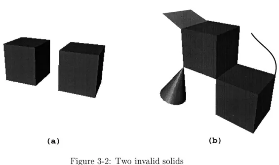
Figure 3-2(b)). It is for that reason that many prefer a solid to be a topological manifold [451.

In the following we state some definitions pertinent for this discussion. For a reference see [18, 20, 48].

Let p E R' and let r > 0. The open ball B(p, r) of radius r centered at p is defined as the set of points x

C

open if for every point a E A there exists an r > 0 so that B(a, r) C A. A subset A

of R" is called closed if its complement -,A is open.

A k-simplex o-T=conv(T) is the convex hull of an affinely independent set T C R",

TI = k + 1, where |TI denotes the number of elements of T. k is called the dimension

of the simplex aT. A simplicial complex K is a finite collection of simplices that satisfy the following:

1. if uT E K then c-u E K, VU CT, and

2. if u, o-v E K, then -unv = O-u n a-v.

The underlying space of K is [K] = UCEK U-, with the induced topology from R".

A subcomplex of K is a simplicial complex L C K.

Definition 3.1.1 Let A C Rn. The interior Int(A) of A consists of all points a E A

such that A contains a neighborhood of a. The closure A is defined as A = ,int(-,A).

The boundary of A is Bd(A) = A-Int(A). A shall be called compact if it is bounded

and closed.

Definition 3.1.2 Let A1, A2 be subsets of R', R', respectively, and let g : A1 -+ A2

be a map. We say that g is continuous, if for every point b E A2 and r > 0, the

inverse image of B(b, r) n A2 is equal to C n A1, where C is an open set in Rn. In

addition, we say that g is a homeomorphism if g is 1-1, onto and g and g 1 _{are both}

Definition 3.1.3 Let M, N be subsets of R'. We say that M is a n-manifold

(with-out boundary) if every point p

C

N is defined as the set of points x E N that have a neighborhood homeomorphic to

Rn+, and the interior Int(N) as the set of points x

e

homeomorphic to R'.

In view of the above, we define an open disk A = Int(M), where M C R3 is a 2-manifold (with boundary) homeomorphic to the unit closed disk D ={x

C

R2I|xjj < 1}. A half open disk Ah is a bounded subset of R3 _{homeomorphic to}

{x = (xI, x2)

c

Definition 3.1.4 Let M be an n-manifold, with or without boundary. If there exists

a simplicial complex K whose underlying space [K] is homeomorphic to M, then M is said to be a triangulated n-manifold, and K is called a triangulation of M.

Remark 3.1.1 If N is a n-manifold with boundary, then its boundary ON is an

(n - 1) manifold without boundary. For a proof see [26], p. 59.

Definition 3.1.5 A curve c C Rn is the image of a continuous map g : [0, 1] -+ R".

It is called simple if g is 1-1 over (0,1). c is closed if g(0) = g(1). We also say that c has a self-intersection if g(to) = g(ti), with to

#

Definition 3.1.6 A (parametrized) surface E is the image of a continuous map (D D c R2 -+ R3 _{. We can write}

<b(u, v) = (x(u, v), y (u, v), z(u, v)).

If (D is differentiable, we call E a differentiable surface. In that case we say that E

is smooth at a point (uo, vo) if the vector 2 x '-

#

of measure zero. Finally, we say that E has a self-intersection if there exist points

(u1, v1)

#

3.2

Solids and their Boundaries

In view of the above and [53, 45], we may now define:

Definition 3.2.1 Let S C R3. S shall be called a solid

nected 3-manifold with boundary, so that:

if it is a compact and

con-1. Its boundary 0S is a 2-manifold without boundary, and

2. OS C U> Rj, where {Rj} are AS surfaces.

Figures 3-1 and 3-2 illustrate several valid and invalid solids.

Figure 3-1: Two valid solids

Obviously, for a solid S we have OS = S - int(S). In addition, thanks to a

result from geometric topology, we note that a solid is a triangulable manifold with boundary, and thus it is orientable [48]. Roughly speaking, the latter means that we know precisely its interior as well as its exterior. Notice, also, that the boundary of a solid may not be connected if the solid has cavities.

Definition 3.2.2 Let S be a solid. A shell C of S is a connected component of

9S [44]. For such a C, we define the inner (outer) part of C, C'(C0 ), as the interior

(a) (b)

Figure 3-2: Two invalid solids

Notice that since C is a 2-manifold without boundary sitting in R3_{, it is orientable,} and thus R3 - C has precisely two connected components, one bounded and one

unbounded.

Remark 3.2.1 Let S be a solid. Then, there exists a unique shell Ce, called external

shell, so that every other shell of S is contained in its inner part CeI.

Proof: Let U be the unique unbounded connected component of R3 - S. Let now

Ce be a shell of S with the property that some point p E Ce has a neighborhood that

does not meet any other shell of S and intersects U. Since Ce is orientable, we see that every point of Ce has the above property. We now claim that this shell of S is the only one with this property; for otherwise, S would not have been connected. Finally, if C is another shell of S it obviously lies in the inner part of Ce, since the outer part of Ce is precisely U.

All shells of S, except Ce shall be called internal. Note from the above remark that

k

S = UeI - C C1 (3.1)

i=i1

We next define the so-called faces of a solid, in order to achieve a boundary representation of solids. Face can be defined in an analogous way to a solid, see Mintyli [44]. The following definition gives a clear description of face topology.

Definition 3.2.3 A face f of a solid S is a non void subset of OS having the following

properties:

1. f is a subset of one, and only one, AS surface.

2. The interior Int(f) in OS is a connected 2-manifold, and

3. f is homeomorphic to a (topological) sphere E minus a finite number of mutually

disjoint (nondegenerate) open disks Ai C E, i = 0,1 .. , k, k > 0, so that for

i

#

j,

n

azj

The requirement that a face is embedded in one surface is representational rather than mathematical. This also makes an abstract face close to a natural face, which in general is bounded by natural edges manifested by tangential discontinuities. It is also accepted in solid modeling practice that a face has no handles. Indeed, this is the case as definition 3.2.3(3) shows. Notice that a face is path-connected, and the connectedness of its interior excludes two neighboring faces to be taken as one face. See also Mintyli [45].

The following remark comes directly from definition 3.2.3 and is useful for face representation.

Remark 3.2.2 Let f be a face of a solid S, and k > 0 be as in definition 3.2.3(3).

Then,

" f is homeomorphic to F, where F is the closed unit disk D = Do minus k

mutually disjoint (nondegenerate) open disks Di, so that Di C D, for all 1 <

i < k, and aDi

n

_#

and

Proof: Indeed, a sphere E minus the open disk A0 is (homeomorphic to) the disk D.

Further exclusion of the remaining open disks Ai, 1 < i < k results in the description of F in the first bullet. To prove the second assertion let us suppose that C1, C2 are

two different connected components of F. Then, we may pick a simple closed curve

c E Bd(C1) so that its interior is just C1. This, however, is a contradiction to the

second bullet.

We define the boundary of

f

f

between

f

f

f

f

Bd(f) = g-1(OD) U

U

The following remark describes the topology of Bd(f).

Remark 3.2.3 Let x C Bd(f), and let Ai be an open disk so that x C OAi. Then, we may choose r > 0 so that

Fl. ci = B(x, r) n aA is a simple curve. Moreover, if x E DAj,

j

F2. f

n

nT

OAi.

n

More-over, UL'i, {D'(f) U A} = E n B(x, r).

Proof: Fl. Let x

C

Ai. Since that boundary is an 1-manifold without boundary, that is, a simple closed curve, we may pick an r > 0 so that ci = B(x, r)

n

x E &aj,

j

n

n',

n

al, a2. Since each Ai is a 2-manifold with boundary the simple closed curve ai,

Since ci

n

contain the points a., a., and a?, a!+, respectively. The proof is now complete. *

Definition 3.2.4 Let f, F, g be as above. A loop of f is one of the simple closed

curves g-1(DD) and g-'(Di).

We may now define the notions of external/internal loops of a face

f.

f,

above. We define the external loop of

f,

other loops Li of

f

a face is not unique, we may use that notion to 'reconstruct' a face from its boundary loops. To achieve the latter, we will have to define the notion of a region bounded by a loop in

f.

k

f = Re -

U

i=1

Notice the similarity of the above formula, with formula (3.1). Figures 3-3 and 3-4 illustrate several valid and invalid faces.

(a) (b) (c)

Figure 3-3: Three valid faces

We may now expand the above discussion of the notion of the 'region bounded by loops' so that we can use it in the next section. Let E : <D : [0, 1] x [0, 1] - R3 be an AS surface and let cj,

j

n

(a)

Figure 3-4: Two invalid faces

a specific orientation. Then, it is possible to define the region bounded by the closed

curves c3, R'. To do that, we consider the curves l = -1 (cj). Then, since D is 1 -1

over Nj, each l is a simple closed curve.

The given orientation(s) on E and cj induce-via 4 1-an orientation on [0, 1] x [0, 1] and each l. We can then agree that each of the above oriented closed curves define a region in [0,1] x [0,1]. For each lj we define the region bounded by l, R(l) as the subset of [0, 1] x [0, 1] that lies to the left of l as one is walking on the positive side of [0, 1] x [0, 1], along lj with respect to its orientation. Finally, we define

RE= R* = nj4(R(lj)), if Bd(R*) = Ujcj and R* is connected (3.4)

0 otherwise

Now, a loop can be decomposed into edges.

Definition 3.2.5 An edge e of a face f is a subset of Bd(f) such that

1. It is also a subset of a loop, and

2. It is homeomorphic to either a simple closed curve or to an open simple curve.

On the other hand, edges are bounded by vertices:

Definition 3.2.6 A vertex v of an edge e is " A component of Bd(e), if Bd(e)

#

" An arbitrary point in Bd(e) if Bd(e) = 0.

In general, the underlying geometry of an edge is the intersection curve of the two underlying surfaces of the two faces sharing this edge, and a vertex is the intersection of three or more surfaces.

We next give the definition of boundary representation:

Definition 3.2.7 A boundary representation of a solid S is a collection of faces

fi,

1. U -f= OS, and

2. For any i 0 j, fi n fj = Bd(fi) n Bd(fj).

3.3

Representational Validity Conditions

3.3.1

Data structure

A typical data structure for B-rep model has a graph structure as shown in Figure 3-5. B-rep data structures can be found in Baumgart [9], Mantyli

[45],

1. A vertex node is the representation of a vertex. It has a pointer to a node containing Cartesian coordinates.

2. An edge node is the representation of an edge. It has two ordered pointers to two vertex nodes, and a pointer to a node containing the geometric representation of a curve, including a binary field specifying the orientation of the edge with respect to the orientation of the curve.

3. A loop node is the representation of a loop. It has a collection of pointers, each of which points to an edge node and has a binary field specifying the orientation of the edge in the loop with respect to the orientation of the edge.

4. A face node is the representation of a face. It has a collection of pointers, each of which points to a loop node and has a binary field specifying the orientation of the loop in the face with respect to the orientation of the loop. It also has

a pointer to a node containing the geometric representation of an AS surface (see Defintion 3.1.6), including a binary field specifying the orientation of the face with respect to the orientation of the AS surface.

5. A shell node is the representation of a shell. It has a collection of pointers to face nodes. Model Shell Surface -- Face -. -- _Loop Curve Edge Point

--

Figure 3-5: Graph representation of the data structure

The data structure is an adaptation of the STEP file structure [65], and is able to hold non-manifold features, as we assume a given representation could be topologically incorrect.

3.3.2

Sufficient conditions for node validity

Representational validity verification, for a certain data structure like the one in sec-tion 3.3.1, is a process of verifying that each node in an instance of the data structure is a valid representation of the corresponding topological entity. The following