HAL Id: hal-00866442
https://hal.archives-ouvertes.fr/hal-00866442
Preprint submitted on 30 Sep 2013
HAL is a multi-disciplinary open access
archive for the deposit and dissemination of
sci-entific research documents, whether they are
pub-lished or not. The documents may come from
teaching and research institutions in France or
L’archive ouverte pluridisciplinaire HAL, est
destinée au dépôt et à la diffusion de documents
scientifiques de niveau recherche, publiés ou non,
émanant des établissements d’enseignement et de
recherche français ou étrangers, des laboratoires
Assessing and ordering investments in polluting
fossil-fueled and zero-carbon capital
Oskar Lecuyer, Adrien Vogt-Schilb
To cite this version:
Oskar Lecuyer, Adrien Vogt-Schilb. Assessing and ordering investments in polluting fossil-fueled and
zero-carbon capital. 2013. �hal-00866442�
No 49-2013
Assessing and ordering investments in
polluting fossil-fueled and zero-carbon
capital
Oskar Lecuyer
Adrien Vogt-Schilb
July 2013
Assessing and ordering investments in polluting fossil-fueled and zero-carbon capital
Abstract
Climate change mitigation requires to replace preexisting carbon-intensive capital with different types of cleaner capital. Coal power and inefficient thermal engines may be phased out by gas power and efficient thermal engines or by renewable power and electric vehicles. We derive the optimal timing and costs of investment in a low- and a zero-carbon technology, under an exogenous ceiling constraint on atmospheric pollution. Producing output from the low-carbon technology requires to extract an exhaustible resource. A general finding is that investment in the expensive zero-carbon technology should always be higher than, and can optimally start before, investment in the cheaper low-carbon technology. We then provide illustrative simulations calibrated with data from the European electricity sector. The optimal investment schedule involves building some gas capacity that will be left unused before it naturally depreciates, a process known as mothballing or early scrapping. Finally, the levelized cost of electricity (LCOE) is a misleading metric to assess investment in new capacities. Optimal LCOEs vary dramatically across technologies. Ranking technologies according to their LCOE would bring too little investment in renewable power, and too much in the intermediate gas power. Keywords: levelized costs of electricity; lifecycle cost; climate change mitigation; path dependence; technology policy; optimal timing; capital utilization rate
JEL classification: O21, Q32, Q41, R4, Q54, Q58
Évaluation et séquençage des investissements dans du capital bas carbone et zéro carbone
Résumé
La transition vers une économie bas carbone nécessite de remplacer le capital existant, très émetteur de gaz à effet de serre (GES), par du capital partiellement ou totalement décarboné: les centrales à charbon peuvent être remplacées par du gaz de dernière génération ou des renouvelables, les véhicules thermiques inefficaces peuvent être remplacés par des véhicules thermiques efficaces ou des voitures électriques. Nous étudions le profil optimal d'investissements dans des technologies bas carbone et zéro carbone pour remplacer un stock existant de capital polluant, sous contrainte d'un plafond sur les émissions cumulées, et lorsque produire grâce à la technologie bas carbone requiert l'extraction de ressources fossiles. Nous trouvons que la technologie zéro carbone doit toujours être construite à un coût plus élevé que la technologie bas carbone, et que les investissements zéro carbone peuvent commencer avant les investissements bas carbone. Nous réalisons ensuite une simulation numérique calibrée sur le secteur électrique européen. Nous trouvons que la transition optimale vers un secteur électrique bas carbone impose d'investir dans des centrales à gaz qui seront par la suite sous-utilisées ("mise sous cocon"). Finalement, le coût actualisé de l'électricité (CAE) n'est pas un bon indicateur pour comparer les technologies. Classer les technologies par leur CAE induiraient trop d'investissements dans les centrales à gaz, et pas assez dans les renouvelables. Mots-clés : coûts actualisés de l'électricité; dépréciation; atténuation du changement climatique; dépendance au sentier; politiques technologiques; timing optimal; taux d'utilisation du capital.
Assessing and ordering investments in
polluting fossil-fueled and zero-carbon capital
Oskar Lecuyer1, 2,∗, Adrien Vogt-Schilb1
1CIRED, 45 bis, avenue de la Belle Gabrielle, 94736 Nogent-sur-Marne Cedex, France 2EDF R&D, 1 Avenue du G´en´eral de Gaulle, 92141 Clamart Cedex,France
Abstract
Climate change mitigation requires to replace preexisting carbon-intensive cap-ital with different types of cleaner capcap-ital. Coal power and inefficient thermal engines may be phased out by gas power and efficient thermal engines or by renewable power and electric vehicles. We derive the optimal timing and costs of investment in a low- and a zero-carbon technology, under an exogenous ceil-ing constraint on atmospheric pollution. Producceil-ing output from the low-carbon technology requires to extract an exhaustible resource. A general finding is that investment in the expensive zero-carbon technology should always be higher than, and can optimally start before, investment in the cheaper low-carbon technology. We then provide illustrative simulations calibrated with data from the European electricity sector. The optimal investment schedule involves build-ing some gas capacity that will be left unused before it naturally depreciates, a process known as mothballing or early scrapping. Finally, the levelized cost of electricity (LCOE) is a misleading metric to assess investment in new capacities. Optimal LCOEs vary dramatically across technologies. Ranking technologies according to their LCOE would bring too little investment in renewable power, and too much in the intermediate gas power.
Keywords: levelized costs of electricity; lifecycle cost; climate change mitigation; path dependence; technology policy; optimal timing; capital utilization rate
JEL classification: O21, Q32, Q41, R4, Q54, Q58
1. Introduction
The European Union aims at decarbonizing almost completely the power sector by 2050, and at reducing emissions from transportation by two thirds below the 1990 level by 2050 (UE, 2011). This requires that in both sectors, the preexisting carbon-intensive capital is replaced by one or several types of greener technologies. Cutting emissions from existing coal power plants can for instance be achieved by building gas power plants (gas is less carbon-intensive than coal), or more-expensive but almost-carbon-free options such as nuclear or
∗
Corresponding author
Email addresses: lecuyer@centre-cired.fr (Oskar Lecuyer), vogt@centre-cired.fr (Adrien Vogt-Schilb)
renewables (hydro, wind, solar, biomass). In the private transportation sector, legacy inefficient thermal vehicles can be replaced by more-efficient thermal ve-hicles, or more-expensive but less-emitting plug-in hybrids and electric vehicles. How to assess the optimal cost and timing of investment in different types of low-carbon capital running on different types of fossil fuels?
A popular metric is the levelized cost of each technology, i.e. the ratio of dis-counted costs of installing and using the technology, over disdis-counted production during its lifetime — including the cost of greenhouse gases (GHG) emission and resource depletion. In energy textbooks and studies, for instance, the Levelized Cost of Electricity (LCOE) is used to compare various types of power plants (e.g.IPCC,2007;Alok,2011;Kost et al.,2012;EIA,2013). In the private trans-portation sector, it is frequently assumed that the production, i.e. the distance driven, is exogenous. A common practice is then to compare the life-cycle cost of different technologies, i.e. the discounted cost of building and driving a set of cars along a given distance (e.g. Ogden et al., 2004). This life-cycle cost is sometimes labeled levelized cost (Delucchi and Lipman, 2001; DOE, 2013). In both sectors, an accepted rule of thumb is that technologies that produce at a lower levelized cost are superior. It is not clear whether the levelized costs define a merit order, i.e. whether “lower-cost” technologies should be built first, and “higher-cost” technologies should wait that the carbon price is sufficiently high to become competitive.1
At our best knowledge, the literature lacks a theoretical model to assess the optimal cost and timing of investment in different types of low-carbon capital. Similar questions are however treated in the economic literature.
Chakravorty et al. (2008) consider a social planner who chooses when to extract resources differentiated by their carbon intensities (e.g coal and oil) and when to use a clean backstop (renewable power)2 in order to maximize dis-counted welfare while keeping atmospheric pollution below an exogenous thresh-old. They conclude that the optimal sequencing of resource extraction does not follow the intuitive rule that good (i.e. less polluting) deposits should be used before bad ones (i.e. more polluting), as a hasty generalization of Herfindahl’s (1967) findings would suggest. The rationale is that if atmospheric pollution decays naturally, the best strategy to meet a pollution ceiling is to burn more coal in the short-term and benefit from the natural dilution. In this modeling framework, all the dynamics come from the intertemporal share of the vari-ous scarcity rents (from fossil resources and clean air); this approach does not account for low-carbon capital accumulation.
In an unrelated approach,Vogt-Schilb et al.(2012) consider a social planner who accumulates one type of carbon-free capital in several sectors to meet a carbon budget at the lowest discounted cost. They find that the optimal cost
1Of course, the levelized costs provide only part of the relevant information to assess different technologies. In particular, ranking technologies according to their levelized costs leaves aside any benefits of early investment from learning-by-doing (LBD) effects. However, several existing studies suggest that those effects are negligible. Goulder and Mathai(2000) investigate the impact of LBD on the optimal timing of GHG reductions in an aggregated model and find little difference with the simulation without LBD.Fischer and Newell(2008) investigate the optimal costs of producing electricity from renewable power subject to LBD and find that LBD justifies only a 10 % increase in the optimal cost.
2 They implicitly assume that renewable power should not be used before all the fossil resources are exhausted.
and timing of GHG reductions differ considerably from those obtained with more classic models relying on abatement cost curves. More precisely, capital accumulation means that (i) the timing of abatement (in tCO2/yr) is steeper
than generally found — less abatement in the short term and more abatement in the long term — and (ii) optimal economic efforts to curb emissions (in$/yr) are concentrated over the short-term and decrease in time. Most models rely on abatement cost curves and find that optimal efforts grow exponentially with the carbon price (and are nearly constant in current value).3 They do not represent several types of low-carbon capital within a sector, or any required consumption of fossil fuels.
In this paper, we attempt to merge the two approaches. As inChakravorty et al. (2008), a social planner can choose between two different polluting re-sources (e.g. coal or gas) that have different carbon intensities and different availabilities (coal is more polluting and much more abundant than gas). She can also use a completely clean substitute (e.g. renewable energy). She has to cope with a carbon budget. As in Vogt-Schilb et al. (2012), reducing GHG emissions requires that the planner slowly accumulates capital at a convex in-vestment costs; our original contribution is that we study only one sector with several competing technologies: low- or zero-carbon capital (e.g. gas power plants, renewable power plants).
We find that the optimal ordering of investment in green technologies does not follow an intuitive ranking. For instance, expensive renewable power may be used to phase out dirty coal before lower-cost gas power plants start to be built. Also, renewables may be used before fossil fuels are exhausted. Further, it may be optimal to build large amounts of gas power plants, and leave them partly unused before they depreciate.
We also find that levelized costs should not be equal for each technology, confirming a similar finding by Vogt-Schilb et al. (2013). For instance, it may be justified to replace an old coal power plant by a windmill instead of a gas power plant even if the former appears as much as six time more expensive than the latter in terms of discounted costs over discounted production (LCOE). The reason is that, under a carbon budget, each new gas plant comes with the obligation of eventually being replaced by a windmill, while windmills can be used forever, and the LCOE does not capture this difference. For the same reason, it may be justified to replace an old thermal vehicle by a plug-in hybrid rather than a new efficient thermal vehicle even if the former appears more expensive than the latter in terms of discounted costs over discounted driven distance.
Our results suggest that decisions taken by comparing the levelized costs of various technologies would favor intermediate technologies (gas plants, ef-ficient thermal vehicles) to the detriment of more-expensive but lower-carbon
3 Beginning with an early suggestion byPloeg and Withagen(1991), other contributions study the link between low-carbon capital accumulation and the optimal timing of GHG emis-sion reductions. Among them,Fischer et al.(2004) study the optimal carbon tax in a model where clean capital accumulation reduces GHG emissions and environmental damages lower current welfare. Gerlagh et al.(2009) andAcemoglu et al.(2012) add knowledge accumula-tion to a similar framework. Rozenberg et al.(2013) study the intertemporal distribution of abatement efforts implied by several mitigation strategies (under-using existing brown capital or focusing on emissions embedded in new capital) to meet an emission ceiling constraint.
technologies (renewable power, electric vehicles), leading to a suboptimal in-vestment schedule.
The remaining of the paper is structured as follows: we describe the model in Section2. In Section3 we derive the first-order conditions and discuss the equimarginal principle. Section 4 characterizes the various phases of the in-vestment dynamics. In Section 5 we calibrate our model with data from the European electricity sector. Section6 concludes.
2. Model
A social planner controls the supply of an energy service (e.g, private mobil-ity) or non-storable commodity (electricmobil-ity), referred to as output in this article. It builds and uses green capacity, which emits less GHG than preexisting high-carbon technologies — e.g., conventional gasoline cars or coal power stations — treated as an aggregated overabundant dirty backstop. It has to meet an exogenous inelastic demand, and cope with a given carbon budget.
2.1. Investing in and using green technologies
At each time t, the social planner chooses positive investment xi,tin a set of
green technologies indexed by i. The investment adds to the installed capacity ki,t, which otherwise depreciates at the constant rate δ (dotted variables denote
temporal derivatives):
˙ki,t=xi,t−δki,t (1)
xi,t≥0 (2)
Without loss of generality , we assume green capacities are nil at the beginning (ki,t=0 = 0).4 Investment is made at a cost ci(xi,t) assumed increasing and convex (c′
i > 0, c ′′
i > 0). This captures the increasing opportunity cost to use
scarce resources (skilled workers at appropriate capital) in order to build more green capacities.5 The social planner then chooses how much output to produce from each technology. The positive production qi,t with technology i cannot
exceed the installed capacity ki,t:
0 ≤ qi,t≤ki,t (3)
We assume that overabundant brown capital is inherited at the beginning of the period (e.g, inefficient coal plants or thermal engines). At each point, the total production (including from preexisting brown technologies) has to meet an exogenous demand D assumed constant for simplicity:
∑
i
qi,t=D (4)
The social planner can produce output from preexisting high-carbon capital.
4 In Section5we tackle the case of the European electricity sector with preexisting low-carbon capacity.
5 UnlikeVogt-Schilb et al.(2012), we assume that even the first unit invested is costly: c′
2.2. Resources: carbon budget and fossil fuel deposits
Let Ri be the carbon intensity (or emission rate) of technology i. The stock
of cumulative emissions mtgrows with emissions Riqi,t:
˙ mt= ∑
i
Riqi,t (5)
The social planner is subject to a so-called carbon budget, i.e., cumulative emissions cannot exceed a given ceiling ¯M :
mt≤M¯ (6)
Cumulative emissions have been found to be a good proxy for climate change (Allen et al.,2009; Matthews et al., 2009).6 Some policy instruments, such as an emission trading scheme with unlimited banking and borrowing, set a similar constraint on firms.
Finally, using fossil fuel (e.g coal, gas) i requires to extract some exhaustible resource from the initial stock Si0, such that the current stock Si,t classically
satisfies:
Si,0=Si0 ˙
Si,t= −qi,t (7)
Si,t≥0 2.3. Low and zero-carbon technologies
For analytical tractability, we assume the social planner can choose only two green technologies: a fossil-fueled low-carbon technology (` or LCT) and an inexhaustible zero-carbon technology (z or ZCT).
The ZCT (e.g, renewable power or electric vehicles) is completely carbon-free. As operating the ZCT does not require fossil fuels to be extracted, the ZCT is not affected by (7).
Rz=0 and Sz= ∞ (8)
We model a single preexisting high-carbon technology (h or HCT). It could represent coal power or old gasoline and is more carbon-intensive than the low-carbon technology:
Rh>R`>0 (9)
We assume that low-carbon capacity is cheaper than zero-carbon capacity in the sense that:
∀x c′ `(x) < c
′
z(x) (10)
Finally, we focus on the case where high carbon resources Sh,0are also
overabun-dant and where the ceiling on GHG concentration is binding. This corresponds
6 Many models assume the atmospheric carbon naturally decays at a constant rate. We chose not to include this to keep the analysis as simple as possible.
for instance to a case where h represents coal, too abundant to reach the 2°C target.7 Also, we assume that the HCT capacities are overabundant:
∀t, qh,t<kh,t0 (11)
so that the social planner does not invest in new HCT capacity. 3. First-order conditions and optimal investment costs
3.1. Social planner’s program, first-order conditions and complementarity slack-ness conditions
The program of the social planner consists in determining the trajectories of investment xi,t and production qi,tthat minimize discounted costs while
satisfy-ing the demand D and complysatisfy-ing with the carbon budget ¯M (r is the constant discount rate and the Greek letters in parentheses are the costate variables and Lagrange multipliers): min xi,t,qi,t∫ ∞ 0 e−rt∑ i ci(xi,t)dt (12)
s.t. ˙ki,t=xi,t−δki,t (νi,t)
qi,t≤ki,t (γi,t)
∑ i qi,t=D (ωt) qi,t≥0 (λi,t) xi,t≥0 (ξi,t) ˙ mt= ∑ i Riqi,t (µt) mt≤M¯ (ηt) ˙
Si,t= −qi,t (αi,t)
Si,t≥0 (βi,t)
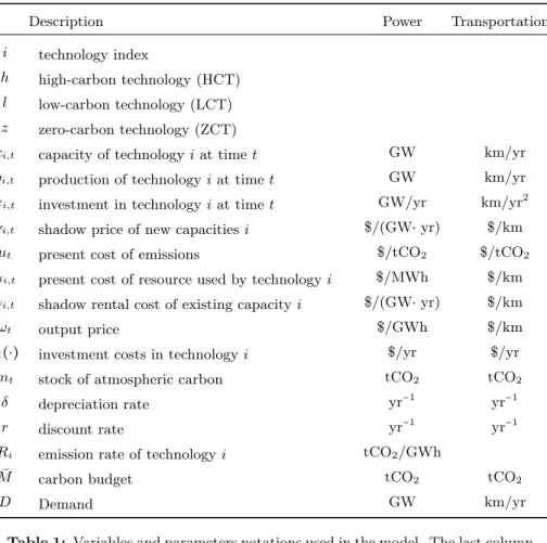
Notations are gathered in Table1.
Before presenting simplified and easy-to-understand first order conditions at the next subsection, we methodically write the Hamiltonian, full FOCs and complementary slackness conditions.8
The Hamiltonian reads: H =e−rt∑
i
ci(xi,t) − ∑
i
νi,t(xi,t−δ ki,t) +µt∑
i Riqi,t +ηt(mt− ¯M ) + ωt(D − ∑ i qi,t) + ∑ i
γi,t(qi,t−ki,t) − ∑ i λi,tqi,t− ∑ i ξi,txi,t− ∑ i λi,tqi,t− ∑ i ξi,txi,t + ∑ i αi,tqi,t− ∑ i βi,tSi,t (13)
7We end up with the same options thanCoulomb and Henriet(2013): our social planner may choose between a dirty backstop (e.g. coal), a clean backstop (renewable power), or a polluting exhaustible resource (gas).
8The transversality condition is replaced by the terminal condition that at some point the atmospheric carbon reaches its ceiling (6).
Description Power Transportation i technology index
h high-carbon technology (HCT) l low-carbon technology (LCT) z zero-carbon technology (ZCT)
ki,t capacity of technology i at time t GW km/yr
qi,t production of technology i at time t GW km/yr
xi,t investment in technology i at time t GW/yr km/yr2
νi,t shadow price of new capacities i $/(GW⋅ yr) $/km
µt present cost of emissions $/tCO2 $/tCO2
αi,t present cost of resource used by technology i $/MWh $/km
γi,t shadow rental cost of existing capacity i $/(GW⋅ yr) $/km
ωt output price $/GWh $/km
ci(⋅) investment costs in technology i $/yr $/yr
mt stock of atmospheric carbon tCO2 tCO2
δ depreciation rate yr−1 yr−1
r discount rate yr−1 yr−1
Ri emission rate of technology i tCO2/GWh
¯
M carbon budget tCO2 tCO2
D Demand GW km/yr
Table 1: Variables and parameters notations used in the model. The last column gives possible units for the electricity sector.
The first-order conditions are: ∂H
∂xi
=0 ⇐⇒ c′i(xi,t) =ert(νi,t+ξi,t) (14) ∂H
∂qi
=0 ⇐⇒ γi,t=λi,t−µtRi−αi,t+ωt (15)
˙ νi,t+
∂H ∂ki
=0 ⇐⇒ ν˙i,t−δνi,t=γi,t (16)
˙ µt+ ∂H ∂mt =0 ⇐⇒ µ˙t= −ηt (17) ˙ αi+ ∂H ∂Si =0 ⇐⇒ α˙i=βi,t (18)
The complementary slackness conditions are:
∀i, t, ξi,t≥0, xi,t≥0 and ξi,txi,t=0 (19) ∀i, t, λi,t≥0, qi,t≥0 and λi,tqi,t=0 (20) ∀i, t, ηt≥0, M − m¯ t≥0 and ηt ( ¯M − mt) =0 (21) ∀i, t, βi,t≥0, Si,t≥0 and βi,tSi,t=0 (22)
∀i, t, γi,t≥0, ki,t−qi,t≥0 and γi,t (ki,t−qi,t) =0 (23) ∀t, ωt≥0, D − ∑ i qi,t=0 and ωt(D − ∑ i qi,t) =0 (24)
3.2. Optimal costs when production and investment are positive
When production and investment are nonnegative, the multipliers associ-ated with their respective positivity constraints are nil (19,20), and first-order conditions (14,15,16) simplify to:
c′
i(xi,t) =ertνi,t (25)
˙
νi,t−δνi,t=ωt−µtRi−αi,t (26)
The simplified FOCs imply that when production and investment are non-negative, the optimal investment schedules xi,t satisfy the following differential
equation:9 (δ + r) c′ i(xi,t) − d dtc ′ i(xi,t) =ert (ωt−µtRi−αi,t) (27) The Left Hand Side term corresponds to whatVogt-Schilb et al.(2013) have called the implicit marginal rental cost of capital (MIRCC) pi,t:
pi,t= (δ + r) c′i(xi,t) − d dtc
′
i(xi,t) (28)
The MIRCC extends the concept of the implicit rental cost of capital proposed byJorgenson (1967) to the case of endogenous capacity prices. It corresponds to the efficient market rental price of capacities, where capitalists would be indifferent between (i) buy capital at t at a cost c′
i(xi,t), rent it out during one
period dt at a price pi,t, and sell the depreciated (δ) capacities at t + dt at a
price c′
i(xi,t) +dtdc′i(xi,t)dt or (ii) simply lend money at the interest rate r.
The RHS of (27) relates to the variable costs and revenues of a producer. The output is sold at its current price ertω
t(ωtinterprets as the output price,
as it is the shadow cost of the demand constraint (24)). Producing one unit of the output requires to use fuel bought at the current price αi,tert(see38below)
and pay for the emitted carbon Ri (5) at the current price µtert (see32).
Proposition 1. During a time interval (σi, τi)when production and investment are positive, the optimal marginal implicit rental cost of capital pi,t is equal to
the current price of the output ωtert minus the current cost of emissions µRiert
and minus the current price of fossil resources αiert.
pi,t=ert (ωt−µtRi−αi,t) (29) Prop. 1 can be seen as an application of the equimarginal principle. It provides a simple rule to arbitrate production decisions at each moment, by relating the output price, the rental cost of productive capacities and the variable costs. As the equimarginal principle applies to the decision of renting the capital, it does not directly describe trade-offs for investors. Investment decisions follow much more complex dynamics, studied in the remaining of this article.
9(25)−δd
dt(25) leads to e rt
(ν˙i,t−δνi,t) = (δ + r) c′i(xi,t) − d dtc
′
i(xi,t); substituting in (26) leads to the desired result.
Proposition 2. In an interval (σi, τi) when investment and production are positive, the optimal Marginal Investment Cost (MIC) can be expressed as a sum of two terms: (i) the present value of all future revenues from selling the output minus costs from emission and resource usage (ωθ−µRi−αi)produced by the depreciated marginal unit of capacity (e−δ(t−θ)), plus (ii) a term that tends to c′ i(xi,τi): ∀t ∈ (σi, τi), (30) c′ i(xi,t) =ert∫ τi t e−δ(t−θ)(ωθ−µθRi−αi,θ)dθ + e(r+δ)(t−τi)c′i(xi,τi)
Proof. Appendix Ashows that (30) is the textbook solution of (27).
Proposition 2 can be seen as a generalization of the previous finding by
Vogt-Schilb et al. (2012) that when abatement is obtained by accumulating low-carbon capital, optimal efforts to curb emissions are not necessarily growing over time.
Corollary 1. If investment in and usage of a technology i never stop after a date σi, the optimal MIC for that technology simply equals the present value
of all future revenues from selling the output minus costs from emission and resource usage produced by the depreciated marginal unit of capacity
∀t ∈ (σi, ∞), c′i(xi,t) =ert∫
∞
t
e−δ(t−θ)(ωθ−µθRi−αi,θ)dθ (31) Proof. Taking the limit of (30) when τi→ ∞leads to the result.10
Corollary 1 expresses the optimal investment cost of the technology used during the steady state (we show later that it is the zero-carbon technology).
Prop. 2 and Corollary 1 give a general relation between the optimal MIC and a discounted sum of future revenues during a time period when capacities are used (they do not provide more information than Prop. 1). Assessing the optimal investment costs in practice requires to express more concretely those net revenues, hence the output price ωt, the carbon price µt, the resource costs
αi,t, and the time period (σi, τi). Doing so is the purpose of the next section.
4. Transition phases, output price and explicit optimal investment costs
4.1. General phases
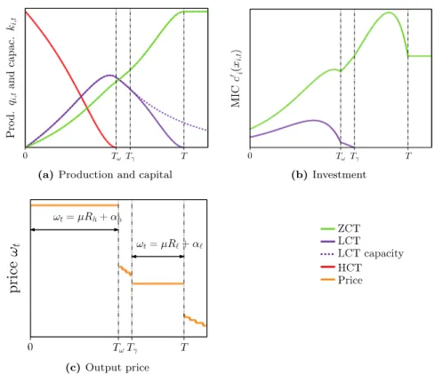
The number of inequalities combinations captured by the slackness condi-tions is large. The different cases may be tackled analytically if we assume that on the optimal path, the system passes through phases (this assumption is con-firmed by numerical simulations with standard functional forms, but cannot be proved for general functions). The following proposition and Fig.1 summarize our findings concerning those phases.
10 We implicitly made the (reasonable) assumption that c′
i(xi,t) is bounded if xi,t is bounded.
(a) Production and capital (b) Investment
(c) Output price
Figure 1: Illustration of the four main phases.
Proposition 3. The optimal pathway can be divided into four main phases: 1. In a first phase (for t ∈ [0, Tω]) HCT production decreases (compensated
by the increasing total production of LCT and ZCT) and the output price equals the (constant) emission costs plus the resource costs from the high-carbon technology: ωt=µRh+αh.
Then (for t ∈ [Tω, T ]) LCT production decreases and ZCT production
increases (LCT production may decrease before Tω).
2. In the second phase (t ∈ [Tω, Tγ]), LCT production decreases slower than
the natural rate of replacement of its capacity. Investment in LCT con-tinues even if its production decreases (x`,t<δk`,t).
3. In a third phase (for t ∈ [Tγ, T ]) LCT production decreases faster than
the natural depreciation rate of its capacity and the output price equals the sum of constant resource costs and constant emission costs from the low-carbon technology: ωt=µR`+α`.
4. At T , the system reaches a steady state, all production comes from the ZCT, emissions are nil, atmospheric pollution is at its ceiling. If low-carbon resources were binding they are exhausted at T (α`,TS`,T =0). In the remaining of this subsection we present four lemmas that build a proof for Prop.3.
Definition 1. Let Tair be the date when the ceiling on atmospheric carbon is
reached.
Before Tair, the social cost of carbon µtis constant (17,21):
∀t < Tair, µt=µ > 0 (32)
The carbon-free atmosphere can be seen as a non renewable resource depleted by GHG emissions. In this context, the optimal current carbon price µert follows the Hotelling’s rule, i.e. grows at the discount rate, as abatement realized at any time contributes equally to meet the carbon budget. The carbon price µ is strictly positive as we focus on the case where the carbon budget is binding. Definition 2. Let T be the date when the system reaches a steady state.
During the steady state, the ZCT produces all the output. Indeed, atmo-spheric carbon is stable, hence emissions from the ZCT and LCT must be nil (3,4):
∀t ≥ T, ˙mt=0 Ô⇒ q`,t=qh,t=0 (33) HCT production can stop before the system reaches a steady state.
Definition 3. Let Tω≤T be the date when high-carbon production stops.
∀t ≥ Tω, qh,t=0 (34)
Lemma 1. Before the HCT is phased out, the optimal output price ωtis equal
to the sum of variable cost and emission costs from the high-carbon technology:
∀t ≤ Tω, ωt=µRh+αh (35)
Proof. By assumption, the HCT capacity is always underused (qh,t<kh,t), hence
the multiplier associated with the capacity constraint is nil γh,t=0 (23). While h is used to produce the output, the multiplier associated with the positivity constraint is also nil λh,t =0 (20). The output price ωt can then be obtained
from (15).
In the power sector, Lemma1 means that while the marginal power plant is a coal power plant, the price of electricity is the cost of coal plus the carbon price times the emission rate of coal.
It is possible that at one point, production from the LCT declines. One possible reason is if fossil deposit are almost depleted. An other relates to GHG emissions. From the moment Tω, the demand constraint (4) makes it impossible
to reduce further emissions by using both additional ` and z. Total emissions can be reduced further by producing more with the ZCT and less with the LCT (since Rz<R`). Therefore, from Tω on, LCT production may decline to allow
for more ZCT production. In particular, it may become beneficial to use less ` than allowed by installed capacities.
Definition 4. Let Tγ ≤ min (TS`, Tair) be the date when LCT production is
lower than its capacity:
Lemma 2. Along the optimal path, when low-carbon capacities are used, but under full capacity, variable costs from LCT determine the output price:
∀t ∈ [Tγ, T ] ωt=µR`+α` (36)
Proof. The proof is similar to that of Lemma1.
Corollary 2. Along the optimal path, the low-carbon capacities may not be underused before high-carbon production is phased out.
Tγ>Tω
Proof. In general, the output price cannot be equal to the variable costs of both the HCT and the LCT (i.e. both Lemma 1 and Lemma 2 cannot hold at the same time). For instance, in the power sector, the marginal power plant may be coal or gas, but not both at the same time.11
Lemma 3. In the steady state, the output price equals the rental cost of the zero-carbon capacity:
∀t ≥ T ertωt=pz,t (37)
Proof. From Prop. 1, as the zero-carbon technology does not require to burn any resource (αz=0), nor pay for any emission (Rz=0).
In the power sector, Lemma3 means that when all the electricity is pro-duced from windmills, the market price of electricity equals the rental price of windmills.
Definition 5. Let TSi be the date when deposit i is depleted.
Fossil fuel prices follow the Hotelling rule, their present price αi,tis constant
before they are exhausted (18,22):
∀t < TSi, αi,t=αi>0 (38)
Lemma 4. Along the optimal path, if fossil resources are depleted before the steady state, they are exhausted the moment when atmospheric pollution reaches its ceiling and when the productive system reaches its steady state.
TSi≤T Ô⇒ TSi=Tair=T
If high-carbon are depleted before the steady state, then TSh=Tω
Proof. If low-carbon resources are eventually depleted, it happens at the date TS`. This date arrives after low-carbon capacity is underused, hence after the
HCT is phased out (TS` ≥Tγ ≥Tω) (Definition4 and Corollary2). Once
low-carbon resources are exhausted, all the demand must be satisfied by the zero carbon technology, hence the atmospheric carbon mt remains stable. As we
assumed the carbon budget is binding, ¯M is reached at this moment.
Concerning the high carbon resource: if they get depleted, this happens at TSh. At this moment, production from the HCT stops, hence TSh =Tω.
11We disregard the case where fuel costs compensate exactly differences in carbon intensities α`−αh=µ (Rh−R`)as it requires a very restrictive set of assumptions.
Lemma4and (38) ensure that fossil fuel prices αi,t are constant during the
whole time when the corresponding fossil fuels are used.
This subsection has provided insights on the general shape of the transition from high-carbon production to low-carbon and to zero-carbon production, and on the price of the output.We still lack a characterization of the period (σi, τi) during which the optimal marginal investment costs may be calculated explicitly (from Prop.2). The next subsection attempts to do so.
4.2. Sub-phases and ordering
Definition 6. Let Ti be the date when investment in capacity i starts. Let T`e
be the date when investment in the LCT ends.12
The HCT is phased out only after investment in one of the green technologies started:
Tω≥min(T`, Tz) (39)
If the low-carbon capacity is underused, investment in new low-carbon capacity is not optimal. Therefore the latter stops before LCT production drops below installed capacity:
T`e≤Tγ (40)
Lemma 5. ZCT investment starts before LCT investment ends (Tz≤T`e) Proof. At any given time, existing capacities are used in the merit order, i.e. capacities with the lowest variable cost are used first. This means that LCT production is never replaced by HCT production (9), or in other terms total instantaneous emissions never increase.
If LCT investment stops before investment in the ZCT starts, i.e. before ZCT production starts replacing HCT and LCT production, LCT production necessarily decreases at least with the depreciation rate of LCT capacity, and hence is replaced by HCT production to comply with the demand constraint, which is in contradicion with the previous statement.
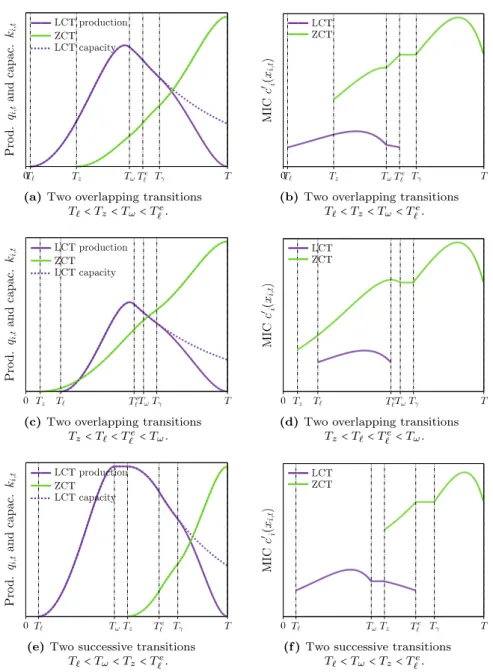
Several ordering possibilities remain, summarized in the following proposi-tion:
Proposition 4. Investment phases may be ordered in following ways (Fig.2): 1. Two successive transitions, starting with LCT investment. The LCT com-pletely replaces the HCT first, then the ZCT replaces the LCT (Fig. 2e). 2. Two overlapping transitions, with a phase of simultaneous investment in the LCT and the ZCT. Investment in the LCT start first, and invest-ment in the ZCT start before the HCT has been completely replaced (Fig.
2a). Investment in the LCT can stop before or after the HCT has been completely replaced.
12 We do not need an equivalent definition for the ZCT as it used in the steady state and investment never stop.
(a) Two overlapping transitions T`<Tz<Tω<T`e.
(b) Two overlapping transitions T`<Tz<Tω<T`e.
(c) Two overlapping transitions Tz<T`<T`e<Tω.
(d) Two overlapping transitions Tz<T`<T`e<Tω.
(e) Two successive transitions T`<Tω<Tz<T`e.
(f ) Two successive transitions T`<Tω<Tz<T`e.
Figure 2: Numerical simulations displaying three possible transition profiles. Figures on the left display capacities and productions, figures on the right display optimal MICs. Appendix B describes the parameters used to produce these figures (assumption (10) holds in every simulation).
3. Two overlapping transitions, with a phase of simultaneous investment in the LCT and the ZCT. Investment in the more expensive ZCT start first, and investment in the LCT start before the HCT has been completely re-placed. Investment in the LCT can stop before or after the HCT has been completely replaced (Fig. 2c).
Prop.4 is similar to the finding byChakravorty et al. (2008) that the op-timal extraction of several polluting nonrenewable resources may follow several unintuitive orderings. In their work, however, the dynamics comes from the interaction of several scarcity rents; in ours, it comes from the convexity on investment costs.
4.3. Explicit optimal marginal investment costs
Using previous results, the optimal MIC for the LCT and the ZCT can be expressed as a function of the carbon price and the resource costs during the different phases, refining the general expression given by Eq.30:
∀t ≥ Tz, e−rtc′z(xz,t) = ∫ Tω t e−δ(t−θ)(µ Rh+αh)dθ +∫ Tγ Tω e−δ(t−θ)ωθdθ + ∫ T Tγ e−δ(t−θ)(µ Rl+α`)dθ +∫ ∞ T e−δ(t−θ)ωθdθ ∀t ∈ [T`, T`e], e −rt c′ `(x`,t) = ∫ Tω t e−δ(t−θ)(µ (Rh−R`) +αh−α`)dθ (41) + ∫ T`e Tω e−δ(t−θ)(ωθ−µ R`−α`)dθ + c′`(0) e (r+δ)(t−Te `)
Proposition 5. When the social planner invests in both the ZCT and the LCT, it builds zero-carbon capacity at a higher cost than low-carbon capacity.
Proof. From (41): ∀t ∈ [max i (Ti), T e `], c ′ z(xz,t) −c′`(x`,t) = (µ R`+α`)ert∫ Te ` t e−δ(θ−t)dθ ´¹¹¹¹¹¹¹¹¹¹¹¹¹¹¹¹¹¹¹¹¹¹¹¹¹¹¹¹¹¹¹¹¹¹¹¹¹¹¹¹¹¹¹¹¹¹¹¹¹¹¹¹¹¹¹¹¹¹¹¹¹¹¹¹¹¹¹¹¹¹¹¹¹¹¹¹¹¹¹¹¹¹¹¹¹¹¹¹¹¹¹¹¹¹¹¹¹¹¸¹¹¹¹¹¹¹¹¹¹¹¹¹¹¹¹¹¹¹¹¹¹¹¹¹¹¹¹¹¹¹¹¹¹¹¹¹¹¹¹¹¹¹¹¹¹¹¹¹¹¹¹¹¹¹¹¹¹¹¹¹¹¹¹¹¹¹¹¹¹¹¹¹¹¹¹¹¹¹¹¹¹¹¹¹¹¹¹¹¹¹¹¹¹¹¹¹¹¶ ∆p + (c′ z(xz,Te `) −c ′ `(0)) e (r+δ)(t−T`e) ´¹¹¹¹¹¹¹¹¹¹¹¹¹¹¹¹¹¹¹¹¹¹¹¹¹¹¹¹¹¹¹¹¹¹¹¹¹¹¹¹¹¹¹¹¹¹¹¹¹¹¹¹¹¹¹¹¹¹¹¹¹¹¹¹¹¹¹¹¹¹¹¹¹¹¹¹¹¹¹¹¹¹¹¹¹¹¹¹¹¹¹¹¹¹¹¹¹¹¹¹¸¹¹¹¹¹¹¹¹¹¹¹¹¹¹¹¹¹¹¹¹¹¹¹¹¹¹¹¹¹¹¹¹¹¹¹¹¹¹¹¹¹¹¹¹¹¹¹¹¹¹¹¹¹¹¹¹¹¹¹¹¹¹¹¹¹¹¹¹¹¹¹¹¹¹¹¹¹¹¹¹¹¹¹¹¹¹¹¹¹¹¹¹¹¹¹¹¹¹¹¶ ∆c′ (42)
∆p is the discounted value of emissions and fossil fuels that the marginal zero-carbon capacity built at time t allows to save before T`ewhen compared to the marginal low-carbon capacity built at time t.
∆c′ is the difference between the values of the marginal capacities built at Te `
discounted to t. It is strictly positive, as c′ z(xz,Te `) >c ′ z(0) as c ′ z is growing by assumption and c′ z(0) > c′`(0) (10).
The left column of Fig.2 illustrates Prop.5. In particular, Fig.2fdisplays a case where it is optimal to start with the most expensive option, similarly to the previous result byVogt-Schilb and Hallegatte(2011).
While more accurate than (30), Eq. 41does not give a direct assessment of the optimal investment cost in any of the two technologies. In particular, the output price when the LCT is fully used and during the steady state is unknown (ωt, t ∈ [Tω, Tγ] ∪ [T, ∞)), as well as the amount of investment in the ZCT
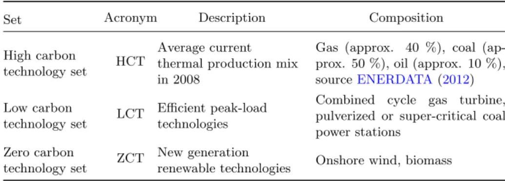
Table 2: Technology sets considered in the numerical model
Set Acronym Description Composition
High carbon
technology set HCT
Average current thermal production mix in 2008
Gas (approx. 40 %), coal (ap-prox. 50 %), oil (ap(ap-prox. 10 %), sourceENERDATA(2012) Low carbon
technology set LCT
Efficient peak-load technologies
Combined cycle gas turbine, pulverized or super-critical coal power stations
Zero carbon
technology set ZCT
New generation
renewable technologies Onshore wind, biomass
when investment in the LCT stops (c′ z(xz,Te
`)), and the dates when the different
phases begin and end.
In order to investigate whether the levelized cost of low-carbon capital can provide an accurate rule of thumb to assess investment in different types of low-carbon capital, the next section uses a numerical version of the model calibrated on the European electricity sector.
5. Numerical application: the case of the European electricity sector 5.1. Modeling framework, data, calibration
Let us calibrate a modified version of our model with data from the European power sector. In this numerical application, efficient gas power plants (the LCT) and renewable power (the ZCT) are used to phase out the existing emitting capacities represented as the average current thermal production mix. Table2
gives the aggregation of technology sets used in the numerical simulation. To better fit the data, we express installed capacity ki,t in peak capacity
(GW), and production qi,t in GWh/yr. Production is then constrained by a
maximum number of operating hours Hi(lower for renewables to capture
inter-mittency issues). We then define the utilization rate ui,t of installed technology
i at time t as:
ui,t= qi,t
Hiki,t
(43) We also model different lifetimes for different technologies, hence different de-preciation rates δi (renewable plants have shorter lifetimes than fossil-fueled
plants).
As resource depletion happens at the global scale, we consider that Europe is price-taker for exhaustible resources (coal and gas), which costs are included in the form of fuel costs αi (constant in present value).
The model becomes (omitting the positivity constraints): min
xi,t,qi,t∫
∞
0 ∑i
(e−r tci(xi,t) +αiqi,t)dt (44)
s.t. ˙ki,t=xi,t−δiki,t
Table 3: Technology-specific data used in the numerical application.
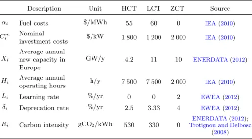
Description Unit HCT LCT ZCT Source
αi Fuel costs $/MWh 55 60 0 IEA(2010)
Cim Nominal
investment costs $/kW 1 800 1 200 2 000 IEA(2010)
Xi Average annual new capacity in Europe GW/y 4.2 11 10 ENERDATA(2012) Hi Average annual
operating hours h/y 7 500 7 500 2 000 IEA(2010)
Li Learning rate %/yr 0 0 2 EWEA(2012)
δi Deprecation rate %/yr 2.5 3.33 4 EWEA(2012)
Ri Carbon intensity gCO2/kWh 530 330 0
ENERDATA(2012);
Trotignon and Delbosc (2008)
Table 4: General parameter values used in the numerical application.
Description Unit Value Source
r Discount rate %/y 5
¯
M Carbon budget GtCO2 17 UE(2011);Trotignon
and Delbosc(2008)
D Power demand TWh/y 1 940 ENERDATA(2012)
A Convexity parameter ⋅ 0.1 ∑ i qi,t=D ˙ mt= ∑ i Riqi,t mt≤M¯
We assume quadratic investment costs. To add some realism, we complete the cost function with an exogenous learning rate Li.13 To calibrate the cost
functions, we assume that when investment equals the average annual invest-ment flow in Europe between 2009 and 2011 (Xi), the marginal investment cost
Cimis equal to the OECD median value for 2010 (as found inIEA(2010)). We write the cost function as:
ci(xi,t) =Cim⋅Xi⋅ (A xi,t Xi + 1 − A 2 ( xi,t Xi ) 2 ) ⋅e−Lit (45) t = 0 Ô⇒ c′ i(Xi) =Cim (46)
13The numerical simulations show that adding this feature does not change the qualitative form of the solution: the transition still displays the phases described in the analytical section.
A is a convexity parameter, assumed equal across technologies. If A = 1, the marginal investment cost is constant (the cost of new capacity does not depend on the investment pace), and optimal investment pathways would exhibit jumps: there would be no economic inertia (Vogt-Schilb et al., 2012). If A = 0 the marginal cost curves become linear (the cost of new capacity doubles when the investment pace doubles) and capacity accumulated at very low speed is almost free (limxi,t→0;A=0 c
′
i(xi,t) = 0). An intermediate value A ∈ (0, 1) means that new capacity is always costly, and that its cost grows with the investment pace. The illustrations in this section are obtained with A = 0.1, i.e. with a relativeley low convexity (investment cost doubles at 2.11 times the nominal pace).
The emission allowances allocated to the power sector amounted to Eref = 1.03 GtCO2/yr in 2008 (Trotignon and Delbosc, 2008). The reference fossil
energy production (from coal, oil and gas) was D = 1 940 TWh/yr that year (ENERDATA, 2012), leading to a reference emission rate of 530 tCO2/GWh.
We take a carbon budget corresponding to roughly half of the BAU cumulative emissions, i.e. 17 GtCO2.
We calibrate the depreciation rate as δi =1/lifetime and assume a lifetime of 30 years for the existing capacity and new gas and 25 years for wind (IEA,
2010). We use r = 5 %/yr for the social discount rate. 5.2. Results
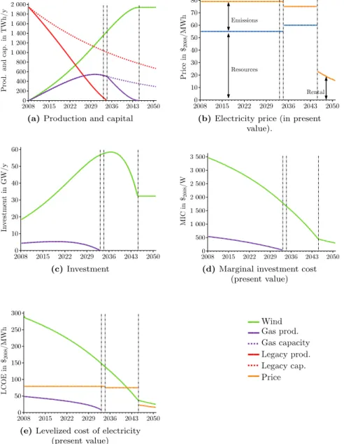
Fig.3shows various variables of the numerical application to the European electricity sector. First of all, the investment profile goes through the phases discussed in the theoretical section. Results from Section 4 are robust to the particular extensions made in this section (the social planner can invest in dirty capital, depreciation rates are different for wind, gas and legacy capacity, there is exogenous learning for wind). In particular, the social planner does not invest in the legacy capacity, which is entirely phased out in 2035 (Fig.3a). There is unused gas capacity as soon as the dirty technology is phased out (Tγ =Tω = 2035), and investment in gas stops a couple of years earlier (T`e=2033).
Investment in both efficient gas and renewable power starts from the be-ginning of the simulation (Fig. 3c). The exogenous technical progress on the windmills is not sufficient to postpone investment in windmills in the optimal solution. Until 2038, investment in windmills grows over time. Investment starts at 18 GW/yr in 2008, almost twice the actual average investment rate Xi, and
reach 60 GW/yr in 2038. It decreases after 2040 as most of the power plants have already been replaced (Fig.3a), and stay constant after 2045 to maintain the wind capacity constant.
Fig.3ddisplays the resulting marginal costs for new capacity (MICs) along the period, expressed in present value. They decrease over time, as the average power plants becomes less and less carbon-intensive, making investment in low carbon capacity less and less profitable. Investment in gas remains relatively low by contrast. Prop. 5 holds: the MIC is always higher for the renewables, despite renewable being subject to exogenous technical progress and having a higher depreciation rate (both reasons to invest less in renewables in the short term).
Electricity prices are displayed in Fig.3b. While production comes from fos-sil resources the price decomposes as resource cost and emission cost (Lemma1
(a) Production and capital (b) Electricity price (in present value).
(c) Investment (d) Marginal investment cost (present value)
(e) Levelized cost of electricity (present value)
Figure 3: Outputs from the numerical application to the European electricity sector
dirty technology, and the electricity price is high. After the dirty technology has been phased out, from 2035 to 2045, gas becomes the marginal technology and the price drops. The endogenous carbon price is 46$/tCO2, and the lower
carbon intensity of gas compared to coal more than compensates the higher resource cost. In the last phase, all the electricity comes from renewable power, and electricity price equals the rental cost of renewable power plants (Lemma3). This rental cost decreases because we assumed exogenous technical progress in the renewable power sector (see Li in equation B.1and Table3).
5.3. Levelized Cost Of Electricity
Levelized costs of electricity are frequently used to compare different tech-nologies in the power sector, sometimes with the underlying idea that technolo-gies with lower LCOEs are cheaper, hence superior, to technolotechnolo-gies with higher LCOEs (e.g.IPCC,2007; Alok,2011;Kost et al., 2012; EIA,2013).
As the cost-efficiency of investment in low-carbon capital is not easy to assess precisely (Section4.3), a question is whether the LCOE may be used as a good proxy.
Definition 7. The Levelized Cost of Electricity (LCOE), denoted Li,t, is the
ratio of discounted costs to discounted production of the marginal capacity (we express them in present value):
Li,t= e−rtc′
i(xi,t) + ∫t∞(µRi+αi,θ)ui,θe−δi(θ−t)dθ
∫
∞
t ui,θ e−(r+δi)(θ−t)dθ
(47)
The total costs from the marginal capacity built at t express as the in-vestment cost c′
i(xi,t), plus the variable costs (µRi+αi,θ)associated with the marginal capacity along its lifetime (during which it will depreciate at the rate δi and will be used at a rate ui,θ (43)). The denominator is the discounted
production of the depreciating marginal unit of capacity over time.
Fig. 3e shows the levelized costs of electricity along the optimal pathway simulated for the European Union, and compare them with the corresponding electricity price. Optimal LCOEs differ among technologies, and differ from the electricity price. The optimal LCOEs of wind are found higher than electricity prices, and electricity prices are themselves higher than the LCOE generated from gas.
Indeed, investment costs should be higher in renewable power for three rea-sons (i) renewable power saves more GHG than gas, (ii) renewable power saves fossil energy, compared to gas, and (iii) renewable power is more useful than gas in the long term. Levelized cost of electricity account for fixed investment costs, GHG emissions and variable energy costs, but they leave aside the third reason (in other terms, they “forget” the ∆c′ term from Prop.5). This term accounts
for the fact that renewable power will be used forever (during the steady state), while at some point investment in gas power must stop as gas plants built to phase the coal out shall themselves be eventually replaced by renewable power.
Vogt-Schilb et al. (2013) demonstrate that a similar criteria (the levelized abatement cost) is accurate only if capacity costs are constant in time and do not depend on the investment pace. In our numerical simulations, even if the capacity cost slowly increases with the investment pace (the convexity of the cost function is low A = 0.1), the optimal levelized cost of electricity produced
from renewable sources is almost six times greater than the levelized cost of electricity produced from gas. This suggests that LCOEs should not be used as a rule-of-thumb metrics to assess investment.14
In our simulation, if decision makers decided investment in new capacity by comparing LCOEs to electricity price, they would build too much low-carbon capacity, and not enough zero-carbon capacity.
6. Conclusion
We investigate in an analytical model the optimal timing of investment in low-carbon (e.g. gas power plant, efficient thermal vehicles) and zero-carbon (e.g. renewable power, electric vehicles) capital to phase out preexisting high-carbon capital within a sector facing an inelastic demand (electricity or private mobility) and a carbon budget. We then run numerical simulations calibrated on the European power sector.
We find that in a first phase, new gas and renewable power plants should progressively replace the preexisting higher-carbon plants. During this phase, the electricity price equals the variable costs of producing electricity from coal (i.e. energy costs and the cost of carbon emissions). Then, electricity is produced by both types of greener capital used at full capacity. The renewable power plants continue to accumulate to increase current abatement, and the social planner allows the natural depreciation process to decrease available gas power capacities. In a third period, gas power plants may be underused, to allow even more abatement to be performed by production from additional renewable power plants. In this period, the market price of electricity equals the cost of buying gas and paying for induced GHG emissions. Finally, a steady state is reached where all the production comes from renewable carbon-free power.15
Within our modeling framework, the availability of gas resources does not modify qualitatively these phases. This finding contrasts with previous re-sults from the resource economics literature. Further research could investigate whether it comes from assumptions made for analytical simplification (namely constant demand and no proportional natural dilution of atmospheric pollu-tion) or from assumptions made for realism (consuming resources requires to accumulate adequate capital at a convex cost).
Another finding is that the ordering of investment does not follow any eas-ily predetermined order; in particular, investment in the expensive carbon-free capital (renewable power, electric vehicles) may begin at the same time, or even before, investment in the lower-cost low-carbon capital (e.g gas plants, efficient thermal engines).
Assessing the optimal cost of investment in low-carbon capital turns out to be tricky. In our model, the equimarginal principle gives information on the optimal price at which capacities should be rented once constructed. In the power sector, for instance, this results in equalizing the rental cost of a particular plant plus the costs of buying fuel and paying for the GHG emissions to the price of electricity. It does not give a direct information on the social cost at which new capacities
14 Further research should carry out a sensitivity analysis on the convexity parameter A and the climate policy stringency ¯M .
should be built in the first place. In theory, the optimal investment cost simply expresses as the discounted sum of all future revenues derived from renting the capital (Section 3.2). However, actually calculating optimal investment costs requires to solve the model backward, and in particular to know in advance the output price along the various investment and production phases.
The only analytical result concerning optimal investment costs is that, when capacities in both gas and renewable power are being built, we should always invests more dollars per installed capacity in renewable power. This is not explained only by cheaper operation costs of renewable power coming from both the carbon price and nil fossil energy requirements. Renewable power may be used forever, while the exhaustible and polluting low-carbon capacity built to phase out the preexisting dirtier plants will eventually be phased out itself by the renewable power. The same conclusion applies in the private transportation sector: if electric vehicles and efficient thermal vehicles are built at the same time, electric vehicles should be built at a higher cost.
In practice, a tempting approach to assess the optimal cost of investment in low- and zero-carbon capital could be to use a rule based on the levelized cost. The investment criteria would be to build new capacities that appear competitive, e.g. would produce electricity at a levelized costs lower or equal to the market price (a hasty equimarginal principle). In our numerical simulations, along the optimal path, the levelized cost of electricity produced from renewable sources is almost six times greater than the levelized cost of electricity produced from gas. This suggests that ranking technologies according to their levelized cost of electricity would lead to too much investment in intermediate technolo-gies (such as gas or efficient thermal vehicles), and too little in more expensive zero-carbon capital (as renewable power or electric vehicles). The levelized cost does not provide enough information to assess and rank investment in polluting fossil-fueled and zero-carbon capital.
Acknowledgments
We thank St´ephane Hallegatte, Guy Meunier, Antonin Pottier, Philippe Quirion and Julie Rozenberg for useful comments and suggestions. We are grateful to Patrice Dumas for technical support. This work benefit from finan-cial support from the Institut pour la Mobilit´e Durable, from ´Ecole des Ponts ParisTech.
References References
Acemoglu, D., Aghion, P., Bursztyn, L., Hemous, D., 2012. The environment and directed technical change. American Economic Review 102 (1), 131–166. Allen, M., Frame, D., Huntingford, C., Jones, C., Lowe, J., Meinshausen, M., Meinshausen, N., 2009. Warming caused by cumulative carbon emissions to-wards the trillionth tonne. Nature 458 (7242), 1163–1166.
Chakravorty, U., Moreaux, M., Tidball, M., 2008. Ordering the extraction of polluting nonrenewable resources. The American Economic Review 98 (3), pp. 1128–1144.
Coulomb, R., Henriet, F., 2013. The Grey Paradox: How Oil Owners Can Benefit From Carbon Regulation. PSE Working Paper 2013-11.
Delucchi, M. A., Lipman, T. E., 2001. An analysis of the retail and lifecycle cost of battery-powered electric vehicles. Transportation Research Part D: Transport and Environment 6 (6), 371–404.
DOE, 2013. EV everywhere grand challenge blueprint. Tech. rep., U.S. Depart-ment of Energy.
EIA, 2013. Levelized cost of new generation resources in the annual energy outlook 2013. Tech. rep., Energy Information Administration.
ENERDATA, 2012. Global energy & CO2database. Consulted May 2012.
EWEA, 2012. Wind in power: 2011 european statistics. Tech. rep.
Fischer, C., Newell, R. G., 2008. Environmental and technology policies for climate mitigation. Journal of Environmental Economics and Management 55, 142–162.
Fischer, C., Withagen, C., Toman, M., 2004. Optimal investment in clean pro-duction capacity. Environmental and Resource Economics 28 (3), 325–345. Gerlagh, R., Kverndokk, S., Rosendahl, K. E., 2009. Optimal timing of climate
change policy: Interaction between carbon taxes and innovation externalities. Environmental and Resource Economics 43 (3), 369–390.
Goulder, L., Mathai, K., 2000. Optimal co2abatement in the presence of induced
technological change. Journal of Environmental Economics and Management 39 (1), 1–38.
Herfindahl, O. C., 1967. Depletion and economic theory. Extractive resources and taxation, 63–90.
IEA, 2010. Projected cost of generating electricity, 2010 edition. Tech. rep., International Energy Agency.
IPCC, 2007. Cost analyses. In: Fourth Assessment Report.
Jorgenson, D., 1967. The theory of investment behavior. In: Determinants of investment behavior. NBER, pp. 129–188.
Kost, C., Jessica Thomsen, Sebastian Nold, Johannes Mayer, 2012. Levelized cost of electricity renewable energies. Tech. rep., Fraunhofer ISE.
Matthews, H., Gillett, N., Stott, P., Zickfeld, K., 2009. The proportionality of global warming to cumulative carbon emissions. Nature 459 (7248), 829–832. Ogden, J. M., Williams, R. H., Larson, E. D., 2004. Societal lifecycle costs of
Ploeg, F., Withagen, C., 1991. Pollution control and the ramsey problem. En-vironmental & Resource Economics 1 (2), 215–236.
Rozenberg, J., Vogt-Schilb, A., Hallegatte, S., 2013. Incentives in favor of green capital and intertemporal distribution of abatement efforts. Cired Working Paper.
Trotignon, R., Delbosc, A., 2008. Echanges de quotas en periode d’essai du marche europeen du CO2 : ce que revele le CITL. Etude climat 13, Caisse
des d´epots, Mission climat.
UE, 2011. A roadmap for moving to a competitive low carbon economy in 2050. Communication from the Commission COM(2011) 112 final, European Com-mission.
Vogt-Schilb, A., Hallegatte, S., 2011. When starting with the most expensive option makes sense: Use and misuse of marginal abatement cost curves. Policy Research Working Paper 5803, World Bank.
Vogt-Schilb, A., Meunier, G., Hallegatte, S., 2012. How inertia and limited potentials affect the timing of sectoral abatements in optimal climate policy. World Bank Policy Research (6154).
Vogt-Schilb, A., Meunier, G., Hallegatte, S., 2013. Should marginal abatement costs be different across sectors? The effect of green capital accumulation. World Bank Policy Research (6415).
Wikibooks contributors, 2013. First order linear 1. In: Ordinary Differential Equations. Wikibooks.
URL http://en.wikibooks.org/w/index.php?title=Ordinary_ Differential_Equations/First_Order_Linear_1&oldid=2486909
Appendix A. Solving for optimal MICs (proof of proposition 2) We use the generic algorithm to solve the following first-order linear differ-ential equation:
d dtc
′
i(xi,t) = (δ + r) c′i(xi,t) −ert (ωt−µ Ri−αi ) (A.1)
The general theory16 ensures that if zi,t satisfies:
˙
zi,t= −e−(δ+r)t (ert(ωt−µ Ri−αi )) (A.2) Then c′
i(xi,t) =e(δ+r)tzi,t is a solution of (A.1). The general solution of (A.2)
on an interval (σi, τi)reads: zi,t=zi,τi+ ∫
τi
t
e−(δ+r)θerθ(ωθ−µ Ri−αi )dθ (A.3)
Leading to: c′ i(xi,t) =e(δ+r)tzi,τi+e (δ+r)t ∫ τi t e−(δ+r)θerθ(ωθ−µ Ri−αi )dθ (A.4) =e(δ+r)tzi,τi+e rt ∫ τi t e −δ(t−θ) (ωθ−µ Ri−αi)dθ (A.5)
The constant zi,τi may be determined by evaluating the RHS at t = τi, leading
to: c′ i(xi,t) =e(r+δ)(t−τi)c′i(xi,τi) +e rt ∫ τi t e−δ(t−θ)(ωθ−µ Ri−αi)dθ (A.6)
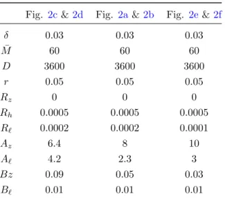
Appendix B. Numerical values used to produce Fig. 2
The simulations displayed in Fig.2were produced using the following quadratic cost functions, and parameters described in Table B.5:
ci(xi,t) =Aixi,t+Bi 2 x
2
i,t (B.1)
Fig. 2c&2d Fig. 2a&2b Fig. 2e&2f
δ 0.03 0.03 0.03 ¯ M 60 60 60 D 3600 3600 3600 r 0.05 0.05 0.05 Rz 0 0 0 Rh 0.0005 0.0005 0.0005 R` 0.0002 0.0002 0.0001 Az 6.4 8 10 A` 4.2 2.3 3 Bz 0.09 0.05 0.03 B` 0.01 0.01 0.01