Thermal performance study of foundation walls insulated with low emissivity material and furred airspace

Publisher’s version / Version de l'éditeur:

Vous avez des questions? Nous pouvons vous aider. Pour communiquer directement avec un auteur, consultez la

première page de la revue dans laquelle son article a été publié afin de trouver ses coordonnées. Si vous n’arrivez pas à les repérer, communiquez avec nous à PublicationsArchive-ArchivesPublications@nrc-cnrc.gc.ca.

Questions? Contact the NRC Publications Archive team at

PublicationsArchive-ArchivesPublications@nrc-cnrc.gc.ca. If you wish to email the authors directly, please see the first page of the publication for their contact information.

https://publications-cnrc.canada.ca/fra/droits

L’accès à ce site Web et l’utilisation de son contenu sont assujettis aux conditions présentées dans le site LISEZ CES CONDITIONS ATTENTIVEMENT AVANT D’UTILISER CE SITE WEB.

Internal Report (National Research Council of Canada. Institute for Research in Construction), 2005-04-25

READ THESE TERMS AND CONDITIONS CAREFULLY BEFORE USING THIS WEBSITE. https://nrc-publications.canada.ca/eng/copyright

NRC Publications Archive Record / Notice des Archives des publications du CNRC :

https://nrc-publications.canada.ca/eng/view/object/?id=1f2b1ec9-c45b-43f9-8589-f25d62b6854a https://publications-cnrc.canada.ca/fra/voir/objet/?id=1f2b1ec9-c45b-43f9-8589-f25d62b6854a

NRC Publications Archive

Archives des publications du CNRC

For the publisher’s version, please access the DOI link below./ Pour consulter la version de l’éditeur, utilisez le lien DOI ci-dessous.

https://doi.org/10.4224/20377818

Access and use of this website and the material on it are subject to the Terms and Conditions set forth at Thermal performance study of foundation walls insulated with low emissivity material and furred airspace

Natlonal Research Council Consell natlonal de recherches

1&1

lnstltule for lnstitut de

Research in Construction recherche en construction Ottawa Canada

K1 A OR6

Internal Report

Thermal Performance Study of Foundation Walls

Insulated with Low Emissivity Material and Furred

Airspace.

Submitted to

CCMC

Institute for Research in Construction

Thermal Performance Study of Foundation Walls Insulated

with Low Emissivity Material and Furred Airspace.

Authors:

Quality Assurance:

Group Leader :

Approved

:

Director, Building Envelope & Structure Program

Report No: Isofoill(1) Report Date: 25 April 2005 Contract No: None

Reference: None

Program: Building Envelope and Structure

30 pages Copy No. 1 of 1 copies

I.

Introduction

The client, CCMC, requested that BE&S provide technical and experimental input toward a technical guide that CCMC is preparing. The CCMC guide is titled "Foundation Wall Systems with Low Emissivity Sheet Material and

Furred-Airspaces Assembly". Specifically BE&S through this report, will provide the required thermal and material evaluation procedures for a low emissivity surfaced expanded polystyrene insulation sheet. In terms of thermal performance, the product would be evaluated as both a material and as a thermallly resistant component within a furred airspace insulated basement wall system.

2.

Objective

The main objective of this report is to provide, through standard experimental procedures supported by calculated technical data, the specific evaluation methods

& procedure to be followed in the proposed technical guide.

3.

Material Evaluation

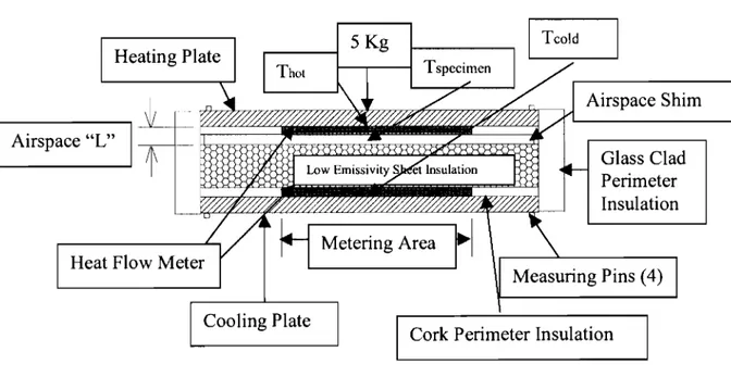
The thermal resistance and surface emissivity of the Low Emissivity Sheet Material should be determined by testing the Low Emissivity Sheet Material in

combination with air spaces of 0 mm, 3 mm, 6 mm and 9 mm in a Heat Flow Meter

Apparatus (Figure 1.0). The thermal resistance of the insulation (and in combination with the air spaces) should be determined in accordance with ASTM C 177 or ASTM C 518.

3.1 Specimen Measurements

Before setting up for testing in the Heat Flow Apparatus, the following measurements should be camed out and recorded on the low emissivity board insulation specimen.

3.1.1 Thickness A thickness gauge should be used to measure the thickness of at 17 randomly spaced points marked on one of the specimen's surface. The thickness is the average of these 17 measured points (mm).

3.1.2 Mass -The mass of the specimen should be recorded (grams).

3.1.3 Area

-

3.1.4 Volume

-

3.1.5 Density

-

3.2 Heat Flow Meter Specimen Set Up 3.2.1 Specimen Placement

A brush should be used in order to remove any dust or debris from the contact areas of the heating and cooling plates.

The specimen should be centered on the cooling plate (lower plate) the heating plate should then be placed (upper plate) on the specimen, insuring that the specimen remains centered over the heating and cooling plates (see Figure 1.0). If the specimen does not cover the plates, a material of similar conductivity and thickness should be used as a mask to completely cover the plates.

For the emissivity testing, air space plate spacers should be utilized. They should be placed between the heating plate and cooling plate at the comers of the apparatus. Small pine pieces of 3 mm thickness and of identical heights should be used for the respective tests of 3,6,9 mm airspaces.

3.2.2 Edge insulation

Twenty-five mm thick strips of edge insulation (glass clad) should be placed around the perimeter of the test specimen. The edge insulation should be cut such that it fits tightly between the cooling and heating plates.

3.2.3 Uniform Contact

To ensure an even contact between the heating/cooling plates and the test specimen, the apparatus should be placed between ring clamps (at least one on each side of the apparatus) or place weights of at least 5 Kg. on top of the apparatus

3.2.4 Thickness Measurement

Using a vernier, the thickness of the heating/cooling plates, plus the test specimen at the four outside comer measuring pins of the HFM should be measured.

The specimen thickness should be calculated by means of the following equation:

Where,

L = Specimen thickness

I,

I,,,

n = number of the outer comers (1,2, 3, or 4)

3.3 Heat Flow Apparatus Guard Placement

The entire test apparatus should be covered with an insulated cabinet or environment box. During the entire test maintain the ambient temperature at the

mean temperature (T,) by heating or cooling the enclosed environment. If no T, is

specified, use the setting indicated in Table 1.

Cork Perimeter Insulation

3.4Test Procedure

3.4.1 Temperature Settings

The heating and cooling units of the eat Flow Apparatus should be set to the standard test conditions as presented in Table 1 .O.

Table 1 .O: Standard Test Conditions

3.4.2 Test Steady-State (Thermal Equilibrium)

Variable

Hot Plate Temperature (Th) Cold Plate Temperature (Tc) Mean Temperature (T,) Temperature Difference (AT)

A thermal steady-state condition is achieved when:

The heat flow meter outputs from the hot and cold sides are in equilibrium The mean temperature is stable

The hot surface temperature and the cold surface temperature are stable The thermal steady-state conditions are maintained for a minimum of 12 hours.

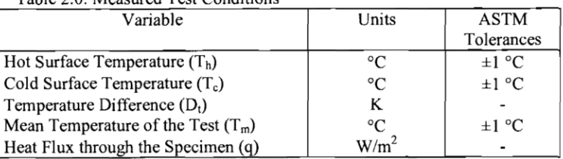
Table 2.0: Measured Test Conditions

Variable Units ASTM

1

Temperature ("C) 35.0 13.0 24.0 22.0 Measurement Tolerance ("C)

+

+

Hot Surface Temperature (Th) Cold Surface Temperature (Tc) Temperature Difference (D,) Mean Temperature of the Test (T,) Heat Flux through the Specimen (q)

"

-

3.5 Reporting

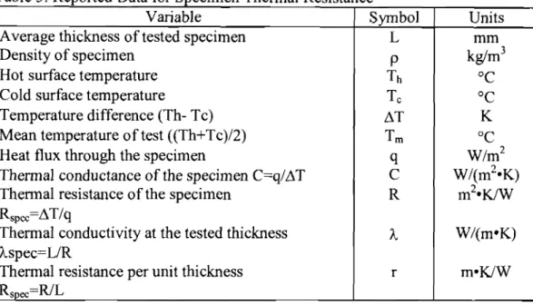
3.5.1 Thermal Resistance of Low Emissivity Sheet Material

The following collected and calculated data should be provided in the test

report. For the test with no airspace in place (0 mm), where the thermal resistance

of the material itself is measured the data provided should be as outlined in Table 3.

Table 3: Reported Data for Specimen Thermal Resista

Variable Average thickness of tested specimen Density of specimen

Hot surface temperature Cold surface temperature

Temperature difference (Th- Tc) Mean temperature of test ((Th+Tc)/2) Heat flux through the specimen

Thermal conductance of the specimen C=q/AT Thermal resistance of the specimen

R,,,=AT/q

Thermal conductivity at the tested thickness hspec=L/R

Thermal resistance per unit thickness

ice

1

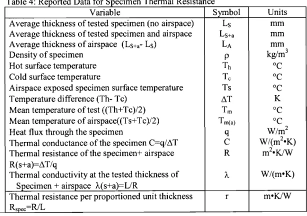
3.5.2 Thermal Resistance of Low Emissivity Sheet Material and Airspace(s) The following collected and calculated data should be provided in the test

report. For the test with the respective (3,6,9 mm) airspaces in place where the

thermal resistance of the material and the airspace(s) are measured, the data

provided should be as outlined in Table 4.

Table 4: Reported Data for Specimen Thermal Resista

Variable

Average thickness of tested specimen (no airspace) Average thickness of tested specimen and airspace Average thickness of airspace (Ls+,- Ls)

Density of specimen Hot surface temperature Cold surface temperature

Airspace exposed specimen surface temperature Temperature difference (Th- Tc)

Mean temperature of test ((Th+Tc)/2) Mean temperature of airspace((Ts+Tc)/2) Heat flux through the specimen

Thermal conductance of the specimen C=q/AT Thermal resistance of the specimen+ airspace R(s+a)=AT/q

Thermal conductivity at the tested thickness of

Ice Symbol Ls Ls+a LA P Th Tc

Specimen + airspace h(s+a)=L/R

Thermal resistance per proportioned unit thickness r

3.6 Calculation of Emissivity

Units

I

Consider two plane surfaces in space, set at an infinite distance of "La" apart. A plane surface, Plate 2 (typical of the hot plate in the Heat Flow

Apparatus) emitting radiant heat "q" would have a known emittance of E, = 0.9

and a known steady state temperature of T2. The plane surface (Plate 1) in parallel with the radiant heat emitting surface (Plate 2), would have an unknown

emissivity of E , and a known steady state surface temperature of T I . If the two

plane objects of equal size were facing each other and if the plane surfaces were large in relation to to the distance between them, then the net heat exchange between the two surfaces would be by radiation only. Given that the heat transfer would be occurring in a vacuum and that the distance between the plates was infinity, it could be concluded that all heat transfer would occur as a result of radiation. There could be no conductive or convective component to the heat transfer.

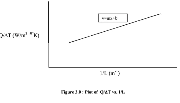
By plotting the results of section 3.5.2 in graphical form for data points of 3,6,9 mm airspaces (inverse) as shown in Figure 2.0, a linear equation could be derived.

Figure 3.0 : Plot of QIAT vs. I&

The x-axis of Figure 3.0 represents the inverse of the distance between the plane surfaces whereas the y-axis represents the heat transfer rate over the

temperature difference between both plates. The y intercept "b" represents the total (i.e. radiant) heat transfer between both plates over the temperature difference between both plates.

Heat transfer across air is by three modes namely conduction, convection and radiation. By combining conduction and convection it can be expressed as:

Qrorol = Qcond-con" + Q ~ a d (eqn. 1.0)

(eqn. 2.0)

Where Q t o t a / = total heat flow, W

Q ~ o n d - C O ~ F conductive-convective heat, W

q=total heat flow per unit area, w/m2

A= area of plates, m2

k= conductivity of air at mean temperature, W/ (m OK)

a= _{Stefan-Boltzman constant, 5.6697 x W/(m2 K4)}

TI= surface temperature of Plate 1 (K)

T2= surface temperature of Plate 2 (K)

E/ = emissivity of Plate 1 surface facing Plate 2

EJ = emissivity of Plate 2 surface facing Plate 1

In the case of the Heat Flow Meter used as per section 3.5.2, although not in a vacuum, the plates are quite close together and are oriented horizontally. This would make the conductive-convective element of heat transfer negligible. Therefore the conductive-convective component of equation 2.0 could be dropped. The simplified equation could be expressed as:

(eqn. 3.0)

The equation could be further simplified and expressed as:

(eqn 4.0)

Where Qr = total heat flow(radiant), W

o= Stefan-Boltzman constant, 5.6697 x 1

o - ~

A T / = surface temperature difference between Plate 1 & 2

(K)

EI = emissivity of Plate 1 surface facing Plate 2

Given that the emissivity of the heating plate in the Heat Flow Apparatus is of

known value, namely ~ 2 = 0.9, equation 4.0 could be further simplified and

expressed in terms of EI by:

The results collected from the Heat Flow Meter as outlined in section 3.5.2 should be plotted as in the configuration of Figure 2.0. The Y intercept Qr/AT would represent the total heat flow over the mean temperature of the two planar surfaces set at an infinite distance apart. There would be three data points, one for each airspace. TM is the mean air temperature is is of the 3,6 and 9 mm airspaces. From equation 5.0, EI, the emissivity of the low emissivity sheet material could be determined.

4.0

Full Scale Modeled Thermal Evaluation

4.1 Field Applications

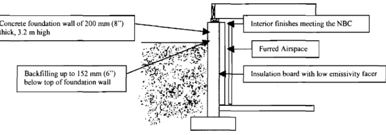
CCMC requested that the three possible field applications shown in Figures

4.0, 5.0 & 6.0, be examined for wall system thermal performance. If the systems

were to be evaluated in a Guarded Box, what test set-ups would be required? Would all three field applications require experimental evaluation? Could the testing be simplified and narrowed to one or two set-ups?

I

Interior finishes meeting the NBC

Backfilling up to 152 nun (6") Insulation board with low emissivity facer

below top of foundation wall

-

Concrete foundation wall of 200 mm (8")

t h c k , 3 2 m high

b I n

Backfill~ng up to 152 m m (6") below top of foundat~on wall

lnsulat~on board w ~ t h low e m i s s ~ v ~ t y facer

Fumcd Alrspace

Intenor fin~shes meetlng the NBC

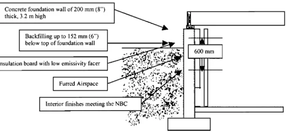
Figure 5.0: Partial Basement Wall System

Insulation board with low emissivity facer

Furred Airspace

Interior finishes meeting the NBC

I

Concrete foundation wall of 200 mrn (8") _{No backlilling higher than the slab} thick, 3.2 m high

Given that the principle objective of a full scale evaluation would be to determine the thermal resistance of a low emissivity faced insulated board-furred airspace assembly basement wall system under different boundary conditions, the differing boundary conditions would have to established and considered. Would the

varying weatherside conditions shown in Figures 4.0,5.0 & 6.0 have any great effect

on thermal performance of the wall system when evaluated in a Guarded Box ?

BE&S first decided to undertake one-dimensional thermal modeling for the three field applications. The basic premise of this exercise was to determine the thermal resistance of the low emissivity sheet insulation and furred airspace assembly within the wall system under the three field applications.

A parallel-path isothermal-plane model developed by BE&S and

experimentally validated was used to carry out the analysis. This model provided the various thermal resistance components throughout the wall system as well as the total thermal resistance. Also provided were the various interstitial temperatures.

4.2 Model Theory

The one-dimensional thermal model developed by BE&S combines both the isothermal plane and the parallel path approach. The average of the two approaches is the modeled thermal resistance of the wall system.

4.1.1 Isothermal Plane Methodology

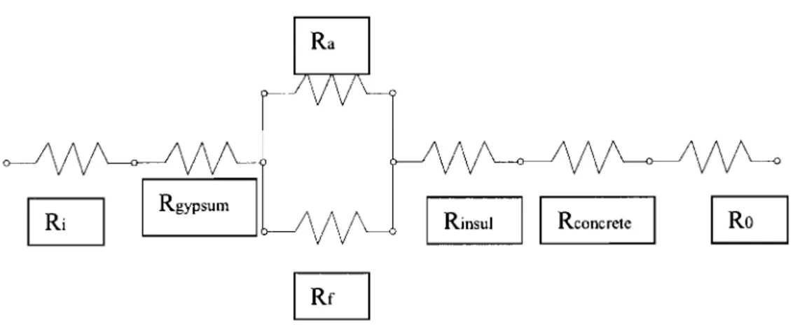
The isothermal plane approach to thermal modeling assumes that each interstitial layer of a wall system has a resultant thermal resistance and uniform interstitial plane temperatures. Using an electrical analogy (Fig 7.0) the various wall element thermal resultant resistances are added in series. The basic thermal

resistances of the wall materials are found in IRC publications and the ASHREA Handbook. Figure7.0 below shows the thermal circuit of the isothermal-plane applied methodology.

Figure 7.0: Isothermal plane thermal circuit of Basement Wall System with Low Emissivity Sheet Insulation and Furred-Airspace.

Where Ri = Thermal resistance of inside film coefficient, 0.12 m2 O W

Rgypsurn = Thermal resistance of 12 mm gypsum, 0.079 m2 O W

Rhmng = Thermal resistance of 19 mm furring, 0.179 m2 O W

Rainpaces = Thermal resistance of 19 mm airspace, 0.597 m2 O W

Rinsu~ = Thermal resistance of 50 mm low E sheet insulation, 1.799 m2 OWW

Rconcrete Thermal resistance of 200 mm concrete, 1.799 m2 OWW

R,,= Thermal resistance of weatherside film coefficient, 0.03 m2 O W

4.1.2 Parallel Path Methodology

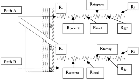
The parallel plane approach to thermal modeling outlines that each thermal path within a wall system has a total thermal resistance. Each path also has a surface area that is a portion of the total wall specimen area. In the most basic terms, the various path thermal resistances are multiplied by their respective percentile areas in relation to total specimen wall area. The portional values are then summed. Using an electrical analogy as shown in Figure 8.0, the various wall element thermal resultant resistances are added in series. The basic thermal

resistances of the wall materials are found in IRC publications and the ASHREA Handbook. Figure 6.0 below shows the thermal circuit of the Isoplanar applied methodology.

Figure 8.0: Parallel-Path thermal circuit of Basement Wall System with Low Emissivity Sheet Insulation and Furred Airspace.

4.2 Model Boundary and Construction Conditions.

4.2.1 Full Basement Wall System

The weatherside boundary conditions of the full basement wall system (Figure 4.0) would first have to be established in view of testing such an assembly in a Guarded Box Facility with a 2438mm X 2438 mm specimen area. Given the geometry of the test area as well as the consideration for area weighed surface instrumentation (i.e. surface thermocouple locations) BE&S concluded that the test wall would be divided into five horizontal sections of 488 mm high (19" each). The top section would be above grade and would be exposed to the cold air climate. The four descending below grade sections would be at temperatures based on real data collected at CCHT.

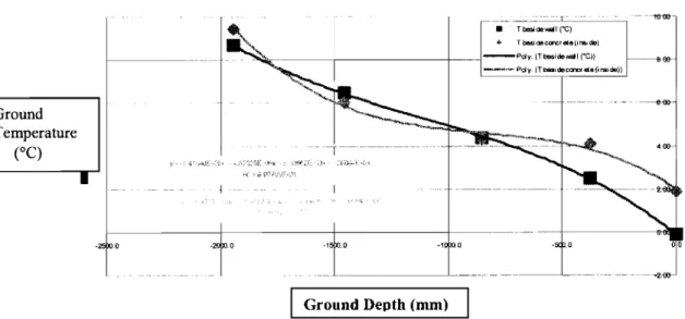
Figure 9.0 below,the plot of CCHT Ground Temperature vs. Depth, provides an actual ground temperature readings at and near a basement wall located under the test house. From this graph, BE&S established the soil and weather side temperature profile for a 2438mm X 2438mm Guarded Box test wall.

Figure 10.0 shows the area weighed level zones with their respective average zone temperatures. The mean area weighed weather-soil side temperature was -2.16 "C. The roomside temperature was 20 "C.

CCHT Ground T e m p e r a t u r e V S D e p t h

I

I

Ground Depth (mm)

Level 1

m-

-

Figure 10.0: Profile of 2438mm X 2438 mm test wall with horizontal area weighed level zones and respective average zone temperatures.

For modeling purposes:

The airspace surface emissivity of the low emissivity surface board insulation was set at 0.05, which is based on the ASHREA handbook standard for bright aluminium (Table 2B pg 23.5, 1985).

Horizontally oriented 1" X 3" furring set on 24" centers was the

strapping set-up.

4.2.2 Partial Basement Wall System

As per Section 4.2.1

4.2.3 Full Basement Wall System With no Backfill

The weather and room side boundary conditions of the full basement wall system with no backfill (Figure 6.0) would follow the ASTM 1363 Standard for Wall Testing in Guarded Hot Boxes, namely a roomside temperature of 20 "C and a

For modeling purposes:

The airspace surface emissivity of the low emissivity surface board insulation was set at 0.05, which is based on the ASHREA handbook standard for bright aluminium (Table 2B pg 23.5, 1985).

Horizontally oriented 1" X 3" furring set on 24" centers was the strapping set-up.

4.3 Modeling Results

4.3.1 Full Basement Wall System

Rwa11= 2.55 RSI

m

m

I

Figure 11: Interstitial temperature profile (airspace path) and thermal resistance for Full Basement Wall System

The Full Basement Wall system was modeled (Figure 4.0). The wall thermal

resistance was 2.55 m2 Om.The thermal resistance of the airspace was

0.599 m2 OK/W. The resultant thermal resistance of the furred-airspace was

0.423 m2 O m , which accounts for 16.5 % of the total thermal resistance.

4.3.2 Partial Basement Wall System

Based partially on the results of section 4.3.1, the Partial Basement Wall system had a calculated thermal resistance of 1.33 m2 O W . This is due to the fact that only the top 1083 mm of the concrete wall is insulated as per Figure 10 and the bottom 1355 mm of the wall is insulated with a 70 mm airspace and 12 thick gypsum board.

When the low emissivity surface of the airspace is removed, the thermal resistance

Of the wall system drops to 1.26 m2 O W .

4.3.3 Full Basement Wall System With No Backfill

Gypsum 12 mm

m

I

m

Figure 12: Interstitial temperature profile (airspace path) and thermal resistance for Full Basement Wall System with no backfill.

The Full Basement Wall System without backfill was modeled (Figure 6.0). The wall thermal resistance was 2.63 m2 O W . The thermal resistance of the airspace

was 0.609 m2 O W . The resultant thermal resistance of the furred-airspace was

4.3.4 Full Basement Wall System With High Emissivity Sheet Insulation

In order to estimate the contribution of the low emissivity surface towards the thermal resistance of the wall system, BE&S modeled the Full Basement Wall System fitted with the same sheet insulation without it's low emissivity surface. The substituted emissivity was 0.9.

Rwal~ = 2.25 RSI

m

Gypsum 12 mm

m

Furred Airspace 19 mm

Figure 13: Interstitial temperature profile (airspace path) and thermal resistance for Full Basement Wall System with no backfill and a high emissivity surfaced sheet insulation.

The Full Basement Wall System without the low emissivity surface in the

airspace was modeled (Figure 6.0). The wall thermal resistance was 2.25 m2 OW.

The thermal resistance of the airspace was 0.1633 m2 OWW. The resultant thermal

resistance of the hrred-airspace was 0.166 m2 OKIW, which accounted for 7.4 % of

4.3.5 Full Basement Wall System With No Backfill & High Emissivity Sheet Insulation

In order to estimate the contribution of the low emissivity surface towards the thermal resistance of the wall system, BE&S modeled the Full Basement Wall System with no backfill fitted with the same sheet insulation without it's low emissivity surface. The substituted emissivity was 0.9.

Rwa11= 2.29 RSI

m

Concrete 403 mm

E I I

Furred Airspace 19 mm _{Tconc= -29.0 OC}

Figure 14: Interstitial temperature profile (airspace path) and thermal resistance for Full Basement Wall System with no backfill and a high emissivity surfaced sheet insulation.

The Full Basement Wall System without backfill and without low emissivity surface in the airspace was modeled (Figure 6.0). The wall thermal resistance was

2.29 m2 O W . The thermal resistance of the airspace was 0.1751 m2 O W . The

resultant thermal resistance of the furred-airspace was 0.176 m2 O W , which

4.3.6 Contribution of Low Emissvity Surface Towards Thermal Resistance of the Full Basement Wall System

Comparing the results of Sections 4.3 1 and 4.3.4, the low emissivity surface

in the furred airspace raised the thermal resistance of the wall assembly from

2.25 m2 O Wto 2.55 m2 O W . Therefore it's contribution to total thermal

resistance was 0.30 m2 O W(1 1.8 % of total).

4.3.7 Contribution of Low Emissvity Surface Towards Thermal Resistance of the Full Basement Wall System

Comparing the results of Sections 4.3 1 and 4.3.4, the low emissivity surface in the furred airspace raised the thermal resistance of the wall assembly from

1.26 m2 O Wto 1.33 m2 O W . Therefore it's contribution to total thermal

resistance was 0.07 m2 O W(5.3 % of total).

4.3.8 Contribution of Low Emissvity Surface Towards Thermal Resistance of the Full Basement Wall System With no Backfill.

Comparing the results of Sections 4.32 and 4.33, the low emissivity surface in the furred airspace raised the thermal resistance of the wall assembly from

2.29 m2 OWW to 2.63 m2 O W . Therefore it's contribution to total thermal

4.3.9 Summary of Modeled Results

Table 5.0 Summar of Thermal Modelin Results

Wall System T~oornside Tweatherside Thermal (m2 O w

Full Basement Wall

System with (Fig 4.0) with no foil surface on sheet insulation.

1

I

1

1

1

System with (Fig 5.0) and with no foil surface System (Fig 5.0)

Partial Basement Wall

System with no backfill (Fig 6.0)

20.0

4.3.10 Discusion of Modeled Results

Full Basement Wall System with no backfill (Fig 6.0) and with no foil surface on sheet insulation.

The weatherside temperature differences barely affected the thermal

resistances of the fully insulated test wall. The variance was only 0.08 m2 O W , or

about 3 % of the total thermal resistance of the wall system. Given that the error of

a typical Guarded Box is in the order of 6 %, these differences would not likely be

detected.

In the case of the Partial Basement System where only the top half of the wall is insulated, the experimenter would likely confuse results by introducing two different walls into one specimen.

-2.1

4.3.1 1 Conclusions of Modeled Results

1.27

20.0

Based on modeled results of little variance, BE&S concludes that only one of the three field applications needs to be evaluated. The simplest wall to evaluate would be the Full Basement Wall System with no backfill (Fig 6.0).

5.0

Full Scale Experimental Thermal Evaluation

5.1.1 Specimen Construction

A 2438 mm X 2438 mm test specimen that includes a 200 mm thick concrete slab would be both difficult to build and to mount in a Guarded Box. If a lighter material of similar thermal resistance to that of concrete could be substituted, it would simplify the experiment. A concern however was that two-dimensional heat transfer might occur in the concrete slab during testing thereby nullifying the validity of the one-dimensional thermal model used for analytical purposes.

BE&S has determined that two dimensional heat transfer would not be a concern if the weatherside temperature was constant over the weatherside surface of the specimen. This was verified by concrete wall tests carried out by IRC for ASHREA a number of years ago. Given that BE&S concludes that only one wall system needs to be evaluated, namely the Full Basement Wall System with no backfill (Fig 6.0), then the weatherside temperature would be uniform and thus two dimensional heat transfer through the concrete slab would not occur in any measurable quantity. For this reason, 30 mm thick plywood could be used in place of the concrete slab. Figure 15.0 below shows the typical test wall profile. The orientation of the strapping could be vertical or horizontal.

Airsnace 1 9 mm

The Full Basement Furred-Airspace Test Wall would be a layered 2.44 m X 2.44 m assembly consisting of 200 mm low emissivity board insulation affixed to a 30 mm thick layer of plywood. 19.1 mm furred airspace would be created by affixing nominal 1" X 3" pine strapping (either vertically or horizontally) spaced at either 406 or 61 0 mm over the board insulation. A 12 mm layer of gypsum would then be affixed over the strapping.

5.1.2 Base Case Wall

An objective of the experiment is to experimentally determine the specific thermal resistance of the furred airspaces with one low emissivity surface. In order to carry this out, a wall similar to that profiled in Figure 15.0,except that the low emissivity surface of the sheet insulation would not be in place. This could be called the Base Wall System.

By subtracting the thermal resistance of BaseWall System from that of the Full Basement Wall System, the thermal resistance contribution of the low emissivity surface (in a furred airspace) would be determined.

5.1.3 Furring Details

There are two variants in the fumng details of the test walls

Fumng Spacing: The fumng strips could be spaced typically 406 mm (16") or 61 0 mm (24") apart.

Fumng Orientation: The fumng strips could be oriented either vertically or horizontally.

Vertical Orientation: Convective heat transfer within the airspace would be more likely if the furring were mounted vertically. Considering the field applications (see figures 4.0 to 6.0) where the floor (typical 112" space at bottom of gypsum) and ceiling (112"X 16" or 24" openings between strapping) details are open, a vertical heat path would be created up through the furred airspace(s). In this case, two-dimensional heat flow might occur and a one-dimensional thermal might not be valid for analysis. Two dimensional heat flow could be experimentally determined by instrumenting the center airspace with thermocouples from top to bottom and observing if any significant thermal gradient exists. Given that edges are sealed for Guarded Box specimen, these top and bottom opening details would have to be included in the test

specimen. Vertical orientation of strapping would require that slots of 19 mm X 2438 mrn at the top, and 25 mm X 2438 mm at the bottom be cut on the roomside of the specimen in order to allow for any vertical thermal gradient that might occur.

Horizontal Orientation: Convective heat transfer within the airspace would not be likely if the fumng were mounted horizontally. In this case two dimensional heat flow would not be likely and the one-dimensional thermal model could be used for analysis.

5.1.4 Test Method

The standard test method for determining the thermal performance of walls is ASTM C-1363. For the purposes of this test, this method should be followed. The weatherside temperature would be maintained at -35 "C. The roomside temperature would be maintained at 20 OC. The heat resistance value would be measured and calculated from roomside wall surface to soil-weatherside wall surface.

5.15 Instrumentation

Twenty temperature measuring thermocouples would be affixed to the respective outer wall surfaces in an area weighed layout in order to determine the thermal resistance of the basement wall assembly (Fig 16.0). Additional

thermocouples would also be mounted in the interstitial layers of the wall assembly (Figs 1 1.0 to 14.0). In order to provide temperature profiles across the wall at five different vertical levels, the wall would be divided into five horizontal level zones of 484 mm deep. The interstitial thermocouples would be mounted in the middle of each level. Strapping orientation would not alter thermocouple locations.

Fig 16.0: Instrumented Full Basement Wall System

L e v e l I (obove g r o d e ) L e v e l 2 . -. L e v e l 3 - . .- -. L e v e l 4 L e v e l 5 T C - 0 1 T C - 0 2 T C - 0 3 T C - 0 4

+

+

+

+

+

+

+

+

+

+

+

+

+

+

+

+

+

+

+

+

6.0 Conclusions

Two full scale walls should be evaluated in a Guarded Hot Box under the following conditions: The weatherside temperature should be set at -35 OC and the roomside temperature should be set at 20 OC (ASTM C-1363). The concrete slab should be replaced with 30 mm plywood sheathing One wall (Full Basementwall System) should be fitted with the low emissivity sheet insulation.

The other wall (Base Wall System) should be fitted with the same sheet insulation without it's low emissivity surface.

The thermal resistance created by the low emissivity surface within the furred airspace can be determined by subtracting the thermal resistance of the Base Wall from the thermal resistance of the Full Basement Wall System.

Airspace strapping could be oriented vertically or horizontally but

instrumentation should be set up in order to detect two-dimensional heat flow. Vertical orientation of strapping will require that slots of 19 mm X 2438 mm at the top, and 25 mm X 2438 mm at the bottom be cut on the roomside of the specimen.