Publisher’s version / Version de l'éditeur:
Technical Report, 2008-01-01
READ THESE TERMS AND CONDITIONS CAREFULLY BEFORE USING THIS WEBSITE. https://nrc-publications.canada.ca/eng/copyright
Vous avez des questions? Nous pouvons vous aider. Pour communiquer directement avec un auteur, consultez la première page de la revue dans laquelle son article a été publié afin de trouver ses coordonnées. Si vous n’arrivez pas à les repérer, communiquez avec nous à [email protected].
Questions? Contact the NRC Publications Archive team at
[email protected]. If you wish to email the authors directly, please see the first page of the publication for their contact information.
Archives des publications du CNRC
For the publisher’s version, please access the DOI link below./ Pour consulter la version de l’éditeur, utilisez le lien DOI ci-dessous.
https://doi.org/10.4224/20178996
Access and use of this website and the material on it are subject to the Terms and Conditions set forth at
Thickness and material properties of multi-year ice sampled during the CAT study, August 2007
Johnston, M.
https://publications-cnrc.canada.ca/fra/droits
L’accès à ce site Web et l’utilisation de son contenu sont assujettis aux conditions présentées dans le site
LISEZ CES CONDITIONS ATTENTIVEMENT AVANT D’UTILISER CE SITE WEB.
NRC Publications Record / Notice d'Archives des publications de CNRC: https://nrc-publications.canada.ca/eng/view/object/?id=8d889fc2-f524-448b-9f2d-e0ef9bde85e6 https://publications-cnrc.canada.ca/fra/voir/objet/?id=8d889fc2-f524-448b-9f2d-e0ef9bde85e6
Thickness and Material Properties of Multi-Year Ice
Sampled during the CAT Study, August 2007
M. Johnston
Technical Report, CHC-TR-067
January 2008
Thickness and Material Properties of Multi-Year Ice Sampled
during the CAT Study, August 2007
M. Johnston
Canadian Hydraulics Centre National Research Council of Canada
Montreal Road Ottawa, Ontario K1A 0R6
prepared for:
Transport Canada
Transport Canada, Marine Safety 330 Sparks St., 10th floor (AMSRP), Tower C, Place de Ville
Ottawa, ON
Program of Energy Research and Development (PERD) Natural Resources Canada
580 Booth St. Ottawa, ON
Canadian Ice Service Environment Canada Marine and Ice Services
373 Sussex Drive Ottawa ON
Technical Report, CHC-TR-067
Abstract
A field program was carried out to measure the properties of multi-year ice in the high Arctic. Thicknesses are reported for multi-year ice floes in Nares Strait (9 floes), Norwegian Bay (1 floe) and Lady Anne Strait (1 floe). The diameter of the 11 floes ranged from 175 m to 7.5 km. Multi-year ice in mainstream Nares Strait drifted south at 1.38 to 2.04 km/hr in a near-straight trajectory. The trajectories of two floes were mapped using satellite tracking beacons. Floe N06, which had an average thickness of more than 9.5 m but was only about 500 m in diameter, drifted south from Nares Strait until it disintegrated along the eastern coast of Baffin Island almost two months later. Floe N08 was a 2.8 km diameter floe that had an average thickness of more than 8.7 m. The beacon on Floe N08 continues to transmit at the time of writing this report, six months later, off the eastern coast of Baffin Island.
More than 1500 m of ice was drilled during the program. Five of the floes had an average thickness of more than 7.7 m, whereas the average thickness of the other six floes ranged from 3.6 to 5.9 m. Standard deviations in thickness on the 11 floes ranged from 0.7 to 3.7 m. The temperature and salinity of the multi-year ice was measured on 4.80 to 5.50 m long cores. The top ice surface was the warmest (-0.9°C) and the interior of the ice was the coldest (-6.9°C). The average temperature of the ice cores ranged from -2.6°C to -4.7°C. Salinities in the uppermost 60 to 100 cm of ice were negligible (0 to 0.2 ‰) and increased to a maximum of 3.6 ‰ towards the interior of the ice. Most of the floes had an average salinity that was quite uniform (1.0 to 1.7 ‰). Borehole strengths were conducted on five floes. The strength was lowest in the uppermost 60 cm of ice (4.0 to 11.5 MPa) and generally increased with increasing depth to 21.5 to 30.6 MPa. The average borehole strength was remarkably consistent on four of the floes (15.9 to 17.5 MP). One floe had an average borehole strength of 23.1 MPa. Comparison of the strength and temperature profiles for the different floes illustrate the inverse relation between temperature and strength.
ScanSAR and Standard imagery from RADARSAT-1 were examined to determine whether individual floes were recognizable. Standard imagery was preferred over ScanSAR imagery because of its higher resolution (25 m vs. 150 m). ScanSAR images adequately captured multi-year ice floes upwards of 4.0 km in diameter, but they were not useful for identifying floes less than several kilometers across. In comparison, floes from 400 to 500 m across were detectable in the Standard images, except for when they were masked by the high concentrations of pack ice.
Résumé
Une étude de terrain a été effectuée dans le but de mesurer les propriétés de la glace pluri-annuelle dans le Haut-Arctique. Dans ce rapport, on présente des données sur l’épaisseur de neuf (9) floes dans le détroit de Nares, de un (1) floe dans la baie Norwegian et de un (1) floe dans le détroit de Lady Anne. Le diamètre de ces 11 floes se situait entre 175 m et 7,5 km. La glace pluri-annuelle dans l’axe du détroit de Nares a dérivé vers le sud suivant un tracé à peu près rectilinéaire, à une vitesse de 1,38 à 2,04 km/h. La trajectoire de deux floes a été suivie par satellite, par l’intermédiaire de radio-balises. Le floe N06, d’épaisseur moyenne de plus de 9,5 m mais dont le diamètre n’était que d’environ 500 m, a dérivé vers le sud depuis le détroit de Nares, jusqu’à son démantèlement presque deux mois plus tard le long de la côte est de l’île de Baffin. Le floe N08 avait un diamètre de 2,8 km et une épaisseur moyenne de plus de 8,7 m. La transmission de données de la radio-balise sur ce floe était encore en cours durant la rédaction de ce rapport, six mois plus tard, depuis la côte est de l’île de Baffin.
Durant cette étude, on a foré sur une longueur cumulative totale de plus de 1500 m. Cinq des 11 floes avaient une épaisseur de plus de 7,7 m; l’épaisseur moyenne des autres allait de 3,6 à 5,9 m. L’écart-type pour l’ensemble des floes variait de 0,7 à 3,7 m. On a également mesuré la température et la salinité de la glace multi-annuelle sur des carottes de 4,80 à 5,50 m de longueur. La température à la surface du floe était la plus élevée (-0,9oC) et diminuait par la suite (jusqu’à un minimum de -6,9oC). La température moyenne des carottes variait de -2,6oC à -4,7oC. La salinité de la glace, négligeable à 60-100 cm de la surface (0 à 0,2 ‰), atteignait 3,6 ‰ par la suite. On a constaté que la salinité moyenne de la plupart des floes était relativement uniforme (1,0 à 1,7 ‰). La résistance de la glace dans les trous de forage a été mesurée sur cinq floes. Elle était la moins élevée (4,0 à 11,5 MPa) à 60 cm de la surface, et augmentait avec la profondeur jusqu’à des valeurs de 21,5 à 30,6 MPa. La résistance moyenne de la glace sur quatre floes était étonnamment uniforme (15,9 à 17,5 MPa). Sur un des floes, elle atteignait 23,1 MPa. On observe une relation inverse entre la résistance et les profils thermiques sur chacun des floes. On a procédé à l’examen d’images radar ScanSAR et Standard de RADARSAT-1 pour savoir si on pouvait y distinguer ces floes. L’imagerie Standard était préférable à ScanSAR, en vertu d’une meilleure résolution (25 m plutôt que 150 m pour ScanSAR). Pour retracer les floes dont le diamètre dépassait 4,0 km, les images ScanSAR étaient adéquates. Mais elles ne se sont pas avérées utiles pour les floes dont la dimension était inférieure à quelques kilomètres. Par contre, sur les images Standard, on arrivait à identifier des floes dont la dimension se situait entre 400 à 500 m, sauf dans les cas où ces floes ne se démarquaient pas suffisamment de la banquise environnante (lorsqu’elle était particulièrement dense).
Table of Contents
Abstract ... i
Résumé...iii
Table of Contents... v
List of Figures ...vii
List of Tables ... ix
1.0 Introduction... 1
1.1 Reports Issued for this Project ... 2
2.0 Voyage Information and Study Area ... 2
3.0 Floe Selection Process ... 5
3.1 RADARSAT Imagery... 5
4.0 Location of Sampling Sites... 6
5.0 Results from Field Study ... 8
5.1 Floe N01... 9 5.1.1 Satellite View... 12 5.2 Floe N02... 13 5.2.1 Satellite View... 15 5.3 Floe N03... 16 5.3.1 Satellite View... 18 5.4 Floe N04... 19 5.4.1 Satellite View... 22 5.5 Floe N05... 23 5.6 Floe N06... 26
5.6.1 Temperature and Salinity Profiles ... 26
5.6.2 Satellite View... 29
5.6.3 Beacon Installation on Floe N06 ... 29
5.7 Floe N07... 31
5.7.1 Temperature, Salinity and Strength Profiles... 31
5.7.2 Satellite View... 34
5.8 Floe N08... 35
5.8.1 Temperature, Salinity and Strength Profiles... 35
5.8.2 Satellite View... 36
5.8.3 Beacon Installation on Floe N08 ... 36
5.9 Floe N09... 40
5.9.1 Temperature, Salinity and Strength Profiles... 40
5.10 Floe N10... 43
5.10.1 Temperature, Salinity and Strength Profiles... 43
5.10.2 Satellite View... 46
5.11 Floe N11... 47
5.11.1 Temperature, Salinity and Strength Profiles... 47
5.11.2 Satellite View of Floe N11 ... 50
6.0 Summary ... 51
6.1 Temperature, Salinity and Strength ... 51
6.1.1 Temperature ... 51
6.1.3 Strength ... 52 6.2 Ice Thickness ... 53 6.3 Satellite Imagery ... 54 7.0 Conclusions... 55 8.0 Acknowledgments... 56 9.0 References... 57 Appendix A: Equipment and Methodology... A-1
Ice thickness measurements using the drill hole technique ... A-3 Ice Property Measurements ... A-3 Appendix B: Particulars of Satellite Imagery used in Report... B-1
List of Figures
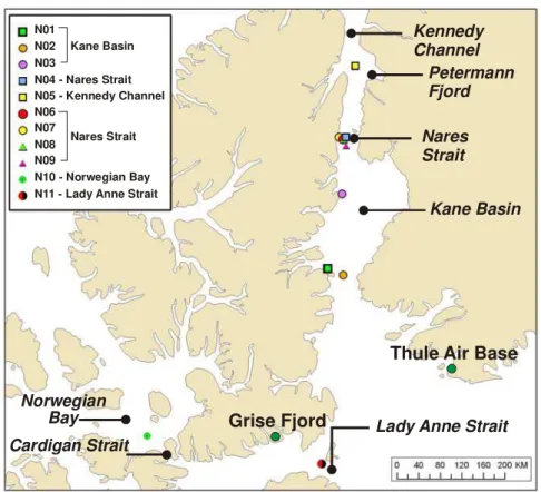
Figure 1 Points of interest during CAT Study, 2007. ... 3
Figure 2 Locations of multi-year ice floes sampled in August 2007... 7
Figure 3 Three of the boxes of equipment that were retrieved from Alexandra Fjord... 9
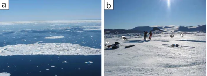
Figure 4 Floe N01 from the (a) air and (b) ice... 11
Figure 5 Floe N01 (a) plan view of thickness transects and (b) sail and keel profiles. ... 11
Figure 6 ScanSAR image showing initial and final position of Floe N01, Alexandra Fjord. ... 12
Figure 7 Floe N02 from the (a) air and (b) ice... 14
Figure 8 Floe N02 (a) plan view of transects and (b) corresponding sail and keel profiles. ... 14
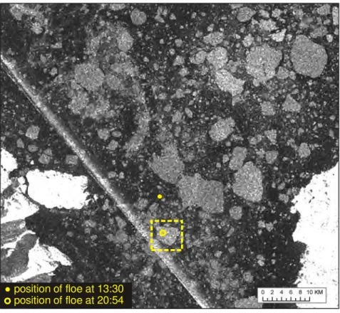
Figure 9 ScanSAR image showing initial and final position of Floe N02, Smith Sound... 15
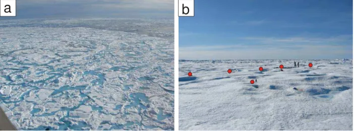
Figure 10 Floe N03 from the (a) air and (b) ice... 17
Figure 11 Floe N03 (a) plan view of transects and (b) corresponding sail and keel profiles. ... 17
Figure 12 Standard image showing initial position of Floe N03 outside Scoresby Bay. ... 18
Figure 13 Floe N04 (a) ice surface along Transect 1 and (b) retrieving a core. ... 20
Figure 14 Floe N04 (a) plan view of transects and (b) corresponding sail and keel profiles. ... 20
Figure 15 Temperature and salinity profiles of Floe N04. ... 21
Figure 16 ScanSAR image showing initial and final position of Floe N04, Nares Strait ... 22
Figure 17 Floe N05 (a) from the air and (b) level surface along the main transect... 24
Figure 18 Floe N05 (a) plan view of transects and (b) corresponding sail and keel profiles. ... 24
Figure 19 Temperature and salinity profiles of Floe N05. ... 25
Figure 20 Floe N06 from the (a) air and (b) ice... 27
Figure 21 Floe N06 (a) plan view of transects and (b) corresponding sail and keel profiles. ... 27
Figure 22 One happy man, after having labored to retrieve the corer for two hours! ... 28
Figure 23 Temperature and salinity profiles in the uppermost metre of ice at Floe N06... 28
Figure 24 Standard image containing Floe N06, Nares Strait. ... 29
Figure 25 Trajectory of Floe N06 from 20 August 2007 to 3 October 2007... 30
Figure 26 Floe N07 from the (a) air and (b) ice... 32
Figure 27 Floe N07 (a) plan view of transects and (b) sail and keel profiles... 32
Figure 28 Temperature, salinity and strength of Floe N07... 33
Figure 29 Standard image showing initial and final position of Floe N07... 34
Figure 30 Floe N08 from the (a) air and (b) ice... 37
Figure 31 Floe N08 (a) plan view of transects and (b) sail and keel profiles... 37
Figure 32 Ice temperature, salinity and strength of Floe N08. ... 38
Figure 33 Standard image showing initial and final position of Floe N08... 38
Figure 34 Trajectory of Floe N08 from 24 August 2007 to 30 January 2008. ... 39
Figure 35 Floe N09 from the (a) air and (b) ice... 41
Figure 36 Floe N09 (a) plan view of drilled holes and (b) corresponding sail and keel profiles.41 Figure 37 Temperature, salinity and strength of Floe N09... 42
Figure 38 Floe N10 from the (a) air and (b) ice... 44
Figure 39 Floe N10 (a) plan view of transects and (b) corresponding sail and keel profiles. ... 44
Figure 40 Temperature, salinity and strength of Floe N10... 45
Figure 41 Images containing Floe N10, sampled on 29 Aug 2007, 12:51 to 21:29UTC. ... 46
Figure 42 Floe N11 from the (a) air and (b) ice... 48
Figure 43 Floe N11 (a) plan view of transects and (b) corresponding sail and keel profiles. ... 48
Figure 45 ScanSAR image showing initial and final position of Floe N11. ... 50 Figure 46 Average thickness and diameter of 11 multi-year ice floes ... 53
List of Tables
Table 1 Floes sampled during 2007 Field Study ... 8 Table 2 Summary of Property Measurements1... 52
Thickness and Material Properties of Multi-Year Ice Sampled
during the CAT Study, August 2007
1.0 Introduction
Multi-year ice was the focus of this work. Multi-year ice results in the greatest number of damage events on ships (Kubat and Timco, 2003) and causes the highest loads on offshore structures (Timco and Johnston, 2004). Relatively little is known about its thickness, strength, failure modes and driving force however. The objective of this field study was to obtain a representative picture of the multi-year ice that originates in the polar pack and exits through Kennedy Channel. Many of those floes eventually move south to become a hazard for ships. In this study, multi-year ice was characterized by the following means:
(1) detailed measurements of multi-year ice thickness using the drill hole technique (2) depth profiles of the strength, temperature and salinity of the ice
(3) asses the feasibility of using ground-based electromagnetic induction sensors for measuring the thickness of multi-year ice
(4) use on-ice measurements to validate the signature of multi-year ice in RADARSAT imagery (5) deploy satellite beacons on two multi-year ice floes to track their migration
This Joint Industry Project (JIP) was made possible through the support of Transport Canada, the Program for Energy Research and Development (PERD), ConcocoPhillips Canada Resources Corp., ExxonMobil Upstream Research Co and Canadian Ice Service. The work follows upon the ice decay-related measurements that the Canadian Hydraulics Centre of the National Research Council Canada (CHC-NRC) has been conducting for Transport Canada for the past several years, in support of the Arctic Ice Regime Shipping System (AIRSS). The results are of interest to the Government of Canada (through the CCTII program and PERD) because recent field measurements on year ice are needed to determine whether the thickness of multi-year ice has been altered by Climate Change. The work is also relevant to ExxonMobil and ConocoPhillips because it seeks to address the question, “Does very thick multi-year ice still exist?”. While each supporting organization may have had slightly different motives in funding this work, all organizations benefit from each others’ objectives.
The multi-year ice study was linked to a larger project entitled the Canadian Arctic Throughflow (CAT) Study, which is championed by Dr. Humfrey Melling at DFO-IOS. The CAT Study was sanctioned by the Canadian Government as part of the International Polar Year (http://www.ipy-api.gc.ca/intl/fs/cat_e.html). Logistical support for the on-ice measurements was made possible by collaborating with the Department of Fisheries and Oceans Institute of Ocean Science (DFO-IOS).
The Canadian Ice Service (CIS) provided a considerable amount of in-kind support for the work. One of their mandates is to support IPY sanctioned projects. CIS has a strong interest in this work because multi-year ice has become one of their key areas of interest (R. DeAbreu, personal communication). The on-ice measurements provided an excellent opportunity for them to have satellite imagery validated, and also for CIS to obtain a better understanding of the properties and migration of multi-year ice.
1.1 Reports Issued for this Project
Two reports were issued for this project: one for the Canadian Government and the another for Private Industry. This publicly available “Thickness and Material Properties of Multi-Year Ice Sampled during the CAT Study, August 2007” focuses on the thickness, temperature, salinity and strength measurements that were made during the CAT Study.
2.0 Voyage Information and Study Area
Research during the Canadian Arctic ThroughFlow (CAT) Study was conducted from the CCGS
Henry Larsen in Nares Strait and Cardigan Strait/Hell Gate (Figure 1). The CAT Study is the culmination of ten years effort within the Canadian and international scientific community to measure flows of seawater and ice through the Canadian Arctic Archipelago (Melling, 2007). Since tracking the thickness and movement of sea ice is an important component of the CAT Study, Dr. Melling welcomed the opportunity to have the National Research Council’s Canadian Hydraulics Centre (NRC-CHC) participate in the program. The on-ice measurements would add a unique perspective to the CAT study: the thicknesses obtained from the on-ice measurements could be compared to the ice thicknesses from the CAT study’s upward looking sonar.
Thule (Air Base) Pond Inlet Nanisivik Grise Fjord Alexandra Fjord GREENLAND Norwegian Bay Hell Gate/ Cardigan Strait Kennedy Channel Lincoln Sea Kane Basin Jones Sound Lady Anne Strait
Nares Strait
ELLESMERE ISLAND
Figure 1 Points of interest during CAT Study, 2007.
On 8 August 2007, the eight members of the IPY CAT study and the two people from NRC-CHC met in St. Johns’s, Newfoundland. The field party flew from St. John’s to Thule Air Base, Greenland on the plane that the Canadian Coast Guard had chartered for crew change operations. The icebreaker was boarded on the afternoon of 8 August, while docked at the Thule Air Base. Since Commanding Officer Vanthiel and the science party were eager to begin the field program, the ship was underway for the main study area soon after crew change operations had been completed. The urgency was due to the fact that ice conditions in that region are extremely dynamic. At best, there are only a few weeks in August when the multi-year ice in Kane Basin and Nares Strait (Figure 1) is loose enough to allow an experienced captain of an icebreaker to operate comfortably.
The oceanographic work of the IPY-CAT study was demanding, and it made full use of the ship’s Officers and Crew. The on-ice work was secondary, but it also made demands on the Officers and Crew, in effect, detracting from the IPY-CAT study. It was a fine balancing act for Captain Vanthiel to determine when (and how) to support the different science programs, but it was an act that he did exceedingly well. The experience that was during the summer of 2006, the first time that DFO and NRC had used the same ship to assist with two very different field programs in Nares Strait, laid the groundwork for a very successful field season in August 2007. The CCGS Henry Larsen had been contracted for the oceanographic measurements of the CAT Study, which meant that the on-ice measurements needed to be conducted on an opportunity basis. Floes were selected about 15 minutes from the ship (flying time) when possible, to maximize the field party’s time on the ice and to maintain radio communication with the ship. Thanks to the cooperation (and generosity) of Captain Vanthiel and Dr. Melling, the NRC-CHC team was able to sample 11 multi-year ice floes during the program. Generosity is a key descriptor here because the ship patiently waited nearby for the on-ice team to complete their measurements, even when the oceanographic team had completed their work in an area and were ready to move on to different area.
Sampling 11 floes during the 11 days that were made available for on-ice measurements is an excellent track record, considering that about 8 days of the voyage were spent transiting to and from Nares Strait, as described in Appendix A. Typically, the ship steamed around the clock, as it transited to the first study area (Nares Strait and Kennedy Channel) and then south to the second study area (Cardigan Strait and Hell Gate). The eight members of the IPY-CAT study disembarked on 2 September, in Pond Inlet and the NRC-CHC group (the author and Richard Lanthier, her field technician) disembarked in Nanisivik on 4 September 2007 (Figure 1).
3.0 Floe Selection Process
Since multi-year ice was plentiful during the CAT study it was relatively easy to select floes of different sizes and thicknesses. The reason for selecting a variety of ice floes was to gain a better understanding of the different types of multi-year ice that move south from the Lincoln Sea (polar pack) into the Eastern Arctic (Figure 1). While there were a large number of floes to chose from, selecting “the floe” was not usually straightforward. Criteria were developed to quickly assess the thickness of the floe from the air, the helicopter being the most feasible means of accessing the ice. It was imperative that floes be selected promptly because that meant more time could be spent sampling the ice – an important component considering the amount of work that needed to be done on each floe (Appendix B). The floe size, surface roughness, extent of decay/ponding, ice freeboard, presence of dirt on the ice and the amount of weathering were all taken into account when selecting a floe.
The planned approach of sampling relatively thin multi-year ice during the early part of the field study, and graduating to thicker ice later in the study was not realized. Beginning with relatively thin multi-year ice would allow the field equipment to be tested under not-too onerous conditions, while providing experience in the ‘art’ of drilling through late summer multi-year ice. Multi-year ice presents many more challenges for drilling and coring in late summer than it does in spring. Experience soon showed that discriminating ‘thin’ multi-year ice from ‘thick’ multi-year ice was extremely challenging, from both the helicopter or the ship’s bridge. The floes were usually much thicker than they appeared. In fact, the very first floe that was sampled was one of the thickest floes of the field program; the ice was more than 10 m thick in 8 of the 10 drill holes. It soon became apparent that graduating systematically from thin to thick multi-year ice would not be possible. The decision was made to randomly sample floes in the vicinity of the ship early on, and then try to ‘fill-in-the-blanks’ more judiciously as the study continued.
3.1 RADARSAT Imagery
Prior to entering the field, the Canadian Ice Service (CIS) was consulted to request RADARSAT imagery in support of the CAT study, which was one of 44 IPY sanctioned projects. CIS, in turn, held discussions with the Canadian Space Agency (CSA), the receiving station in Gatineau, Quebec and the receiving station at the University of Alaska, Fairbanks to see what could be done. A considerable amount of time and effort on the part of DFO-IOS, NRC-CHC and CIS was spent arranging for 16 high resolution RADARSAT Standard images (25 m resolution) to be made available to the ship in near-real-time. Having the images in near-real-time was crucial because a fresh crop of multi-year ice passes through Kennedy Channel and Nares Strait every day, due to the effects of wind, current and tide. It is not unusual for floes in that area to move 60 km south over the course of one day. CIS worked very hard to ensure that the compressed images were ready to be sent to the ship no more than two hours after the satellite overpass. As it turned out, the images could only be successfully downloaded very early in the morning, which was the only time that an uninterrupted communication link could be established long enough to transfer the data.
In addition to the 16 RADARSAT images that had been specially ordered for the IPY-CAT Study, CIS made available the ScanSAR images that were supplied to the ship on a near-daily basis. The ScanSAR images were crucial for ship operations in that area because they provided the only available information about ice conditions in the area, and the types of ice that would move into the area over the next few days.
It was hoped that the Standard and ScanSAR images could be used to identify floes of interest during the trip, so that the on-ice team could be mobilized in time to sample the ice before the floes moved out of the area. The problem with using satellite imagery to identify floes for on-ice measurements stemmed from the rapidly changing ice conditions in the area – images that are several hours, to one day old are of little use when trying to locate a floe from a helicopter. The satellite imagery could not be used to select floes for sampling, however it was useful for identifying the floe after the fact, provided the satellite passed over the floe while the on-ice measurements were being made. The latitude and longitude from a handheld global positioning system (accuracy 15 m) could be used to successfully identify a feature in the geo-referenced image, provided the image resolution was comparable to the floe diameter. The Standard and ScanSAR images that were used in the report are listed in Appendix C.
4.0 Location of Sampling Sites
The 11 multi-year ice floes that were sampled during the field program were distributed over a huge area that extended from Norwegian Bay in the southwest, to the north end of Kennedy Channel (Figure 2). Three of the floes were sampled in Kane Basin (Floe N01 to N03), while the ship transited to Nares Strait, the main study area. By August 14, the ship was at the principal line of moored instruments in Nares Strait, but not for long because the ship received news that a crew member’s wife was seriously ill that afternoon. The ship abruptly departed on the 700 km trip south to Grise Fjord, the nearest community on Ellesmere Island – a journey that consumed the next four days. The ship returned to Nares Strait late on Friday August 17. The following day, the on-ice team sampled their fourth floe, Floe N04, near the main line of the oceanographic moorings. That evening, the ship again departed from Nares Strait, but this time the journey was to Petermann Fjord, 150 km north, to retrieve several years of data from oceanographic instruments. The trip was urgent because ice conditions along the Greenland side had improved enough to permit a relatively unchallenged transit north, however the situation could change at any time. Last year, a trip to Petermann Fjord had not been possible because Kennedy Channel remained sufficiently clogged with multi-year ice throughout the trip.
The ship reached Petermann Fjord on Sunday morning, August 19. Floe N05 was sampled later that day, while the oceanographic team worked in the area (Figure 2). The ship departed Petermann Fjord that evening and was back on site in Nares Strait on Monday morning, August 20, where it worked for the next six days. That week, the on-ice team visited another four floes, Floes N06 to N09. On August 26, the ship departed for Cardigan Strait, in the southwest corner of Ellesmere Island, which was also an area of interest for the CAT study. The side trip to Cardigan Strait provided the opportunity to sample Floe N10 (Norwegian Bay) and Floe N11 (Lady Anne Strait), which concluded the program on August 31.
Grise Fjord
Thule Air Base Norwegian Bay Cardigan Strait Kennedy Channel Petermann Fjord Kane Basin
Lady Anne Strait Nares Strait N01 N02 N03 N04 - Nares Strait N05 - Kennedy Channel N06 N07 N08 N09 N10 - Norwegian Bay N11 - Lady Anne Strait
Kane Basin
Nares Strait
Figure 2 Locations of multi-year ice floes sampled in August 2007
Table 1 lists some of the particulars of the floes sampled during the field study, such as initial and final positions of the floe, and the time that the ice party arrived and departed from the floe. The amount of time that was spent on any given floe depended upon the time allotted from discussions with Commanding Officer Vanthiel and Chief Scientist Humfrey Melling. In general, the helicopter would ferry the field party to the floe in the morning and return to the floe by about 18:00 hrs. Floes N01, N05 and N06 were the exception, because only the afternoon was available for sampling those floes.
When the sampling period was restricted to an afternoon, the full suite of measurements was ‘pared down’ so that the field party could return to the ship in a timely manner. Experience showed however, that at least 5 hours were required to conduct a decent set of measurements on a floe, although a full day was preferred. The total amount of drift noted in Table 1 was obtained using the initial and final positions of the floe. The calculation is appropriate for floes that followed a near-straight trajectory (floes in Nares Strait and Lady Anne Strait). The total drift of Floe N10 (Norwegian Bay), the only floe that had a circular trajectory, was calculated by summing segments along the trajectory recorded by the global positioning system. The calculated drift speed of the floes varied from 0.69 km/hr (Floe N10) to 2.01 km/hr (Floe N11). The fast moving ice explains why the ship encountered a fresh crop of multi-year ice every day. The weather was excellent during the field program. Most days brought clear skies, a wall of sunshine and minimal wind. Air temperatures during the field program varied from 0 to +6°C.
Table 1 Floes sampled during 2007 Field Study Floe ID date sampled initial position (N, W) final position (N, W) arrival - departure time (UTC)* sampling duration (hrs) total drift (km)** average drift speed (km/hr) N01 Kane Basin 10-Aug (p.m.) 78 49.829 74 30.136 78 48.211 74 25.684 17:43 - 21:38 3.92 3.5 0.89 N02 Kane Basin 12-Aug 78 38.077 73 33.234 78 34.095 73 39.985 13:30 - 20:54 7.40 7.9 1.07 N03 Kane Basin 13-Aug 79 50.216 70 38.651 79 42.547 71 01.772 13:14 - 21:40 8.43 16.6 1.97 N04 Nares Strait 18-Aug 80 37.203 67 47.320 80 32.280 68 11.595 13:34 - 22:20 8.77 12.1 1.38 N05 Kennedy 19-Aug (p.m.) 81 31.572 63 08.719 81 26.416 63 16.242 17:09 - 22:13 5.07 10.2 2.01 N06 Nares Strait 20-Aug (p.m.) 80 36.916 68 07.184 80 32.145 68 21.359 16:30 - 23:18 6.80 10.1 1.49 N07 Nares Strait 22-Aug 80 40.535 68 23.625 80 37.550 68 38.399 13:06 - 22:26 9.33 7.3 0.78 N08 Nares Strait 24-Aug 80 36.354 68 04.145 80 27.433 68 32.656 13:13 - 22:37 9.40 19.2 2.04 N09 Nares Strait 25-Aug 80 29.729 68 10.944 80 25.077 68 26.261 14:32 - 20:35 6.05 10.4 1.72 N10 Norwegian 29-Aug 76 55.703 91 41.456 76 53.7671 91 41.540 12:51 - 21:29 8.63 6.0 0.69 N11 Lady Anne 31-Aug 75 50.012 80 05.170 75 42.118 79 46.323 12:49 - 21:15 8.43 17.6 2.09
*subtract 4 hours from UTC to obtain Eastern Standard Time (ship time).
**total drift was calculated from the initial and final position of the floe, except for Floe N10 which had a circular trajectory.
5.0 Results from Field Study
The following sections present the measurements that were made on the different floes using the equipment and methodology discussed in Appendix B. Briefly, ice thicknesses and freeboard were measured along a number of transects on each floe by drilling 2” holes through the full thickness of ice using the so-called ‘drill hole technique’. The thicknesses and freeboard are supplemented by information about the temperature, salinity and strength of the ice, when available. RADARSAT images are presented if the images were acquired at approximately the same time as the floe was sampled. The ScanSAR and Standard RADARSAT images are used to illustrate which multi-year ice floes are easily identified in the imagery, and which are not.
5.1 Floe N01
The first order of business after departing Thule on the evening of August 8, was to travel north to Alexandra Fjord to pick up the 450 kg of equipment that was needed for the on-ice measurements. Arrangements had been made with the Polar Continental Shelf (PCSP) to ship the equipment from Resolute, where it had been used to measure the properties of multi-year ice earlier that summer, to Alexandra Fjord, Ellesmere Island, where the ship would pick it up in August. The field equipment had been shipped in late July, on a plane that had been chartered to pick up researchers working in Alexandra Fjord.
The ship dropped anchor in Alexandra Fjord on the evening of August 9 as the thick cover of fog that had impeded progress through Kane Basin began to lift. Early the next morning, the helicopter was used to retrieve the field equipment from where it had been left on the landing strip, exposed to the elements (Figure 3). Once the equipment was aboard, it was unpacked, only to find that sand had worked its way into the boxes and now covered everything. Cleaning the gear was top priority.
Enough gear had been cleaned by noon to allow the ice team to accept Captain Vanthiel’s offer of visiting a first floe that afternoon. After lunch, the helicopter was loaded with three passengers, the drill gear and the electromagnetic induction (EM) sensors, and off it went in search of a respectable multi-year ice floe. Floe N01 was settled upon very quickly, as it slowly drifted southeast towards Pim Island, several kilometers away (Figure 1). The floe was about 1.0 km in diameter and, judging from the ridges and rubble that interlaced it, was likely an agglomeration of old ice floes (Figure 3-a). The floe also had a considerable amount of extremely level ice, which is why it was chosen as a “starter floe”. The helicopter deposited the field party on a smooth area of ice, where the next four hours were spent measuring the ice thickness and testing the two types of EM sensors.
Ten flags were laid out along two transects (Figure 5-a), with 10 m separating each flag. The 10 m spacing was used throughout the program, so that the drill hole measurements could be compared to results from the electromagnetic sensor EM34. Figure 4-b shows the level ice surface at Flags 4 to 7 (Transect 1) and Flags 10, 5 and 8 (Transect 2).
Once each drill hole was sufficiently clear of drill cuttings, the thickness and freeboard of the ice were measured with a weighted tape measure. Figure 5-b plots the ice thickness (draft) and sail heights (freeboard) at the 10 drill holes. Four of the stations exceeded the 10.4 m of drill flighting that was taken that day. The stations that did not exceed the 10.4 auger limit are shown in red (red solid line) and the four stations that exceeded the auger limit are shown in black (red dotted line). The field party had not taken the additional 6.3 m of auger that day, because those flights had not yet been cleaned. Besides, it was thought that 10.4 m of auger would be enough to penetrate the first floe of the sampling program. The freeboard in the four holes that exceeded 10.4 m was measured, but it is not included in Figure 5-b because the full thickness of the ice was not drilled. It does, however, reveal that the ice was porous, since water filled the drill hole, even though the ice bottom had not been penetrated. The photograph in Figure 4-b shows two of the holes where the ice was thicker than 10.4 m (Flags 4 and 10).
Floe N01 had freeboards of 1.5 to 2.0 m, excepting the 0.40 m freeboard that was measured in the 10.36 m thick ice at Flag 5, near a drainage feature (Figure 4-b). The thinnest ice that was measured on Floe N01 was 5.63 and 6.85 m (Flags 1 and 2), which one would expect to have limited freeboard. However, the freeboard at those two flags was 1.96 and 2.00 m. Given that ice at the other eight holes was 10 m thick or more, the ice thickness measurements at Flags 1 and 2 probably were not correct – and may have resulted from the weighted tape measured being caught up in a void, rather than extending to the bottom of the ice. The reader is referred to Appendix D for the tabulated thickness and freeboard data for the 11 floes that were sampled during the field program.
Figure 4 Floe N01 from the (a) air and (b) ice.
The floe was about 0.75 by 1.0 km, and had a areas that were remarkably uniform. The ice surface along Transect 1 (Flags 4 to 7) and Transect 2 (Flags 10, 5 and 8) is shown in (b). The
flags are spaced 10 m apart, as measured along the floe surface.
Figure 5 Floe N01 (a) plan view of thickness transects and (b) sail and keel profiles. In (a), circled data markers show flags where the auger did not penetrate ice bottom. The ice at
those four flags was more than 10.4 m thick, as shown by the black circles/dotted lines in (b). -12 -10 -8 -6 -4 -2 0 2 4 -25 -20 -15 -10 -5 0 5 10 15 -80 -70 -60 -50 -40 -30 -20 -10 Ic e t h ickn e ss, d ri ll h o le s (m ) X distance (m) Y d ista nc e (m ) Floe N01 Transect 1 Transect 2 -120 -100 -80 -60 -40 -20 0 -60 -40 -20 0 20 40 60 X distance (m) Y di st ance ( m ) Transect 1 Transect 2 Floe N01
circled data markers indicate flags where 10.4 m long auger did not penetrate bottom.
flag 3 flag 4 flag 9 flag 10
(a)
(b)
a
4 6 5 8 10 7b
5.1.1 Satellite View
By the time that the helicopter returned for the field party 3.92 hours later, Floe N01 had drifted 3.5 km southeast, at a rate of 0.89 km/hr. The satellite passed over Floe N01 about 20 minutes before the field party finished sampling the floe (21:38 UTC), which made it possible to use the coordinates from the global positioning system to identify the floe in the geo-referenced satellite image. The solid yellow circle denotes the position of the floe when the field party arrived on it in the afternoon, and the open circle shows the position of the floe just before the field party departed (Figure 6). The floe, which was 0.75 by 1.0 km across, can barely be seen in the ScanSAR image (floe inside yellow box). The floe is not very well-defined because the image has such coarse resolution (100 m). Floes with diameters of 4 km or more, of which there were many, are readily detected in the image.
position of floe at 17:43 position of floe at 21:38
Figure 6 ScanSAR image showing initial and final position of Floe N01, Alexandra Fjord. Floe sampled on 10 Aug, 17:43 to 21:38UTC. Satellite image acquired on 10 August, 21:16UTC.
5.2 Floe N02
On the morning of 12 August, the ice team departed the ship for their second floe. The search was conducted in Smith Sound, south of Alexandra Fjord, since that is where the oceanographic team intended to conduct hydrographic measurements throughout the day (Figure 1). A floe was selected that was about 4.6 by 3.5 km across, as determined from the satellite imagery and aerial photographs. Melt ponds covered an extensive portion of its surface, some of which had melted through the full thickness of ice (black regions in Figure 7-a). This time, the field party was armed with the full 16.6 m of auger, having spent the previous day refurbishing the remaining drill rods and machining a part that prevented the heavy drill rods from slipping out of the drill chuck (which had been problematic on Floe N01). An extensively ponded floe was selected in hopes that the auger would be sufficient to penetrate the full thickness of ice at all holes – the team did not want a repeat of Floe N01 so early in the study.
The helicopter pilot was asked to deposit the field party on large, smooth area of the floe, where the day could be spent making ice thickness measurements. A total of 30 holes were drilled on Floe N02, across three transects, one of which is shown in Figure 7-b. Four transects were mapped out on Floe N02 but, due to time constraints, drill hole measurements were made at only three of them (Figure 8-a).
Figure 8-b shows the sail and keel profiles of Floe N02 along the three transects. Measured thicknesses ranged from 1.74 to 8.50 m, with freeboards of 0.90 to -0.19 m. Positive freeboard indicates that the ice surface was higher than the water line; negative freeboard indicates that the hole was drilled in a melt pond. Throughout the field program, ice thickness transects were mapped so that melt ponds could be avoided, as much as possible. The reason for avoiding melt ponds is simple: they present extremely challenging conditions for drilling, as the field party has been painfully made aware in the past (on numerous occasions), having spent hours trying to retrieve drill equipment that had frozen in to melt ponds.
It was not always possible to avoid melt ponds because the transects were linear and required a 10 m hole spacing. Therefore, measurements were sometimes made along the edges of melt ponds, but the team never ventured into a pond past a depth of about 25 cm. The melt ponds on Floe N02 had about a 1 to 2 cm ice cover on them, despite air temperatures being slightly above 0°C and the strong solar radiation. It was also interesting to observe that several of the shallow melt ponds drilled on Floe N02 had completely drained by the time the field party departed the floe.
a
b
Figure 7 Floe N02 from the (a) air and (b) ice.
The floe was about 4.6 by 3.5 km, was extensively covered with melt ponds and had an undulating surface topography. The red circles in (b) show where some of the ice thickness
measurements were made.
Figure 8 Floe N02 (a) plan view of transects and (b) corresponding sail and keel profiles. Maximum measured thickness on this floe was 8.50 m. Transect 3 was mapped (not shown), but
there was insufficient time to make measurements along that line. -10 -8 -6 -4 -2 0 2 4 -80-60 -40-20 0 20 4060 -120 -100 -80 -60 -40 -20 Ic e t h ic k n e s s , d ri ll h o le s ( m ) X dista nce (m ) Y dis tance (m) Floe N02 Transect 1 Transect 2 Transect 4 -120 -100 -80 -60 -40 -20 0 20 40 -80 -60 -40 -20 0 20 40 60 80 X distance (m) Y di s tanc e ( m ) Transect 1 Transect 2 Transect 4 Floe N02
(a)
(b)
5.2.1 Satellite View
Floe N02 had drifted south by 7.9 km, at an average rate of 1.07 km/hr, during the 7.4 hours that were spent sampling it. The initial (solid circle) and final (open circle) positions of Floe N02 are shown in Figure 9. The 4.6 by 3.5 km floe was clearly identifiable in the ScanSAR image, as the yellow box shows. The area of the floe that was sampled would have been slightly further south than the open circle indicates in the image because the satellite passed over the floe about one hour after the field party departed it. The floe would have traveled another kilometer south by then.
position of floe at 13:30 position of floe at 20:54
Figure 9 ScanSAR image showing initial and final position of Floe N02, Smith Sound. Floe sampled on 12 Aug, 13:30 to 20:54UTC. Satellite image acquired on 12 August, 21:57UTC.
5.3 Floe N03
After completing measurements on Floe N02, the ship transited to the north part of Kane Basin to recover an oceanographic instrument that had been deployed four years earlier in Scoresby Bay. The ship arrived on Monday August 13 to find that ice conditions blocked the entrance to Scoresby Bay. It was decided to wait in the area, in hopes that ice conditions would improve. Meanwhile, the ice party was given permission to set out for their third floe. The floe was selected near the entrance to Scoresby Bay (Figure 1), which put the team right inside the concentrated pack ice that the oceanographic team hoped would disperse.
Floe N03 was a vast floe, about 6.0 by 3.6 km across, that appeared to be thicker less extensively ponded than the previous days’ floe. The area of the floe that was selected for sampling had a relatively young looking ridge dividing two areas of level ice (Figure 10). The field party on Floe N03 consisted of four people – the author, Richard Lanthier, a crew member and a scientist from the oceanographic team who was eager to set foot on ice for the first time. The first two members of the field party landed on the floe with part of the gear at 9:14; the second part of the field party arrived with the other half of the gear about 30 minutes later. Measurements on the two previous floes had been conducted with three people. Having a fourth person help with the measurements offered a distinct advantage because one team could concentrate on drilling, while the other team mapped transects and conducted measurements with the two EM sensors.
After the first few flags had been laid, the drill team began their work. This time, they were asked to keep a record of the number of auger flights that were used in each hole. Meanwhile, the second team continued to place flags along five transects. Once that was complete, they began measurements with the EM sensors. Transect 1 extended perpendicular to the 3 m high ridge, crossing it at one of ridge’s lower points, Flag 1 (Figure 10-b). Transect 4 ran along the crest of the ridge, as shown by Flags 1, 21 to 23 (Figure 10-b) and Flag 31 (not shown). Transects 2, 3 and 5 crossed the ends of Transect 1 (Figure 11-a).
The maximum thickness of 16.57 m was measured along the ridge crest, at Flag 31. Ice thicknesses at the four other stations on the ridge ranged from 7.94 to 13.65 m (Transect 4 in Figure 11-b). When standing on the ridge, it became apparent that the ice to the west of the ridge was considerably higher than the ice to the east. Measurements showed that the floe on the eastern side of the ridge was from 0.90 to 5.85 m thick, whereas the floe on the western side of the ridge was from 6.45 to 8.76 m thick (Figure 8-b). Similarly, the freeboard of the thicker floe was about 1.0 m, but it was only about half that on the thinner floe. Evidently, the ridge had formed when two floes of different thickness were thrust against one another.
a
ridgeb
4 1 21 22 23Figure 10 Floe N03 from the (a) air and (b) ice.
The floe was about 6.0 by 3.6 km across. Circles in (a) and (b) show where ice thickness measurements were made along 5 transects. The photograph in (b) shows Transect 4 along the
crest of the 3 m high ridge.
Figure 11 Floe N03 (a) plan view of transects and (b) corresponding sail and keel profiles. Transect 4 was made along the ridge, where the maximum thickness of 16.57 m was measured.
-14 -12 -10 -8 -6 -4 -2 0 2 4 -60 -40 -20 0 20 40 60 -40 -20 0 20 40 60 80 100 Ic e thi c k ne s s , dr ill hol es ( m ) X distance (m) Y distance (m ) Floe N03 Transect 1 Transect 2 Transect 3 Transect 4 Transect 5 -40 -20 0 20 40 60 80 100 120 -80 -60 -40 -20 0 20 40 60 80 X distance (m) Y di st ance ( m ) Transect 1 Transect 2 Transect 3 Transect 4 Transect 5 Floe N03 ridge
(a)
(b)
5.3.1 Satellite View
The helicopter returned for the first ice team at 18:00 hours, transporting them to the ship, about 15 minutes away. Ice conditions had improved over the course of the day, permitting the ship to enter Scoresby Bay, where it was stationed when the ice party returned. Floe N03 drifted 16.6 km south at an average rate of 1.97 km/hr during the 8.43 hours that were spent on the floe. Figure 12 shows the initial position of the 6.0 by 3.6 km Floe N03 (yellow box). Because the image was acquired about two hours before the floe was visited, the sampling area of the floe should actually be at the north end of the floe, rather than the south end as depicted in Figure 12. The ship’s position at 11:29 UTC, the time that the image was acquired, is also shown, as it waited for conditions into Scoresby Bay to improve. The image shows that once Floe N03 had passed by the entrance to Scoresby Bay, the ship had greater success in deciding how best to enter the Bay.
position of floe at 13:14 floe at 22:40 (not shown)
ship’s position at 11:29
Figure 12 Standard image showing initial position of Floe N03 outside Scoresby Bay. Floe sampled on 13 Aug, 13:14 to 21:40UTC. Satellite image acquired on 13 August, 11:29UTC.
5.4 Floe N04
The ship returned to Nares Strait on the evening of Friday August 17, having completed its four-day emergency trip to Grise Fjord. The next morning, the oceanographic team worked to recover moorings at three sites on the Greenland side, under about 5/10ths ice cover. The team had decided to work on the Greenland side because the heavy pack ice against the Ellesmere coast prevented access to sites in that area. The oceanographic team would work their way from the Greenland coast to the Ellesmere coast throughout the day, in hopes that ice conditions on Ellesmere side would improve. Once the day’s plan had been decided, Captain Vanthiel gave the go-ahead for the ice party to visit their fourth floe. The first team departed the ship at 9:00, and by 9:30 had landed on a 3.0 by 6.0 km floe, just about midway between the Greenland and Ellesmere Coasts (Figure 1). The area of the floe that was chosen for sampling was much like Floe N03, since it also had a ridge separating two areas of level ice. This time, the field party would be equipped with ice coring equipment to measure the temperature and salinity of the ice. A total of 40 drill holes were made on Floe N04, along five transects. Transect 1 was mapped perpendicular to the 2.0 m ridge crest and the four other transects ran parallel to the ridge. None of the transects were made along the ridge crest because time was of the essence if an ice core was to be retrieved also. Flag 10 (Transect 1) was the only station that was made on the ridge crest (Figure 13-a). As anticipated, the maximum measured thickness occurred at that station, 12.30 m. Most of the ice on either side of the ridge was from 1.90 to 6.06 m thick, with the exception of ridge thickening that affected a 10 to 20 m wide band of ice on either side of the crest. The ridge-affected ice was 8 to 10 m thick (Figure 14-b). The ice freeboard ranged from 1.60 m to -0.29 m (melt pond), but it was most commonly between 0.30 and 0.70 m.
Having conducted thickness measurements on three floes so far, it was felt that some time should be spent characterizing the temperature and salinity of the ice. Since making additional types of measurement on the floe required transporting more gear, it was felt prudent to add to the suite of measurements slowly. Only the core retrieval equipment was taken to Floe N04 – ice strength measurements would have to wait. That approach allowed the best means of packing the helicopter to be determined, and it also helped determine how much gear could be transported with each trip.
Once the drill hole thicknesses, freeboard and EM measurements had been made at 40 stations, the teams worked together to retrieve a 4.0 m long core from the 5.51 m thick ice at Flag 5 (Figure 13-b). The coring unit allowed ice to be retrieved to a maximum depth of 5.0 m. The fact that the core from Floe N04 was only 4.0 m long reveals the extreme toll that drilling through warm multi-year ice takes on the equipment, and especially the operator(s). Figure 15 shows the temperature and salinity of the ice core from Floe N04. Measurement were made intervals of 0.20 m (Appendix B). Temperatures in the top ice (-1.1°C) and towards the ice bottom (-2.7°C at the 4.0 m depth) were warmer than in the interior of the ice (-3.0°C, at the -2.40 to -2.80 m depth). The salinity of the ice was less than 0.2 ‰ in the uppermost metre of ice. Salinities throughout the remainder of the core were 1.7 to 3.0 ‰, except for the 0.9 ‰ lens of low salinity ice that occurred at a depth of 2.20 m.
Figure 13 Floe N04 (a) ice surface along Transect 1 and (b) retrieving a core. The floe was about 6.0 by 9.0 km across and had a 2 m high ridge across it. The ridge crossed
Transect 1 at Flag 10.
Figure 14 Floe N04 (a) plan view of transects and (b) corresponding sail and keel profiles. The maximum thickness of 12.30 m was measured at Flag 10, on the crest of a 2 m ridge
(see previous figure).
-14 -12 -10 -8 -6 -4 -2 0 2 4 -60 -40 -20 0 20 40 -1 -80 -60 -40 -20 0 20 40 60 80 Ice t h ick n e ss , d ri ll h o le s (m ) X d istan ce (m) Y distance (m) Floe N04 Transect 1 Transect 2 Transect 3 Transect 4 Transect 5 -100 -80 -60 -40 -20 0 20 40 60 80 -80 -60 -40 -20 0 20 40 60 80 100 X distance (m) Y di st an ce ( m ) Transect 1 Transect 2 Transect 3 Transect 4 Transect 5 Floe N04 flag 10 flag 5 ridge
(a)
(b)
4 3 23 2 10a
5b
-5.5 -5.0 -4.5 -4.0 -3.5 -3.0 -2.5 -2.0 -1.5 -1.0 -0.5 0.0 -4 -3 -2 -1 0 1 2 3 4 Ice temperature (°C) and salinity (‰)
De pt h (m ) temperature, N04 Flag 5 salinity, N04 Flag 5
Figure 15 Temperature and salinity profiles of Floe N04. Ice at Flag 14 was 5.51 m thick.
5.4.1 Satellite View
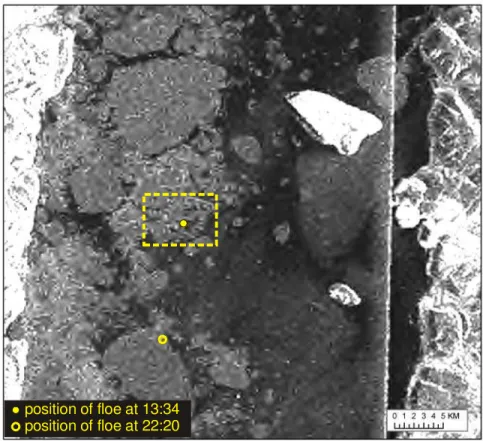
Floe N04 drifted south 12.1 km during the 8.77 hours that were spent sampling it, and moved at an average rate of 1.38 km/hr. Figure 16 shows the ScanSAR image that contains the 3.0 by 6.0 km floe (yellow box). The satellite image was acquired about one hour before the floe was sampled. Given the drift rate of 1.38 km/hr, the sampling area indicated by the solid yellow circle would have been about one kilometer further north when the image was acquired. The open circle shows the floe’s position when the field party departed.
position of floe at 13:34 position of floe at 22:20
Figure 16 ScanSAR image showing initial and final position of Floe N04, Nares Strait Floe sampled on 18 Aug, 13:34 to 22:20UTC Satellite image acquired on 18 August, 12:23UTC.
5.5 Floe N05
After the ice party returned from sampling Floe N04, Captain Vanthiel took advantage of the improved ice conditions on the Greenland side to travel to the northern part of Kennedy Channel. The objective of the trip was to download data from a shallow subsea mooring in Petermann Fjord. The ship departed for Petermann Fjord that evening, traveling through the night to arrive outside the fjord after breakfast on Sunday August 19. The oceanographic team spent the morning trying to retrieve data from their instrument in the fjord. In the afternoon, the ice party was given the option of sampling a floe, which the author eagerly accepted because sampling a multi-year ice floe this far north would likely be a once in a lifetime opportunity.
Since the ice party had been able to complete much more on Floe N04 with four people, Captain Vanthiel kindly agreed to spare two members from his crew for the on-ice work: one to function as bear monitor and another as an assistant. It was an arrangement that Captain Vanthiel took to joking about from here forward: “you want two of my crew?” The author and the bear monitor departed the ship at 12:56 and had landed on a floe at 13:09, just outside Polaris Bay (Figure 1). The floe was several kilometers across and had a well-established drainage network interconnecting the melt ponds (Figure 17). A total of 20 holes were mapped over the three transects shown in the aerial photograph in Figure 17-a. Transect 1 is also shown from the on-ice perspective in Figure 17-b.
The thickness of Floe N05 ranged from 2.70 to 8.63 m, with the thickest ice being on a ridge at the beginning of Transect 1 (Figure 18-b). The thinnest ice was measured at the edge of the drainage feature that terminated Transect 3. As with the previous four floes, the level ice surface did not reflect the variance that was observed in the bottom surface topography.
Having completed drill hole and EM measurements at 20 stations, a 3.6 m long core was retrieved from the 6.77 m thick ice at Flag 14 (Transect 2). The core was processed for the temperature and salinity measurements presented in Figure 19. Strength measurements were not conducted due to the limited amount of time that was available for sampling. The temperature of Floe N05 ranged from -1.4°C near the surface to a minimum of -3.5°C at a depth of 2.80 m. The salinity of the ice ranged from 0.1 to 2.9 ‰.
Measurements on Floe N05 were complete by 18:00 hours. The floe drifted 10.2 km south during the 5.1 hours that were spent sampling it, traveling at an average rate of 2.01 km/hr – faster than the four previous floes. With the field party safely back on the ship, Captain Vanthiel was eager to return to Nares Strait. He did not want the Henry Larsen being the only obstacle to impede the progress of the gigantic floes that were headed in his direction. One advantage of working in Nares Strait was that floes had already been slowed or split by the two natural islands north of it (Hans Island and Franklin Island).
Floe N05 was not captured in the satellite image for August 20 because it was much further north than the coverage extended.
20 18 19 14 15 11 4 5 6 7 8 9 10 16 17 3 1 2 12 13
a
b
Figure 17 Floe N05 (a) from the air and (b) level surface along the main transect. Floe N05 was several kilometers across. Circles in (a) show the locations of the three drill hole
transects, two of which are shown in (b).
Figure 18 Floe N05 (a) plan view of transects and (b) corresponding sail and keel profiles. The maximum measured thickness was 8.62 m.
-8 -6 -4 -2 0 2 4 -20-10 0 10 2030 4050 60 -120 -100 -80 -60 -40 -20 Ic e t h ic k n e s s , d ri ll h o le s ( m ) X dista nce (m ) Y dis tance (m ) Floe N05 Transect 1 Transect 2 Transect 3 -120 -100 -80 -60 -40 -20 0 20 -80 -60 -40 -20 0 20 40 60 80 X distance (m) Y di st anc e (m ) Transect 1 Transect 2 Transect 3 Floe N05
(a)
(b)
-5.5 -5.0 -4.5 -4.0 -3.5 -3.0 -2.5 -2.0 -1.5 -1.0 -0.5 0.0 -4 -3 -2 -1 0 1 2 3 4 Ice temperature (°C) and salinity (‰)
D ept h ( m ) temperature, N05 Flag 14 salinity, N05 Flag 14
Figure 19 Temperature and salinity profiles of Floe N05. Ice at Flag 14 was 6.77 m thick.
5.6 Floe N06
The ship was back on site in Nares Strait by Monday morning August 20. The oceanographic team spent that morning recovering oceanographic instrumentation, while the ice team devised a new instrument for measuring ice thickness (the old one had been damaged on Floe N05). By lunch, the author reported to the Captain that a new tool was successfully in hand and that the ice party could, with his permission, spend the afternoon sampling a sixth floe. He agreed, so after a quick lunch the ice party departed the ship. At 12:30 Floe N06 had been selected. Although the floe was only 500 m in diameter, the 3.5 to 4.0 m high ridge that crossed it promised very thick ice (Figure 20-a).
Three transects were mapped on Floe N06 but, in the interest of time, measurements were made along only two of them. Twenty holes were drilled on one side of the ridge, and one hole was drilled on the other side of the ridge (Figure 21-a). No measurements were made on the ridge crest itself. That would have been futile, given that the four metre high ridge would easily consume the 16 m of auger that was available. Instead, drilling commenced between the ridge crest and a drainage feature at the base of the ridge, on one side.
The measured thickness at that first station (Flag 1) was 7.63 m (Figure 21-b). The next station, Flag 2, was made in the 0.29 m deep drainage feature at the base of the ridge, where the ice was 11.21 m thick. The thickest ice was measured about 40 to 50 m from the ridge crest, at Flags 4 and 5, where the ice was more than 16 m thick (Figure 20-b). At 16 m, the ice was beyond the maximum drillable depth of the auger – all of the flights had been used, yet the bottom of the ice had not been penetrated. Most of the drill holes on Floe N06 were from 9 to 12 m thick, with the exception of a few holes near melt ponds, where the ice was 5.82 to 8.11 m thick. The hole that was drilled on the other side of the ridge had a thickness of 9.91 m and a freeboard of 1.50 m. There is some question about whether the actual ice bottom was measured at Flag 1 – or was the tape measure caught in a void? The ice was probably thicker than 7.63 m, given its freeboard of 1.29 m and the thickness of the neighboring ice.
5.6.1 Temperature and Salinity Profiles
Having completed the backbreaking work of drilling 21 holes in what was mostly 10 m thick ice, the team set upon retrieving a 5 m deep core from the ice at Flag 5, where the ice was more than 16 m thick. A little over one metre of ice had been drilled when the corer slowed, and became stuck. The power head was removed from the corer and many, many attempts were made to reverse the barrel out of the hole – to no avail. Realizing that the time was fast approaching for the helicopter pick-up, the ice party called the ship to request that the pilot bring out a chainsaw to help retrieve the barrel. The ship didn’t have one. So, the ice team used the 150 cm diameter auger to drill a necklace of holes around the barrel and then chisel it out. Two hours later, the barrel was finally free (Figure 22). Figure 23 shows the temperature and salinity profiles that were measured on the fragmented core from Flag 5. Temperatures in the uppermost metre of ice were near -1.0°C, although it is recognized that the temperature of the ice would have been affected by the two hour delay in processing the core. Salinities ranged from 0 to 0.3 ‰.
3 4 5 6 7
a
b
Figure 20 Floe N06 from the (a) air and (b) ice.
The floe was about 500 m in diameter and had a 3.5 to 4.0 m high ridge running across it. The yellow circle in (a) shows where satellite tracking beacon 47552 was installed on the floe. In
(b), the ice at Flags 4 and 5 was more than 16 m thick (see below).
Figure 21 Floe N06 (a) plan view of transects and (b) corresponding sail and keel profiles. Flags 4 and 5 are circled in (a) because that is where the auger could not fully penetrate what
appeared to be level ice – at more than 16 m thick, the ice was beyond the limit of the auger. -20 -15 -10 -5 0 5 0 10 20 30 40 50 -140 -120 -100 -80 -60 -40 -20 0 Ic e t h ic k n e s s , d ri ll h o le s ( m ) X dista nce (m ) Y dis tance (m) Floe N06 Transect 1 Transect 2 -140 -120 -100 -80 -60 -40 -20 0 20 -40 -20 0 20 40 60 80 100 120 X distance (m) Y dis tanc e (m) Transect 1 Transect 2 Floe N06
circled data markers indicate flags where 16 m auger did not penetrate bottom.
flag 4 flag 5 ridge
Figure 22 One happy man, after having labored to retrieve the corer for two hours! -5.5 -5.0 -4.5 -4.0 -3.5 -3.0 -2.5 -2.0 -1.5 -1.0 -0.5 0.0 -4 -3 -2 -1 0 1 2 3 4 Ice temperature (°C) and salinity (‰)
D ept h ( m ) temperature, N06 Flag 5 salinity, N06 Flag 5
Figure 23 Temperature and salinity profiles in the uppermost metre of ice at Floe N06. Ice at Flag 5 was more than 16 m thick.
5.6.2 Satellite View
The field party finally left Floe N06 at 17:30, after having spent a very long afternoon on the ice. During the 6.8 hours that were spent on the floe, it drifted 10.1 km south at an average rate of 1.49 km/hr. The red circles in Figure 24 show the trajectory that was mapped using a global positioning system during the time that the field party arrived on the floe, to when they left. The floe’s trajectory and the average drift rate were used to determine the approximate location of Floe N06 when the image was acquired, five hours before the field party arrived on the floe. The yellow box is drawn with a high degree of uncertainty first, because the floe was only about 500 m in diameter and second, because the image was acquired well before the floe was visited.
position of floe at 16:30 position of floe at 23:18
floe’s trajectory from 16:30 to 23:18
Figure 24 Standard image containing Floe N06, Nares Strait.
Floe sampled 20 August, 16:30 to 23:18UTC. Satellite image from 20 August, 11:25UTC.
5.6.3 Beacon Installation on Floe N06
Only an afternoon was spent on Floe N06, but an enormous amount of pain and effort went into sampling that floe – the thickest ice that the author had been on to date. Several drill flights had to be abandoned because the drill team could not afford to spend more than about 20 minutes trying to retrieve them: measuring the ice thickness elsewhere on the floe was a higher priority. The corer had gotten stuck but, mercifully, it had been retrieved. Both the coring unit and a number of drill flights had sustained damage from the beating that Floe N06 had given them.
It was decided that Floe N06 should be the home for one, of the two satellite tracking beacons that the Canadian Ice Service (CIS) had provided for tracking multi-year ice. Mapping the movement of multi-year is an area that the author and CIS have collaborated on for many years. In fact, one of the multi-year ice floes on which a satellite tracking beacon was installed during the 2006 Nares Strait field program traveled from Kane Basin to the coast of Newfoundland, a distance of more than 3000 km, in just over nine months. It was hoped that the beacon that was installed on Floe N06 would survive its journey south, to yield several months of data on the floe’s trajectory.
Normally, the beacons are placed on the highest point of a floe, but beacon 47552 was installed on small ice hummock within a fairly level area of Floe N06 (Figure 13-a). The beacon was installed somewhere other than the ridge crest with the intention of determining whether a good part of the floe survives the transit south, or merely a remnant of the ridge. Drill hole measurements indicated that the ice in that region was over 10 m thick.
As it turned out, Floe N06 was not a winner. It traveled south for several months and then stopped transmitting when it was along the coast of Baffin Island. Either it stopped transmitting because a bear sabotaged it or because it was swamped with water (as the floe disintegrated). Since experience has shown that the beacons are pretty much bear-proof, one could conclude that the 500 m diameter floe was too small to survive the trip south.
5.7 Floe N07
Since Floe N06 had damaged the corer and drill rods on Monday August 20, the following day was spent repairing and refurbishing equipment. That gave the ice party a much-needed day off (the ice). On Wednesday August 22, the Captain offered the opportunity to sample a seventh floe, for the entire day. Having the whole day to conduct measurements was a blessing, because trying to characterize a floe in an afternoon was extremely difficult. Both Floes N05 and N06 had been sampled in an afternoon.
Up to that point, most of the sampled floes in Nares Strait had been near the edge of the pack ice along the Ellesmere Coast. It was also of interest to venture into the interior of the moving pack, closer to shore. The field party departed the ship at 8:50 and had selected a floe by 9:06, about 2 km from the Ellesmere Island. Floe N07 was a small floe by any standard – 500 m long and only 250 m wide – but it was larger than the surrounding ice floes. A large drainage feature extended along the centre of the floe, nearly spanning one end, to the other (Figure 26-a). A total of 30 holes were drilled over five transects on Floe N07. The ice surface along the transect in Figure 26-b shows that Floe N07 had the characteristic undulations of multi-year ice. The floe thickness ranged from 2.12 to 8.40 m, with freeboards of 0.15 to 1.86 m (Figure 27-b).
5.7.1 Temperature, Salinity and Strength Profiles
Floe N07 was the first floe on which the full suite of measurements was made: thickness, temperature, salinity and strength. A 5.0 m long core was retrieved from the 6.60 m thick ice at Flag 4, the location of which is shown in Figure 26-a. Figure 28 shows the temperature, salinity and strength profiles of the ice at Flag 4. Temperatures in the uppermost 1.0 m were consistently about -1.1°C. There was a noticeable decrease in temperature between depths 1.0 to 1.2 m. That decrease coincided with the 1.0 m freeboard – ice above the waterline was warmer than below it. The coldest temperatures occurred below the 2.0 m depth, where the ice temperatures were -3.0 to -3.5°C. The ice salinity ranged from 0 to 2.1 ‰. As expected, the least saline ice occurred in the uppermost metre of ice.
Once the cores had been removed from the ice and processed, the NRCC borehole indentor was used to conduct strength tests in the 150 mm diameter borehole. A description of the borehole indentor is given in Appendix B. The strengths that are presented in Figure 26-b are the maximum ice pressures that were observed during a test. The integrity of the ice determined the speed at which the indentors penetrated the ice. In this report, no attempt was made to compensate test results from the different depths for the rate effect, as was done for first-year ice in Johnston et al. (2003). The rate-compensated strengths will be published elsewhere. The maximum strength of Floe N07 at the different test depths ranged from 11.5 to 21.5 MPa. The lowest strengths were measured in the uppermost 0.60 m of ice.