Algorithms and inference for simultaneous-event multivariate point-process, with applications to neural data

Algorithms and Inference for Simultaneous-Event

Multivariate Point-Process, with Applications to

Neural Data

by

Demba Ba

"^*S^AC _{geS SINTITUTE} OF TECHNOLOGY

JUN 17 2011

LIBRARIES

Submitted to the Department of Electrical Engineering and Computer

Science

in partial fulfillment of the requirements for the degree of

Doctor of Philosophy in Electrical Engineering

at the

MASSACHUSETTS INSTITUTE OF TECHNOLOGY

ARCHNES

June 2011

©

Massachusetts Institute of Technology 2011. All rights reserved.

A uthor ...

...

.

Department ot Electrical Engineering and Computer Science

May 19, 2011

Certified '

LI/

_{Emery N. Brown}

Professor of Computational Neuroscience

and Professor of Health Sciences and Technology.

Thesis Supervisor

Accepted by ...

L

0 ULeslie A. Kolodziejski

Algorithms and Inference for Simultaneous-Event

Multivariate Point-Process, with Applications to Neural

Data

by

Demba Ba

Submitted to the Department of Electrical Engineering and Computer Science on May 19, 2011, in partial fulfillment of the

requirements for the degree of

Doctor of Philosophy in Electrical Engineering

Abstract

The formulation of multivariate point-process (MPP) models based on the Jacod like-lihood does not allow for simultaneous occurrence of events at an arbitrarily small time resolution. In this thesis, we introduce two versatile representations of a simultaneous-event multivariate point-process (SEMPP) model to correct this important limitation. The first one maps an SEMPP into a higher-dimensional multivariate point-process with no simultaneities, and is accordingly termed the disjoint representation. The second one is a marked point-process representation of an SEMPP, which leads to new thinning and time-rescaling algorithms for simulating an SEMPP stochastic process. Starting from the likelihood of a discrete-time form of the disjoint representation, we present derivations of the continuous likelihoods of the disjoint and MkPP represen-tations of SEMPPs.

For static inference, we propose a parametrization of the likelihood of the disjoint representation in discrete-time which gives a multinomial generalized linear model (mGLM) algorithm for model fitting. For dynamic inference, we derive generalizations of point-process adaptive filters. The MPP time-rescaling theorem can be used to assess model goodness-of-fit.

We illustrate the features of our SEMPP model by simulating SEMPP data and by analyzing neural spiking activity from pairs of simultaneously-recorded rat thala-mic neurons stimulated by periodic whisker deflections. The SEMPP model demon-strates a strong effect of whisker motion on simultaneous spiking activity at the one millisecond time scale. Together, the MkPP representation of the SEMPP model, the mGLM and the MPP time-rescaling theorem offer a theoretically sound, practical tool for measuring joint spiking propensity in a neuronal ensemble.

Thesis Supervisor: Emery N. Brown

Title: Professor of Computational Neuroscience and Professor of Health Sciences and Technology.

Acknowledgments

"How does it feel?", "What's next?". Obviously, many have asked me these questions. This is not the appropriate place to answer the second question. However, I will try to answer the second one in a few sentences.

I have mixed feelings about my experience as a graduate student. I, as the ma-jority of grad students, had to battle with many of the systemic idiosyncrasies of grad school and academia. A shift occurred in my way of thinking when it became obvious that the said idiosyncrasies were taking a toll on my experience as a graduate student. I told myself that I would make my PhD experience what I wanted to be. That is precisely what I did after my M.S.I thought about the best way of satisfying graduation requirements while building an academic profile that reflected my own view of science/knowledge/research. I followed that approach and, simply because of this, I am happy with wherever it has led me, as a thinker, as an academic, as a researcher.

A number of people have helped me to achieve this objective. First, I would like to thank my thesis supervisor Emery Brown, who picked me up at a time when I was having a difficult time transitioning from M.S. to PhD. For his moral support and trust, and a number of other reasons, I am forever grateful. I would also like to thank George Verghese who has consistently given me moral support since the 2004 visit day at MIT when he saw me in a corner and said "Don't be shy, you should mingle and talk to people...". I would also like to thank professor Terry Orlando for his moral and financial support during the transition period between M.S. and PhD. Many thanks to professor John Tsitsiklis for agreeing to serve on my thesis committee, as well as professor Sanjoy Mitter.

I would like to thank my family for their support during these arduous years. My mom Fama, my dad Bocar, my sister and brothers: Famani, Khalidou, Moussa and Moctar. The latter two's sons and daughters also deserve mention here: let's talk if and when you have to decide between Harvard and MIT. I would also like to thank my cousin Elimane Kamara, my aunt Gogo Aissata, Rose, my aunt Tata Rouguy and

her husband Tonton Hamat.

I would like to thank my friends. My first contact with MIT was through Zahi Karam, who told me to go to Georgia Tech instead. (Un)fortunately, Tech didn't accept me. Alaa Kharbouch, Hanan Karam, Akram Sadek, Mack Durham, Najim Dehak, Yusef Asaf, Valerie Loehr, Yusef Mestari, thanks for the good times and the moral support. Borjan Gagoski is the first of my cohorts that I met: we've been through the tough years together. Among cohorts, I'd also like to thank Faisal Kashif, Bill Richoux and Jennifer Roberts (correction, Jen and I went to University of Maryland College Park together.. .sorry Borjan). Also at MIT, I would like to thank Sourav Dey and his wife (Pallabi), Obrad and Danilo Scepanovic, Miriam Makhlouf (This Is Africa, TIA, represent!), Hoda Eydgahi, Camilo Lamus, Antonio Molins, Ammar Ammar, Yi Cai, Paul Azunre, Paul Njoroge (African man!) and Ali Motamedi. I would also like to thank Siragan Gailus, Sangmin Oh, Sangyun Kim, Nevin Raj, Subok Lee, Caroline Lahoud, Antonio Marzo and Shivani Rao.

Through my time at MIT, I have interacted with certain members of the MIT staff, who I cannot forget to acknowledge: Lourenco Pires, Debb of MTL, Lisa Bella, Sukru Cinar and Pierre of custodial services.

Special thanks to the people who helped me to get industry experience at MSR and Google, and coached me through those experiences: Rico Malvar, Dinei Florencio, Phil Chou (all three of MSR), Kevin Yu and Xinyi Zhang, both of Google. It has been a pleasure interacting with you and meeting you. I have also made friends through these internships, notably Flavio Ribeiro at MSR, Lauro Costa and Shivani Rao at Google.

Many thanks to my friends from back home: Lahad Fall, Fatou Diagne, Suzane Diop, Wahab Diop and their family, Pape Sylla, Babacar Diop and Amadou Racine Ly. I would also like to thank my high-school friend Said Pitroipa.

I would like to thank professors Staffilani and Melrose of the MIT math department for being excellent teachers, and inspiring me.

Last but not least, I would like to thank current and ex members of the Brown Lab for bearing with me, notably Sage, Hideaki, Neal and Deriba.

Contents

1 Background, Introduction and Scope 15

1.1 Introduction . . . . 15

1.2 Background . . . . 16

1.2.1 Non-likelihood methods . . . . 16

1.2.2 Likelihood methods . . . . 17

1.3 Contributions . . . . 18

2 Discrete-Time and Continuous-Time Likelihoods of SEMPPs 21 2.1 Simultaneous-event Multivariate Point Process . . . . 21

2.2 The disjoint and marked point-process representations . . . . 22

2.2.1 The disjoint representation . . . . 22

2.2.2 The marked point-process representation . . . . 24

2.3 Likelihoods . . . . 26

2.3.1 Discrete-time likelihood . . . . 26

2.3.2 Continuous-time likelihoods . . . . 27

3 Rescaling SEMPPs 31 3.1 Rescaling uni-variate point processes . . . . 31

3.2 Rescaling multivariate point processes . . . . 33

3.3 Application to simulation of SEMPPs . . . . 34

3.3.1 Algorithms based on the time-rescaling theorem . . . . 34

3.3.2 Thinning-based algorithms . . . . 36

3.4 Application to goodness-of-fit assessment . . . .

4 Static and Dynamic Inference

4.1 Static m odeling . . . . 4.1.1 Generalized linear model of the DT likelihood . . . . 4.1.2 Maximum likelihood estimation . . . . 4.1.3 Numerical examples of savings due to linear CG . . . . 4.2 Dynamic modeling: SEMPP adaptive filters . . . . 4.2.1 Adaptive filters based on approximate discrete-time likelihood 4.2.2 Adaptive filters based on exact discrete-time likelihood

(multi-nom ial filters) . . . .

5 Data Analysis

5.1 Thalamic firing synchrony in rodents . . . .

5.2 Experim ent . . . . 5.3 Statistical model . . . . 5.3.1 Measures of thalamic firing synchrony . . . . 5.4 R esults . . . . 5.4.1 Results for individual pairs . . . . 5.4.2 Summarizing results of analyses on all pairs . . . 5.5 Decoding examples . . . . 5.5.1 Decoding results on real data . . . . 5.5.2 Decoding results on simulated data . . . . 5.6 Summary of findings . . . .

6 Conclusion

6.1 Concluding remarks. . . . . 6.2 O utlook . . . . 6.2.1 Modeling stimulus noise . . . . 6.2.2 Dimensionality reduction . . . . 6.2.3 Large-scale decoding examples using simultaneous

61 61 62 64 65 . . . . 68 . . . . 68 . . . . 70 . . . . 72 . . . . 73 . . . . 75 . . . . 94 99 . . . . 99 . . . . 101 . . . . 101 . . . . 101 events . . . 102

6.2.4 Adaptive filtering for the exponential family . . . . 102

A Chapter 1 Derivations 105

A.1 Derivation of the Ground Intensity and the Mark pmf . . . . 105 A.2 Expressing the Discrete-time Likelihood of Eq. 2.12 in Terms of a

Dis-crete Form of the MkPP Representation . . . . 106

B Gradient vector and Hessian matrix of multinomial GLM log-likelihood107

C Second-order statistics of a multinomially-distributed random

List of Figures

3-1 Standard raster plots of the simulated spiking activity of each neuron in a triplet in response to a periodic whisker deflection of velocity

v = 50 m m /s. . . . . 39 3-2 New raster plots of non-simultaneous ('100', '010' and '001') and

si-multaneous ('110', '011', '101' and '111') spiking events for the three simulated neurons of in Fig. 3-1. . . . . 41

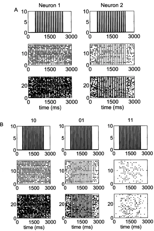
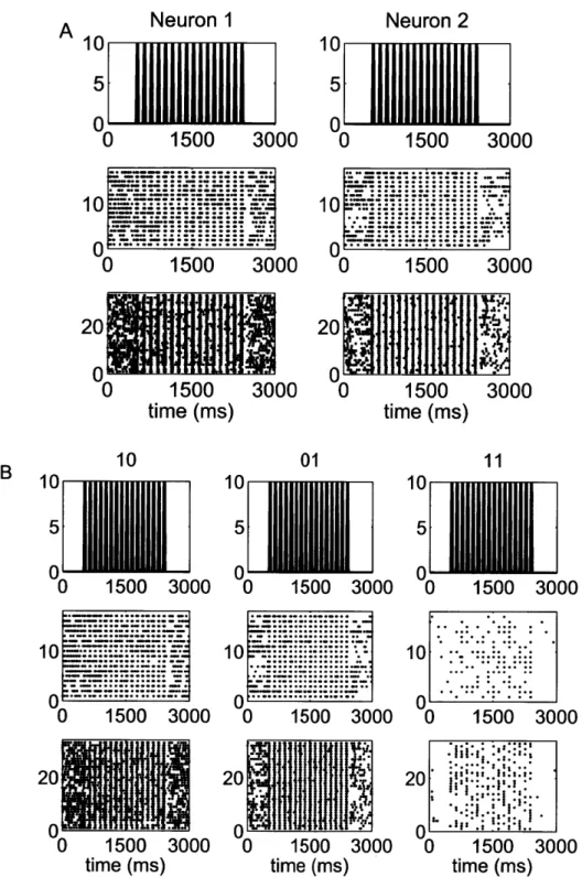
5-1 Raster plots of the spiking activity of a representative pair of neurons in response to a periodic whisker deflection of velocity v = 80 mm/s. 77

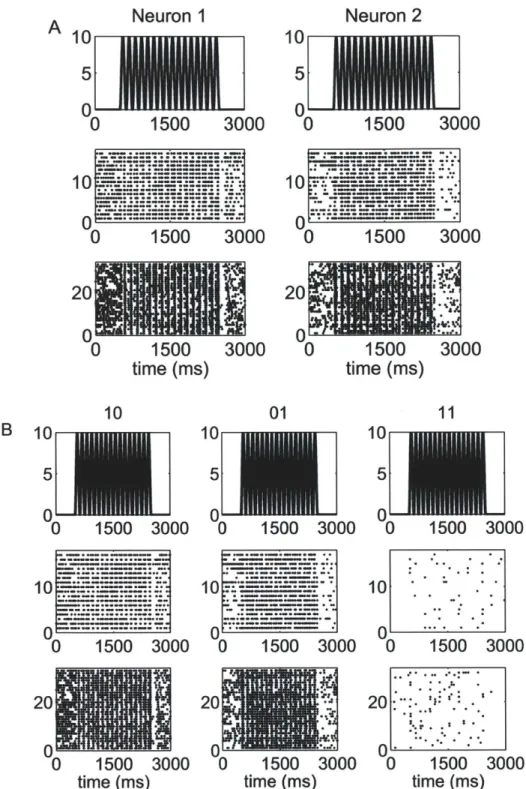
5-2 Raster plots of the spiking activity of a representative pair of neurons in response to a periodic whisker deflection of velocity v = 50 mm/s. 78 5-3 Raster plots of the spiking activity of a representative pair of neurons

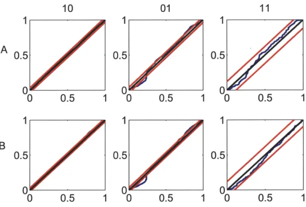
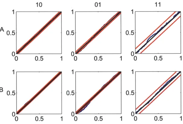
in response to a periodic whisker deflection of velocity v = 16 mm/s. 79 5-4 Goodness-of-fit assessment by KS plots based on the time-rescaling

theorem for the pair in Fig. 5-1. . . . . 80 5-5 Goodness-of-fit assessment by KS plots based on the time-rescaling

theorem for the pair in Fig. 5-2. . . . . 81 5-6 Goodness-of-fit assessment by KS plots based on the time-rescaling

theorem for the pair in Fig. 5-3. . . . . 82 5-7 Comparison of the modulation of non-simultaneous and simultaneous

events for each stimulus velocity. . . . . 83 5-8 Comparison of the modulation of the simultaneous '11' event across

5-9 Comparison of zero-lag correlation over the first and last stimulus cy-cles, for each stimulus velocity. . . . . 85 5-10 Comparison of zero-lag correlation across stimuli over the first and last

stim ulus cycles. . . . . 86 5-11 Effect of the history of each neuron in the pair on its own firing and

on the other neuron's firing. . . . . 87 5-12 Population comparison of the modulation of non-simultaneous and

si-multaneous events for each stimulus velocity. . . . . 88 5-13 Empirical distribution of the time of occurrence of maximum stimulus

modulation with respect to stimulus onset for all 17 pairs in the data set... ... 89 5-14 Population comparison of the modulation of the simultaneous '11'

event across stim uli. . . . . 90 5-15 Population comparison of zero-lag correlation over the first and last

stim ulus cycles. . . . . 91 5-16 Population comparison of zero-lag correlation across stimuli over the

first and last stimulus cycles. . . . . 92 5-17 Population summary of each neuron's effect on its own firing and on

the other neuron's firing. . . . . 93 5-18 Decoded low-velocity stimulus using independent and joint decoding. 94 5-19 Decoded low-velocity stimulus during first and last cycles, and averaged

across cycles. . . . . 95 5-20 Comparison, for each stimulus, of administered stimulus to

jointly-decoded stimulus using real data. . . . . 96 5-21 Comparison, across stimuli, of administered stimulus to jointly-decoded

stimulus using real data. . . . . 97 5-22 Comparison, across stimuli, of administered stimulus to jointly-decoded

stimulus using simulated data. . . . . 98 5-23 Comparison, for each stimulus, of administered stimulus to

List of Tables

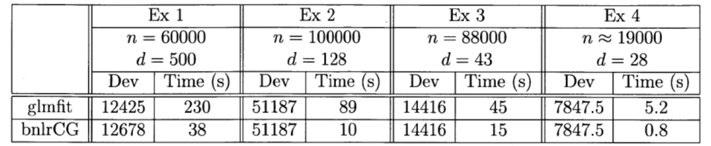
2.1 Map from dN(t) to dN*(t), C = 3, M = 8 ... 24 4.1 Comparison of gImfit and bnlrCG on various neuroscience data sets . 52

Chapter 1

Background, Introduction and Scope

1.1 Introduction

Neuroscientists explore how the brain works by applying sensory stimuli and record-ing the responses of neurons. Their goal is to understand the respective contributions of the stimulus, as opposed to the neurons' intrinsic dynamics, to the observed activ-ity. Nowadays, it is not uncommon to record simultaneously from multiple neurons. However, techniques for the sound analysis of data generated by such experiments have been lagging a step behind.

Motivated mainly by applications in neuroscience, the aim of this thesis is to develop a generic framework for the rigorous analysis of multivariate-point-process phenomena. Perhaps it is easier to understand the scope of this thesis by dissecting its title. Loosely, a uni-variate point process is a sequence of discrete events (e.g. firing of a neuron, arrival of a bus/passenger at a station) that occur at random points in continuous time (or space). In general, there could be multiple such processes evolving in parallel, in which case we speak of a multivariate point-process. Effectively, a multivariate point process is a finite-dimensional vector process, the components of which are uni-variate point processes. In the literature, significant attention has been given to the particular case of multivariate point processes for which the probability of

simultaneous events/arrivals in any pair of components is negligible. Meanwhile, the

case where simultaneous arrivals/events in multiple components cannot be ignored has received little to no attention. From a theoretical standpoint, this latter fact is the main motivation of this thesis.

For data analysis tasks, this thesis develops algorithms for simulation and estima-tion of simultaneous-event multivariate point-process models. In practice, the type of inference/estimation problems we would like to solve fall within the class of para-metric density estimation problems. We call such problems 'static' if the parameters of the model are fixed. If one allows the parameters of the model to vary (e.g. with time), then we call such models 'dynamic'. We demonstrate the efficacy of the infer-ence and simulation algorithms on neural data. These data consist of spiking activity from simultaneously-recorded rat thalamic neurons stimulated by periodic whisker deflections.

1.2 Background

Existing techniques to analyze neural data fall mainly into two categories: likelihood methods and those that do not make strong assumptions, if any, about the generating process of the data. We term the latter non-likelihood methods.

1.2.1 Non-likelihood methods

As a class, non-likelihood based methods are limited due to their inability to quantify the extent to which the stimulus, as opposed to spiking history, modulates the joint activity of a group of neurons. The cross-correlogram and the cross-intensity function are two similar approaches which reduce the problem of analyzing ensemble neural data to one of characterizing the relationships between pairs of neurons. Given a pair of neural spike trains and a fixed bin width, the un-normalized cross-correlogram [8] is the deterministic cross-covariance between the two spike trains, computed at a series of lags. An underlying assumption of this method is that of stationarity, which loosely states that the joint statistics of the pair of neurons do not change over time. Although convenient, such an assumption is hard to justify given how plastic neural systems are. The cross-intensity function [6] estimates the rate of a given neuron at different lags relative to another neuron. In spite of its simplicity, the cross-intensity function has not gained as much popularity as the cross-correlogram within

the neuroscience community. The joint peri-stimulus time histogram (JPSTH) [17] is another histogram-based method which operates on pairs of neurons. The JPSTH is the natural extension to pairs of neurons of the well-known PSTH: it is a two-dimensional histogram displaying the joint spike count per unit time at each time u for the first neuron and time v for the second neuron. The JPSTH addresses one of the drawbacks of the cross-correlogram, which is the stationarity assumption within trials. However, due to its reliance on a stationarity assumption across trials, the JPSTH may lead to incorrect conclusions when there exists across-trial dynamics. In [45], the authors incorporate a statistical model for time-varying joint-spiking activity within the JPSTH framework. They show that this allows for more efficient computation of the joint-firing rate of pairs of neurons. Among non-likelihood methods, spike pattern classification techniques allow one to analyze associations beyond pairwise ones. These methods can be used to assess the statistical significance of certain spike patterns among multiple neurons [1, 18, 19, 34]. One of the challenges posed by spike pattern classification is that of selecting the appropriate pattern size.

1.2.2 Likelihood methods

Likelihood methods are closest in spirit to the framework we propose in this thesis. Among such methods, there are those based on information geometry [3, 31] and those based on point processes [24, 33]. Likelihood methods based on information geometry rely on an expansion of the log of the joint pmf of a vector binary process as a linear combination of its moments. Recently, a method was proposed which combines information geometry and adaptive filtering to track the evolution over time of the moments of a vector binary process [39]. The nature of experiments in neuroscience is such that it is natural to expect the joint statistics of single neurons or of an ensemble to vary with time. In [39], the authors use a stochastic continuity constraint on the moments in order to recover the time-varying nature of the statistics of the data. One would expect, however, that the stimulus and/or spiking history of neurons in an ensemble would encode information about the time-varying nature of the joint statistics of the ensemble. This is precisely what point-process methods 17

attempt to do. Building on their success in characterizing single-neuron data [43], point-process methods have been shown to provide a sensible framework within which one is able to isolate the contributions of stimulus as opposed to history to the joint activity of a group of neurons [33]. However, there is a caveat: the assumption that, for small enough time resolution, the probability of joint firing among any two or more neurons in the ensemble is negligible. As the time resolution becomes arbitrarily small, this leads to the Jacod likelihood for multivariate point processes with no simultaneities [22, 14]. The Jacod likelihood is expressed as the product of univariate point-process likelihoods.

1.3 Contributions

Likelihood methods based on point processes assume that either the components of the multivariate point process are independent, or that simultaneous occurrences of events in any two components can be neglected. These assumptions turn out to be convenient as, in both cases, one can fit an approximate model to the multivariate point process by performing inference separately on each of its components. The case where the probability of simultaneous occurrences cannot be neglected has received little to no attention in the literature. Ventura et al. [45] developed a likelihood procedure to overcome this limitation for analyzing a pair of neurons. In [25], Kass et al. extend Ventura's approach to multiple neurons. Solo [41] recently reported a simultaneous event multivariate point-process (SEMPP) model to correct this im-portant limitation. However, in his treatment, Solo does not provide a framework for inference based on real data. Here, we propose a quite general framework for inference based on SEMPP observations. We introduce two representations of an SEMPP. The so-called disjoint representation transforms an SEMPP into an auxil-iary multivariate point-process with no simultaneities. The multivariate point-process theorem [14] can be applied to this new representation to assess model goodness-of-fit. The marked point-process (MkPP) representation [14] leads to algorithms for simulating an SEMPP stochastic process. In discrete-time (DT), the likelihood of

the disjoint representation can be expressed as a product of conditional multinomial trials (rolls of a dice). Starting from such an approximation, we derive the limiting continuous-time likelihood, i.e. that of the continuous-time (CT) disjoint representa-tion. We also derive a form of this likelihood in terms of the MkPP representarepresenta-tion. In practice, model fitting is performed in discrete-time. We propose a parametrization of the likelihood of the disjoint process in discrete-time which turns it into a multivariate generalized linear model (mGLM) with multinomial observations and logit link [16]. We propose and make available a very efficient implementation of the mGLM, which is up to an order of magnitude faster than standard implementations, such as Mat-lab's. Last but not least, we derive natural generalizations of point-process adaptive filters that are able to handle simultaneous occurrences of events in multivariate point processes.

We apply our methods to the analysis of data recorded from pairs of neurons in the rat thalamus in response to periodic whisker deflections varying in velocity. Our model provides a direct estimate of the magnitude of simultaneous spiking propensity and the degree to which whisker stimulation modulates this propensity.

Chapter 2

Discrete-Time and Continuous-Time

Likelihoods of SEMPPs

In this chapter, we begin with a simple definition of an SEMPP. Then, We show an ex-plicit one-to-one mapping of an SEMPP to an auxiliary MPP with no simualteneities, albeit in a higher dimensional space. We call this new MPP the disjoint representa-tion. The disjoint representation admits an alternate equivalent representation as an MkPP with finite mark space, which we also develop here. Last, we derive discrete-time and continuous-discrete-time SEMPP likelihoods. In discrete-discrete-time, the likelihood of the disjoint representation can be expressed as a product of conditional multinomial tri-als. Starting from this likelihood, we derive the continuous-time likelihood of the disjoint process by taking limits. We also derive a form of the continuous-time likeli-hood in terms of the MkPP representation. The Jacod and univariate point-process likelihoods are special cases of the continuous-time likelihoods obtained here.

We walk the reader through all key derivations. The less essential derivations are shown in one of the appendices.

2.1 Simultaneous-event Multivariate Point Process

We consider an observation interval (0, T] and, for t E (0, T], let N(t) = (N1(t), N2(t),- , Nc(t))'

be a C-variate point-process defined as Nc(t) =

fo

indica-tor function which is 1 if there is an event at time t and 0 otherwise, for c = 1, -- -, C.

that each component c has a conditional intensity function (CIF) defined as

Ac(t|Ht) = lim P[N,(t + A) Nc(t) 11Ht] (2.1)

where Ht is the history of the C-variate point process up to time t. Let dN(t) =

(dN1(t), dN2(t), ... , dNc(t))' be the vector of indicator functions dNc(t) at time t.

We may treat dN(t) as a C-bit binary number. Therefore, there are 2c possible outcomes of dN(t) at any t. C of these outcomes have only one non-zero bit (that is, only one event in one component of dN(t)) and 2c-C-1 have two or more non-zero bits. That is, there is an event at time t in at least 2 components of dN(t). The last

outcome is dN(t) = (0, ... , 0)'.

We define N(t) as a simultaneous-event multivariate point process (SEMPP) if, at any time t, dN(t) has at least two non-zero bits. That is, events are observed simultaneously in at least two of the components of N(t). The special case in which, at any t, dN(t) can only take as values one of the C outcomes for which only one of the bits of dN(t) is non-zero is the multivariate point process defined by Vere-Jones [14]. The joint probability density of N(t) in this special case is given by the Jacod likelihood function [32], [24, 14].

2.2 The disjoint and marked point-process representations

We introduce the disjoint representation, which maps an SEMPP into an auxilliary MPP with no simultaneities, in a higher dimensional space. This new disjoint MPP admits an alternate representation as marked point-process with finite mark space.

2.2.1 The disjoint representation

To derive the joint probability density function of an SEMPP, we develop an alterna-tive representation of N(t). Let M = 20 be the number of possible outcomes of dN(t) at t. We define a new M- 1-variate point process N*(t) = (N*(t), N*(t), ... , N -1(t))'

of disjoint outcomes of N(t). That is, each component of N*(t) is a counting process for one and only one of the 2c-1 outcomes of dN(t) (patterns of C bits) that have

at least one non-zero bit. For any t, the vector dN*(t) = (dN*(t), - - - , dN _l (t))'

is an M-1-bit binary number with at most one non-zero bit. The non-zero element of dN* (t) (if any) is an indicator of the pattern dN(t) of C bits which occurs at t.

dN*(t) = (0, ... , 0)' corresponds to dN(t) = (0, ... , 0)'. We define the CIF of N* (t)

as

A*(t|Ht) = lim P[N7jt + A) -,Nm(t) = lIHt] (2.2)

where the counting process is N* (t) =

fo'

or representation.

One simple way to map from dN(t) to dN*(t) is to treat the former as a C-bit binary number, reverse the order of its bits, and convert the resulting binary number to a decimal number. We use this decimal number as the index of the non-zero component of dN*(t). The inverse map proceeds by finding the index of the non-zero entry of dN*(t), expressing this index as a C-bit binary number, and reversing the order of the bits to obtain dN(t). This one-to-one map is described in detail in the next few pages for the arbitrary C-variate case. First, we illustrate this one-to-one map in Table 2.1 for the case C = 3 and M = 8. In this example, N(t) is related to

N*(t) by

N1(t) = N*(t)+N*(t)+N*(t)+N*(t) (2.3)

N2(t) = N*(t) + N*(t) + N*(t) +N*(t) (2.4)

N2(t) = N*(t) + N*(t) + N*(t) +N*(t). (2.5)

The CIFs of N(t) are related to those of N*(t) in a similar fashion.

From N(t) to N*(t): For each t E (0, T], the vector dN(t) = (dN1(t), ... ,dNc(t))'

of counting measure increments of N(t) has entries either 0 or 1. Therefore, we can treat dN(t) as a C-length binary number. We let mdN(t) Ecl dNc(t)2c-1 be thei

decimal (base-10) representation of dN(t): mdN(t) E {0,... - 1 .

Table 2.1. Map from dN(t) to dN*(t), C = 3, M = 8 dN(t)' m dN*(t)' (1,0,0) 1 (1,0,0,0,0,0,0) (0,1,0) 2 (0,1,0,0,0,0,0) (1,1,0) 3 (0,0,1,0,0,0,0) (0,0,1) 4 (0,0,0,1,0,0,0) (1,0,1) 5 (0,0,0,0,1,0,0) (0,1,1) 6 (0,0,0,0,0,1,0) (1,1,1) 7 (0,0,0,0,0,0,1)

0, we let dN*(t) = (0, - --, 0)'. Otherwise, we let dN* (t) = 1 if m = mdN(t) and dNm(t) 0 otherwise. In this case, dN*(t) is an indicator vector for the event dN(t) which oc-curs at t. If we let N,(t) =

f'

a multivariate point-process of disjoint events from N(t).

From N*(t) to N(t): For each t E (0, T], the vector dN*(t) = (dN*(t),--- , dN2*c_1(t))'

is either (0, --- , 0)' or an indicator vector. In the former case, we let dN(t) =

(0, - --, 0)'. In the latter case, we would like to determine the event dN(t) that dN*(t)

is an indicator of. Let m c {1, ... ,2 - _{1} be the index of the non-zero entry of}

dN*(t) and bm = bmibm2 ... bmnc be the binary representation of m. If we let dN(t) =

(bmc, ... , bn2, bmi)', we obtain the event dN(t) that dN*(t) is an indicator of. Letting Nc(t) =

fS

We give the following definition, adapted from [14], of a marked point process on the real line.

Definition: A marked point process with locations on the real line R and marks in the complete separable metric space

M,

{(te,

{ti}

In-tuitively, one may think of an MkPP as follows: (a) events occur at random points in continuous-time (or space) according to the ground process, (b) every time an event occurs, one assigns a mark to this event by drawing a sample from a distribution which may very well depend on time, as well as the history of the ground process and/or past marks.

If we let 0 < ti < t2 < ... < tL < T denote the times in the observation interval (0, T] at which dN(t) has at least one non-zero bit, then we can express the disjoint process N*(t) as a marked point process (MkPP) {(tj, dN*(t,)}I_1 with M-1-dimensional mark space. At te, at least one of the bits of dN(t) is non-zero. The unmarked process {te}L_1 is the ground point process [14]. The mark, which is the index me of the non-zero bit of dN* (te) then indicates, through the map described above, exactly which of the M-1 patterns of C bits (outcomes of dN(t) other than (0, ... , 0)') occurred at te. At any other t, dN(t) = (0, ... , 0)'.

We denote by dN9(t) the indicator function that is 1 at te, E = 1,--- , L and zero at

any other t. The ground point process defines the times of occurrence of any pattern of C bits (outcomes of dN(t)) that are not all zero. For each m, the times at which

dN,*(t) is non-zero define the times of occurrence of one specific pattern of C bits

that are not all zero. It follows that the counting process and the CIF of the ground point process are respectively

M-1 Nq (t ) =

(

(

The probability of the marks is given by the multinomial probability mass function

A* (t|IHt)

P[dN*(t)= 1dNg(t) 1,Ht] = mI , (2.8)

A*(t|Ht)

for m = 1, ... , M-1. The derivations for Eqs. 2.7 and 2.8 are in Appendix A. The

event occurring in (0, T] is governed by the CIF A* (t|Ht) of the ground point process. When an event is observed in dNg(t), the marks are drawn from an M-1-dimensional history-dependent multinomial distribution (Eq. 2.8) to produce the corresponding event in N*(t), or equivalently N(t).

N.B: The careful reader will notice that I am being a bit cavalier when using the notation dN* (te): this is the indicator vector, the index of the nonzero entry of which is mt. For any te, E = 1, - --, L, dN*(tj) is automatically an indicator vector. For

any other t $ te, dN* (t) is the zero vector. So, in short, dN* (te) and its non-zero

index are two ways of representing the mark. I struggled with how to deal with the notation. In the end, this made the most sense. Hopefully, this does not cause too much confusion.

2.3 Likelihoods

Our goal is to derive the joint probability density function (PDF) of an SEMPP in discrete and continuous-time using straightforward heuristic arguments. We start with the likelihood for a discrete-time form of the disjoint representations and obtain continuous-time likelihoods by taking limits.

2.3.1 Discrete-time likelihood

To derive the joint PDF of N*(t) in discrete time, we define the discrete-time repre-sentations of N(t) and N*(t).

Choose I large and partition the interval (0, T] into sub-intervals of width A =

I- 1T. In discrete-time Nc(t) and N,(t) are respectively N,, = Nc(iA), N* i = N* (iA) for i 1, ... ,I. Let ANc,i = Nc Nc,i_1, and AN** = N,i - N* _.

Letting AN = (AN₁,i, - -, ANc,)', we choose I large enough so that ANci is 0 or

1. Either ANi (AN*', - -- , AN 4 _,)' has one event in exactly one component

or ANi* = (0,-- , 0)'. Let AN* = (AN*, -- - , AN*)' be the I x M-1 matrix of discretized outcomes for the observation interval (0, T]. Each ANi*, where i is the discrete-time index, is a realization from a multinomial trial with M outcomes (roll

of an M-sided die): M-1

P[AN,*lH,] =7

(A* [ilHi]A)AN*,i (1 - A*[ilHi]A)1 ANg,

where ANg, = Ng,i - Ng,i_1 = EM__AN* i N,, = Ng(iA). The probability mass

function of AN* can be written as the product of conditional M-nomial trial:

I

P[AN*] = P[ANi*Hi] + o(AL)

- A*[ilHi]A) 1-ANg,i + O(AL).

(2.11)

(2.12)

I M-1

i=1 m=1

We note that Eq. 2.12 can also be expressed in terms of a discrete-time form of the MkPP representation A.13. The manipulations are detailed in Appendix A.

2.3.2 Continuous-time likelihoods

Disjoint likelihood

We can obtain the continuous-time likelihood p

[N(*OTl1

P [AN* p[N*O,T)] AL.

P[ AN*]

p [Ng*,7 = -0 AL

(2.13)

(2.14)

Below, we show that p[N(*0,T]] is the product of M-1 continuous-time univariate point process likelihoods.

Therefore,

(A*[il Hi] A)AN* '

First, we approximate Eq. 2.12 as follows:

I M-1 m[i|H _{]A AN*}

P

[AN*]

=

I M-1

~j f (A*[i H ]A) N* 'j eXp {--A*[ilHj]A} + o(AL) i=1 m=1

= exp

= exp { _E

AN* (log A* [ilHj]A) - A*[ilHi]A + o(AL)

A* [ilHi]A + o(AL),

where we have substituted A*[ilHi] =

EM-1

as

P [AN*]

AL

exp{ -1 1 AN*,,log A*,[ilHj]A - A*[ilHi]A} + o(AL)

AL

expM{E1 _l1 AN*,,log A*[ilHj] - A* [ilHi]A} AL ± o(AL)

AL M-1 (I

= exp E

m=1 i=1

I

AN,j (log A*[ilHj]) - A* [ilHj]A i=1

+

(2.19)

(2.20)

(2.21)

Finally, we can obtain p[N*OT)] by passing to the limit:

p[N*O,T = lim exp

m=1 Ii=1 Mi1 = lim exp m=1 M-1 M=1 -

S

AN*n,, (log A* [iI H ]) - A*[i|Hj]A

i=1i=

T

exp log A* (t|Ht)dN*(t) -

T

0M\I/

If we let N*(t) be the multivariate point process defined by restricting dN*(t) to the C components which are indicators for the outcomes for which only one bit of

dN(t) is non-zero (that is, if we disregard simultaneous occurrence of events), then (1 - _{A* [iI Hj]A) + o(AL)} (2.15) (2.16) (2.17) (2.18) AN*,,log A*[ijH]A -o(AL) ±AL (2.22) (2.23) (2.24) AN*,,j (log A* [ilI H ])

Eq. 2.24 gives the joint PDF of the MPP defined by the Jacod likelihood which has no simultaneous events [13, 33, 24]. The case M = 2 corresponds to the joint PDF of a univariate point process [43].

MkPP likelihood

We show a new form of the continuous likelihood of the disjoint process above (Eq. 2.24) in terms of the MkPP representation. There are various ways we can arrive at this new form. We could start with the discrete-time likelihood expressed in terms of the discrete form of the MkPP representation A.13, divide by AL, and let A -* 0. This would amount to obtaining a continuous likelihood from an approx-imate discrete one by a limiting process similar to the previous derivation. Instead, we choose to start with the continuous likelihood of Eq. 2.24 and re-arrange it in

continuous-time to obtain the continuous likelihood in terms of the MkPP

represen-tation:

M-1 p T T

p[N(*,T]] =

J

m=1 0 0

M-1 L M-1 T

M exp Elog A*(tIHt,)dN,*H(t) - A*(t|H)dt

m=1 f=1 m=1

(2.26)

M-1 L T M-1

=

H]fi

*(tflHte)dN*

m=1 f=1 m=1

L M-1 T

I* Hte)dN* (ti) exp -

j

*(t|Ht)dt

1 m=1 L dNg(te) M-1 T =~

*

j((tfHtf))A*

{-

=

H

F=1 m=1 9

Chapter 3

Rescaling SEMPPs

In the preceding chapter, we showed that the continuous-time likelihood of N* (t) factorizes into the product of uni-variate point process likelihoods. In this chapter, after recalling the time-rescaling result for uni-variate point processes, we state results on rescaling multivariate point processes (with no simultaneities) [29, 11, 14, 46] to

N* (t). The main implication of these results is that N* (t) can be mapped to a

multi-variate point process with independent unit-rate Poisson processes as its components. We apply the multivariate time-rescaling theorem to goodness-of-fit assessment for SEMPPs and describe several algorithms for simulating SEMPP models.

3.1 Rescaling uni-variate point processes

Time-Rescaling Theorem: Let the strictly-increasing sequence {t}{_1 < T be a

realiza-tion from a point process N(t) with condirealiza-tional intensity funcrealiza-tion

Mt|Ht)

0 < A(t|Ht) for all t

C

{te} - {A(te)} =

j0

for f

{1,---

E

{

According to the theorem, the sequence consisting ofTr = A(ti) and {T = A(te) -A(te i)} is a sequence of independent exponential random variables with mean 1.

of independent uniform random variables on the interval (0, 1) [9]. This first set of transformations allows us to check departure from the Poisson assertion of the theo-rem. If we further transform the uj's into zj = D-1 (ut) (where <D(-) is the distribution function of a zero mean Gaussian random variable with unit variance), then the the-orem also implies that the random variables {ze}ti1 are mutually independent zero mean Gaussian random variables with unit variance. The benefit of this latter trans-formation is that it allows us to check independence by computing auto-correlation functions (ACFs). Next, we describe a procedure to assess the level of agreement between a fitted model, with estimated conditional intensity function A(t|Ht), and the data.

Kolmogorov-Smirnov Test: The Kolmogorov-Smirnov test is a statistical test to assess

the deviation of an empirical distribution from a hypothesized one. The test is imple-mented using a set of confidence bounds which depend on a desired confidence level (e.g. 95%, 99%), the sample size L and the hypothesized distribution (e.g. normal, uniform etc...). The test prescribes that the null hypothesis should be accepted if the empirical distribution lies within the confidence bounds specified by the theoretical model. The null hypothesis is the hypothesis that, with the desired confidence level, there is agreement between the data and the fit.

Recall that, according to the time-rescaling theorem, if the fitted model with condi-tional intensity function A(t|Ht) fits the data then the sequence {te} _1 is a sequence

of independent uniform random variables on the interval (0, 1). One can use the fol-lowing KS GOF test to determine if the fe's are indeed independent samples from a uniform random variable on the interval (0, 1):

1. Order the fl 's from smallest to largest, to obtain a sequence {(2 _{}) IL_1 of ordered}

values.

2. Plot the values of the cumulative distribution function of the uniform density defined as

{be

}I

If the model is correct, then the points should lie on the 45-degree line [23]. Confi-dence bounds can be constructed using the distribution of the KS statistic. For large enough L, the 95% and 99% confidence bounds are given by bj ± 1.36 and be ± 1.63

respectively [23].

Testing for Independence of Rescaled times: One can assess the independence of the

rescaled times by plotting the ACF of the ij with its associated approximate confi-dence intervals calculated as tZ ) [5], where z1-(a/2) is the 1 - (a/2) quantile of

a Gaussian distribution with mean zero and unit variance.

An alternate application of the time-rescaling theorem is simulation of a uni-variate point processes [9]. This algorithm is a special case of one of the algorithms we describe in this chapter (Algorithm 2, with M = 2).

3.2 Rescaling multivariate point processes

We now state the time-rescaling result for "multivariate point processes" (Proposition 7.4.VI in [14]).

Proposition: Let N*(t) = {N*(t) : m = 1,--- , M - 1} be a multivariate point pro-cess defined on [0, oc) with a finite set of components, full internal history Ht, and left-continuous Ht-intensities A* (t|Ht). Suppose that for m C {1,- ... , M - 1} the

conditional intensities are strictly positive and that A* (t) =

f

t -* oc. Then under the simultaneous random time transformations: - A* (t), m E (1, -, M - 1},

the process

{

process with independent components each having unit rate.

Note: In the terminology of Vere-Jones et al., a "multivariate point process" refers to a vector-valued point process with no simultaneities. In this terminology, N*(t) would be considered a "multivariate point process" (by construction) while N(t), as we have defined it in the previous chapter, in general would not. According to the

proposition, N* (t) can be transformed into a multivariate point process whose M - 1 components are independent Poisson processes each having unit rate.

The proposition is a consequence of (a) the fact that the likelihood of N* (t) is the product of univariate point-process likelihoods, and (b) the time-rescaling result for uni-variate point processes. The interested reader should consult [14] for a rigorous proof.

Next, we discuss applications of the time-rescaling result of this section to simu-lation of SEMPPs and goodness-of-fit assessment respectively.

3.3 Application to simulation of SEMPPs

We present two classes of algorithms for simulating SEMPP models. The first class of algorithms uses the time-rescaling theorem (univariate or multivariate), while the second class uses thinning.

3.3.1 Algorithms based on the time-rescaling theorem

The following algorithm is based on the interpretation of SEMPPs as MkPPs with finite mark space: first we simulate from the ground process, then every time an event

occurs, we roll an M - 1-sided die.

Algorithm 1 (Time-rescaling): Given an interval (0, T]

1. Set to = 0 and f = 1.

2. Draw ue from the uniform distribution on (0,1).

3. Find te as the solution to: log(ue) = A* (t|H)dt.

4. If tf > T, then stop, else

5. Draw me from the (M-1)-dimensional multinomial distribution with probabili-ties . (idf, m= {1,... M-1}.

7. dN(tf) is obtained from dN*(te) using the map described in Chapter 2.

8.

e

= f + 1.

9. Go back to 2.

Note that step 3 of the above algorithm could be replaced by the following two steps: For each m, solve for t' as the solution to

Then

te= min t

mE{1,...,M-1}

This follows from a known result which we derive below.

Suppose te and te_1 are realization of some random variables T and T_1 and that the tT's are realizations of random variables Tm's, m E (1,

---respectively,

, M - 1}: P[T'>t|Te_1=te_1] = P[minT" ;>ti|Te_1=te-1]

M-1 = f0P[T; te|T_1 t_] m=1 M-1 te

=

7

exp

A* (t|Ht)dt

(M-1

$-(tj

The following algorithm for simulating SEMPPs follows from the time-rescaling result for N* (t). If there were no dependence of the CIFs on history, we would simulate observations from each component separately. However, due to history dependence, each component must inform other components to update their history as events

occur. Therefore, this algorithm is not as practical as the previous one. However, it follows directly from the the multivariate time-rescaling theorem discussed above.

Algorithm 2 (Time-rescaling):

1. Set to = 0,E= 1, fm = 1V mE {1, -. - M - 1}.

2. V m, draw Trn an exponential random variable with mean 1.

3. V m, find tern as the solution to: Te = fte2I2lA* (t|Ht)dt.

Let m+ = arg minm tern, te = te+.

4. If te > T, then stop the algorithm, else

5. If m = m+, set dN+g (te) = 1, fm = em + 1 and draw Trm an exponential random

variable with mean 1.

6. If m / m+, Im does not change, set

Tern = Trn- f-tR A* (t| Ht)dt, tern1 =te,

dN*(tj) _0,

7. dN(tj) is obtained from dN*(tt) using the map described in Chapter 2. 8. E =f+ 1.

9. Go back to 3.

3.3.2 Thinning-based algorithms

The following algorithm for simulating an SEMPP model is an extension of the thin-ning simulation algorithm for MPP models developed by Ogata [32].

Algorithm 3 (Thinning): Suppose there exists A such that A*(t|Ht) < A for all t E (0, T]:

1. Simulate observations 0 < t1 < t2 ... < tK < T from a Poisson point process

2. Set k = 1.

3. while k < K

(a) Draw Uk from the uniform distribution on (0,1)

(b) if A(t Ht Uk

i. Draw mk from the (M-1)-dimensional multinomial distribution with probabilities H m - {I, . . . , M-1}

A,(tkIHtk)'

ii. set dNk (tk) = 1 and dN* (tk) = 0 for all m f mk

(c) else, set dN,*(tk) = 0 for all m E {1, ... M - 1} (d) dN(tk) is obtained from dN*(tk) as in Chapter 2. (e) k=k+1.

An alternative form of Algorithm 3 is as follows:

Algorithm 4 (Thinning): t E (0, T]:

Suppose there exists A such that EI_- A*,(t|H) < A for all

1. Simulate observations 0 < ti < t2 ... < tK < T from a Poisson point process with rate A.

2. Set k = 1.

3. while k < K

(a) Draw mk E {0, ... , M - 1} from the M-dimensional multinomial dis-___________________A* (tklHtk)

tribution with probabilities ro = A-En A M(tklHtk) and 7m A* I

m= 1, -. -- M - 1

(b) if mk =0, set dN*(tk) =0forallmE {1, ... , M - 1}

(c) else, set dN* (tk) = 1 and dN*(tk) = 0 for all m f mk

(d) dN(tk) is obtained from dN*(tk) as in Chapter 2. (e) k = k +1.

Algorithms 3 and 4 are variations on the same algorithm. The former uses the fact that one can represent an M-nomial pmf as the product of a Bernoulli component

and an M - 1-nomial component.

3.3.3 Simulated joint neural spiking activity

We use the time-rescaling algorithm (Algorithm 1) to simulate simultaneous spiking activity from three thalamic neurons in response to periodic whisker deflections of velocity 50 mm/s. We simulate 33 trials of the experiment described in Chapter 5 using the following form for the CIFs:

A[l]AJ-1 3 K,

S A[i#H,]A + #3s +mk ANC,Z, (3.1)

9 j=0 c=1 k=1

stimulus component history component

m= 1, -.. -7. In the next chapter, we will see that this parametric form of the CIFs gives a multinomial generalized linear model (mGLM). For these simulations,

we chose J = 2, K1 = 2, K2 = 2 and K3 = 2. We chose the parameters of the model

based on our analysis, in Chapter 5, of the joint spiking activity of pairs of thalamic neurons in response to periodic whisker deflections of the same velocity.

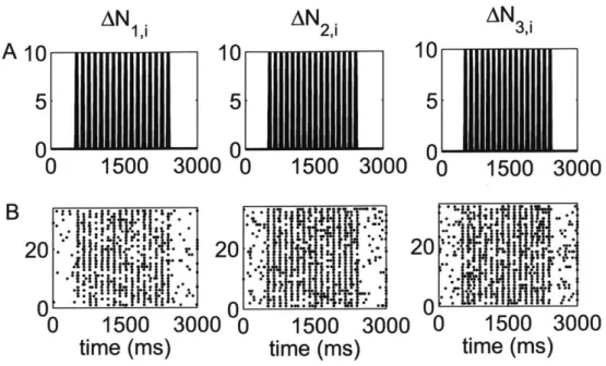
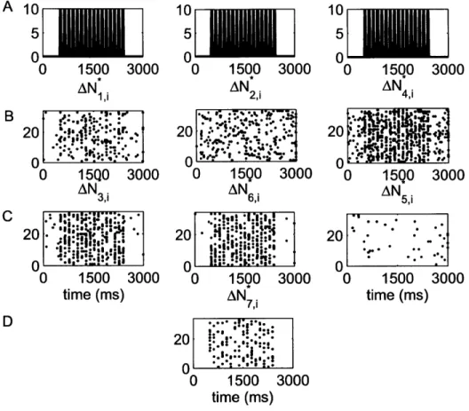
Fig.3-1 shows the standard raster plots of the simulated data. There is strong modulation of the activity of each of the neurons by the stimulus. Fig. 3-2 shows the raster plots of each of the 7 disjoint components of AN*. As the figure indicates, the parameters of the model were chosen so that the stimulus strongly modulates simultaneous occurrences from the pairs Neuron 1 and Neuron 2, Neuron 2 and Neuron 3, as well as simultaneous occurrences from the triple.

3.4 Application to goodness-of-fit assessment

Let {A*(te)

}=-

A10

10

10

5

5

5

0

1500 3000 0

1500 3000

0

1500 3000

20..

20.

20.

0

1500 3000 0

1500 3000

0

1500 3000

time (ms)

time (ms)

time (ms)

Figure 3-1. Standard raster plots of the simulated spiking activity of each neuron in a triplet in

response to a periodic whisker deflection of velocity v = 50 mm/s. (A) Stimulus: periodic whisker deflection, (B) 33 trials of simulated data. The standard raster plots show that the stimulus induces strong modulation of the neural spiking of each of the three neurons. These standard raster plots do not clearly show the effect of the stimulus on joint spiking. The effect on the stimulus on joint spiking activity is evident in the new raster plots of the disjoint events (Fig. 3-2).

in the interval [0, T). Now consider the sequence consisting of {r1m = A* (t1)} and

{jT" = A*(te) - Am E {1, --- , M - 1}. According to the multivariate time-rescaling theorem, the Trj's (f E (1, ... ,Lm}, m E (1, -... , M -1}) are mutually independent exponential random variables with mean 1. This is equivalent to saying that the random variables {u' = 1-exp(--r")} I , m E {1,- , M-1}, are mutually

independent uniform random variables on the interval (0, 1). This latter fact forms the basis of a KS test for GOF assessment much like in the case of a uni-variate point process [9].

Kolmogorov-Smirnov Test: Assume that CIFs A*(t|Ht) were obtained by fitting a

model to available data. For each m, one can use the following KS GOF test to determine whether or not the i"z's are samples from a uniform random variable on the interval (0, 1):

39

AN.3

1. Order the fi4's from smallest to largest, to obtain a sequence

{&)}mI

2. Plot the values of the cumulative distribution function of the uniform density defined as {bm = 1-12 }I against the U(m's.

If the model is correct then, for each m E {1, ... , M - 1}, the points should

lie on the 45-degree line [23]. Confidence bounds can be constructed using the distribution of the KS statistic. For large enough Lm, the 95% and 99% confidence bounds are given by bm t± 3 and bf , respectively [23].

Testing for Independence of Rescaled Times

If we further transform the um's into zm = <D-(um) (where <D(-) is the distribution function of a zero mean Gaussian random variable with unit variance), then the proposition asserts that the random variables {zf}q± are mutually independent zero mean Gaussian random variables with unit variance. That is (a) for fixed m, the elements of

{zf}m±i

{z7f}m

{zm'}

this transformation is that it allows us to check independence by computing auto-correlation functions (ACFs) (for fixed m) and cross-auto-correlation functions (CCFs) (m #i m').

A 10 10 10 5 5 0 1500 3000 0 1500 3000 0 15Q0 3000 AN AN AN 1,2 4i B . 20 M.s 1~ 20 20 .sjL $C 0 - - J All

0 15QO 3000 0 15QO 3000 0 I5QO 3000

AN 3J AN 6J AN5 C _{20 . "0} 5 0 -*3**** .,,g *AN .3I: 02 -. - . 0 1500 3000 0 1500 3000 0 1500 3000

time (ins) AN₇i time (ins)

D

20

0 0

0 1500 3000

time (ins)

Figure 3-2. New raster plots of non-simultaneous ('100', '010' and '001') and simultaneous ('110',

'011', '101' and '111') spiking events for the three simulated neurons of in Fig. 3-1. (A) Stimulus

(B) Non-simultaneous events, from left to right, '100', '010' and '001', (C) Simultaneous events from pairs of neurons, from left to right, '110,, '011' and '101', (D) Simultaneous event from the three neurons ('1'.The new raster plots of the three components show clearly the effects of the stimulus on non-simultaneous and simultaneous spiking. The AN4*,i and AN,i components of AN* show that the joint spiking activity of the pairs consisting of Neurons 1 and 2 on the one hand, and Neurons 2 and 3 on the other hand is pronounced. The AN7*, component of AN* shows that the joint spiking activity of the three neurons is also pronounced. The information in these raster plots about the joint spiking activity of neurons could not be gathered from Fig. 3-1.