Application of the extended Kalman filtering technique to ship maneuvering analysis

APPLICATION OF THE

EXTENDED KALMAN FILTERING TECHNIQUE TO SHIP MANEUVERING ANALYSIS

by

JOHN G. LUNDBLAD

SUBMITTED IN PARTIAL FULFILLMENT OF THE REQUIREMENTS FOR THE

DEGREE OF BACHELOR OF SCIENCE

and for the DEGREE OF MASTER OF

SCIENCE

IN OCEAN ENGINEERING at the

MASSACHUSETTS INSTITUTE OF TECHNOLOGY December, 1974

Signature of the Author:

D partment of Ocean Engineering December, 1974 Certified by: _ k Thet Sqprvisor Accepted by: Pr J. Harvey Ev s

D tment of Ocea Engineering

EXTENDED KALMAN FILTERING TECHNIQUE TO SHIP MANEUVERING ANALYSIS

by

JOHN G. LUNDBLAD

Submitted to the Department of Ocean Engineering in

December, 1974, in partial fulfillment of the requirements for the degree of Bachelor of Science and for the degree of Master of Science in Ocean Engineering.

ABSTRACT

This thesis dealt with the application of a particular technique in systems identification, the Kalman statistical filter, to maneuvering analyses, determining the value of the hydrodynamic coefficients to the general equations of motion. A computer program was developed for use in this identification process. _{The system that the identification was applied to} was the general class of surface vessels. The Mariner-class hull form was singled out for extensive analysis because of the availability of accepted values for the coefficients of these ships in the literature.

The identification process was conducted over a variety of experimental conditions. The results indicate a capability for the program to identify the desired coefficients with

reasonable accuracy - within five percent of the accepted true values for the individual coefficients.

It was found that the best type of maneuver was one which generates a continuously varying input of the vessel's motion paramenters, such as the sinusoidal maneuver. Addition-ally, the process was shown to be able to operate on noisy

data containing a large amount of scatter. The new coefficient estimates can be refiltered on additional passes by the process

over the same noisy data and thereby re-evaluated and updated to a new estimate. The results of this updating seems to depend upon the accuracy of the estimates obtained from the previous pass over the noisy data.

Thesis Supervisor: Martin A. Abkowitz Title: Professor of Naval Architecture

I would like to express my thanks to Prof. Martin A. Abkowitz for his supervision and encouragement over the sometimes discouraging course of this study. It is some-times necessary to have a shoulder to cry on when working with the computer.

I would also like to thank my none-too-nimble fingers for lasting until the end of this paper. I alone must take the blame for any mistakes in text and/or figures.

The financial support for the research came from the

United States Maritime Administration - project MARAD 3-36291, M.I.T. OSP 81239. Additional support came from a Sloan

Research Summer Traineeship for the summer of 1974.

All computations were done at the M.I.T. Information Processing Center (IPC),

December 18, 1974

Cambridge, Massachusetts iv

TABLE OF CONTENTS Page TITLE i ABSTRACT*o*ooooooooo(-Ooo*O*00000000*00000*000000*0000*000 ii ACKNOWLEDGEMENTO**0000000*00000*000*00oeeoeoo*ooooo*oooeo iv TABLE OF CONTENTS*ooooooooooo*eoooo*oo**ooooo*oeso*eooooe V

LIST OF ILLUSTRATIONSSO*goooo*oooooooo*oO009*0*000000000* vii

LIST OF TABLESOOOOOOO*oO*Oeo*O*oO*0*000000000000*0000000o ix

NOTATIONOO**Ooooooe**Ooooooe*eeosooooooooesooooooeoo**Ooo xi

19 INTRODUCTIONoe*oooeoooo*oe*ooo******oeogooooooooe*ooo I

II* SYSTEMS IDENTIFICATION*o*oooooeoo*ooo**Ooooo*Oo****O* 5

2ol Parametric Identificationoooooooooo*oooooooooooo 5

2.2 System Representationoooooooesoooooooo*oooosoooo 6

2-3 Identification Methodologyoooeooo*soeoooooooeooo 10

2-3-1 Iterative Procedures*e****o*oe**e*o**9**9 10 2*3*2 Statistical Filtering******9***9**99***** 11

2*4 The Kalman Filtering Techniqu.e.**.*0&#0000*00G6* 12

294*1 Derivation of the Optimum Linear Filtero. 13

2*4.2 Non-linear Extension*9**e***#*e9&**9***&* 22

III* THE ₂₅

3*1 The Mathematical Model**&*#*o*e*6G0904069*,064,, 25

3*1*1 Rigid Body Dynamics in SiX Degrees

of 26

3-1*2 The Hydrodynamic Forces and Moments*eogee 29

3-1-3 Equations of State for a Body Moving

in Three Degrees of Freedomo9***&*##*9e*9 32

3.2 Sea-Trial Maneuvers*oeoo****Ooooooooooo900000600 37

Paae

3.2.2 Zig-Zag Rudder Deflectione*e*0*006000096 39

3.2.3 Sinusoidal Rudder Def1ection*9&#@***99** 40

T

IV* APPLIGAT.LON OF THE EXTENDED KALMAN FILTER TO THE

IDENTIFICATION PROBLEM*oooooo**oo*o*Oooo**O*ooooooo&O 42

4.1 Compatibility Between the System and the Filter* 42

4.2 Noise Generation and Incorporationeeea*esooe9ote 45

4.3 The Identification Process***9*e*e9*9*e******e*e 49

Vo RESULTS OF THE IDENTIFICATION PROCESS*900*00000000000 52

5-1 A Typical Identification (Control)***o*&e**&**** 56

5*2 Variation in the Maximum Rudder Deflectionooooco 61

5*3 Variation in the Trial Lengtho*.900000960*000006 66 5.4 Variation in the Time Incrementogoe*964*06006*0* 71

5-5 Variation in the Number of Observed Primary

State Variables.ooseessooooefooooooo9o000000*00* 76

5o6 Variation in the Maneuveroo***o*o9*o*****9o99ooe 81

5o7 Variation in the Noise Leveloeeo*0006*0*60000000 91

5o8 2ed Generation Identification.oosooooooooooooooo 96

5*9 Noise Exaggerationooo*ooooo#otoeoooo***ooooooooo 101

VIo SUMMARY AND CONCLUSIONSOOOOO*000000000*00000040000000 106

APPENDIX A - PROGRAM DESCRIPTIONOGOOOOOOOSSOOOOOOO0000060 ill

APPENDIX B - THE PROGRAMoooo*ooeooooooooooooooooo*eoooooo 142

APPENDIX C - INPUT DATA DESCRIPTIONOOOOOSOOOOOOOOOOOO0000 226

HYDRODYNAMIC COEFFICIENTS000000099000*000000 230

SAMPLE DATA DECKOOOOOOOOOOOO*0900000oeeooooo 232

REFERENCES*0006000000000000000******Oooooooooooo*ooo000*0 234

LIST OF ILLUSTRATIONS

Figure No.

2-1 Block Diagram of Optimum Linear Filter*...

3-1 Rectangular Coordinate System... 4-1 Imprecision in Noise Definition... 5-1a Filtered States - Typical Identification...

5-1b Coefficients - Typical Identification...

5-2a Filtered States - Variation in Maximum Rudder

Deflection...

5-2b Coefficients - Variation in Maximum Rudder

Deflection...e..e...*.e.*eee*e.eeoeeeo 5-3a Filtered States - Variation in Trial Length....

5-3b Coefficients - Variation in Trial Length...

5-4a Filtered States - Variation in Time Increment..

5-4b Coefficients - Variation in Time Increment.,...

5-5a Filtered States - Variation in the Number of

Measured Primary State Variables...

5-5b Coefficients - Variation in the Number of

Measured Primary State Variables...

5-6a Filtered States - Variation in Maneuver

(Zig-zag Step Rudder Deflection)...

5-6b Coefficients - Variation in Maneuver

(Zig-zag Step Rudder Deflection)...

5-6c Filtered States - Variation in Maneuver

(Single-Step Rudder Deflection)...

5-6d Coefficients - Variation in Maneuver

(Single-Step Rudder Deflection)...

5-7a Filtered States - Variation in Noise Level...

5-7b Coefficients - Variation in Noise Level...

vii Page 21 27 48 58 59 63 64 68 69 73 74 78 79 84 85 88 89 93 94

Figure No.

5-8a Filtered States - Second-Generation

Identilfication...

5-8b Coefficients - Second-Generation Identification

5-9a Filtered States - Variation in Noise

Exaggeration...

5-9b Coefficients - Variation in Noise Exaggeration.

viii Page 98 99 104 105

LIST OF TABLES

Table No.

4-1 Summary of the Computation Steps... 5-1a Conditions for the Typical Identification... 5-1b Coefficient Identification for the Typical

Case...0*...o

5-2a Conditions for the Variation in Rudder

Deflectio..Ooo@0000. 00.00 0000o000e00e0e

5-2b Coefficient Identification for the Variation

in Maximum Rudder Deflection...

5-3a Conditions for the Variation in Trial Length..

5-3b Coefficient Identification for the Variation

in Trial Length...o...o...

5-4a Conditions for the Variation in Time

Incremento.. ₀ ....o ... o.... .eo 00.000000000 5-4b Coefficient Identification for the Variation

in Time Increment... 00 5-5a Conditions for the Variation in the Number

of Measured Primary State Variables00. ...0

5-5b Coefficient Identification for the Variation

of the Number of Measured Primary State

Variables...

5-6a Conditions for the Variation in Maneuver

(Zig-zag Step Rudder Deflection)...

5-6b Coefficient Identification for the Variation

in Maneuver

(Zig-zag Step Rudder Deflection)...

5-6c Conditions for the Variation in Maneuver

(Single-Step Rudder Deflection)...

5-6d Coefficient Identification for the Variation

in Maneuver

(Single-Step Rudder Deflection)...

ix Page 51 57 60 62 65 67 70 72 75 77 80 83 86

87

Table No.

5-7a Conditions for the Variation in Noise Level...

5-?b Coefficient Identification for the Variation in Noise Level...* ...

5-8a

Identification...*.*...*....

5-8b Coefficient Identification for the Second-Genration Identification...

5-9a Conditions for the Variation in Noise

Exaggeration...*...

5-9b Coefficient Identification for the Variation

in Noise Exaggeration...*....*...*...

x

95

97

NOTATION

Lower case letters represent scalar quantities: x

Lower case leters, underlined, represent vectors: x

T

Vector dot product: XTx

Upper case letters represent matrices: E

The superscript T represents the matrix transpose: ET

A bar over either a scalar or vector represents the mean value of that quantity:x

INTRODUCTION

The naval architect must be able to predict the various motions of an ocean vehicle in order to design a vessel which can meet the required aspects of operability under which the ship will function. Without this knowledge, little can be said of the ship's capabilities with any certainty until the system is actually built. An accurate model of the vessel is thus of primary importance for design purposes.

The dynamics of an ocean vehicle can be described theor-etically in terms of a general set of motion equations. The utility of this set of equations which can accurately predict the motions of a ship should be readily apparent.

The equations of motion are derived in a number of ways throughout the literature.. That method which implements the vector calculus is presented later in this work. The equations' structures are such that they may be applied to many diverse systems, with the judicious choice of coefficients to the equations setting their structure to the particular system at hand. The specification of these coefficients sets the model to the system and is the problem area toward which this work is oriented.

Unfortunately, the exact numerical values of these

hydrodynamic coefficients are difficult to attain. Hydrostatic 1

2

and hydrodynamic theory permits specification of only a few of the parameters. Through potential theory, the acceler-ation derivatives can be calculated with reasonable accuracy,

though they are of minor importance in terms of the general equations.

The coefficients associated with the criteria for dynamical stability in straight line motion,

Yv(Nr-MXGu)-Nv (Yr-mu)> 0,

namely the velocity derivatives, are unattainable to

sufficient accuracy for displacement hulls through present theory. For these and many other cases, one presently must resort to captive model tests in the towing tank. The

consequence of this is the Introduction of scaling effects inherent in the modeling of ship systems to the correct

Froude number and, by necessity, the neglecting of Reynold's number.

There are two principle means of running model tests at present. One uses the rotating-.arm mechanism. The other more popular method incorporates the planar motion mechanism. For both methods, the forces and moments exerted on the

model hull forms are measured by dynamometers as the model is put through various constrained maneuvers. These forces and moments are then plotted as a function of the motion variables. The slope.through the equilibrium condition,

usually the origin, of this function then gives the relevant force or moment derivative. Quite obviously, this is not as accurate a procedure as one would desire because of scale effects and the difficulty of attaining certain of the non-linear coefficients.

A possible alternative to this traditional approach is

derived from modern control theory. Systems identification consists of a set of theories and their applications,

capable of assigning the most suitable numerical values to the variables and coefficients of the equations describing the state of the system. These equations of state consist of the motion equations as well as functions representing the measured motion responses, both assigned levels of uncertainty in their structure and recording capabilities.

One of the methods used in systems identification is statitical filtering. By taking advantage of the estimated uncertainties, or noise, as well as recorded trajectories of the ship motions, the statistical filter is capable of choosing values for these coefficients which minimize the error between the recorded and calculated state values. The specific technique of filtering used in this work is the Kalman filter, an optimum linear filter which was extended to handle non-linear systems.

The main body of this thesis consists of two parts. In Chapters II and III, the theory and equations describing both the system and the identification technique are given.

4

The equations of motion describing the state of the system are developed, as well as an optimum linear filter and it's non-linear extention for use in the identification.

The second part of this thesis, contained in Chapters IV,V and VI, applies the theory to a practical problem -the identification of -the hydrodynamic coefficients of a Mariner-class surface ship. This type of vessel was chosen primarily for consistency with previous studies in the area. Additionally, the coefficients for this class vessel are well documented in the literature and permit a realistic appraisal of the identification results given in Chapter V. Conclusions and future considerations are stated in Chapter VI.

A listing of the general program developed for this study, as well as a description of its usage, are given in the Appendix. Also included are various and sundry items

useful in this work and hopefully for any continuation of these studies.

SYSTEMS IDENTIFICATION

2.1 Parametric Identification

Inherent in the understanding of any dynamic system is the ability to model that system accurately through a series of differential equations. The general identification and specification of any system requires that the general

structure of the system as given by this mathematical model be known, although the particular values of the parameters in the model need not be specified. For a system in this form, classical identification techniques can be employed determining the particular parametric values. This is referred to as parametric identification. The mathematical equations usually involve what are termed the state variables of the system and their derivatives, along with various

constant coefficients to these variables. The coefficients set the model for the particular system or conditions under consideration. It is the values of these coefficients which need to be determined.

In ocean vehicle dynamics, the coefficients primarily relate to the hydrodynamic forces and moments exerted upon the body in response to arbitrary disturbances from

6

equilibrium. These coefficients, which take the form of first, second and higher order force and moment derivatives, may be either completely unknown or reasonably estimated to within a degree of uncertainty. Part of the uncertainty arises from the methods involved in their estimation - model tests and full scale trials. Precise response trajectories of the vehicle motions are difficult to attain. Typically, for systems of this sort the deterministic, or precise, model is waivered for a simpler indeterminate model, where minor higher order terms as well as indeterminate noisy additions to the responses are incorporated into a single noise variable. This concept will be further developed later in this work.

2.2 System Representation

The systems analyst works is a realm defined by state variables and state-space representations of dynamic systems.

A set of state variables are simply those variables which,

along with a set of initial conditions, can be used to completely describe the dynamic state of a system - past, present and future. For a static system, this definition is trivial. However, since one usually deals with dynamic systems whose state is ever changing with time, the ability to so model that system is crucial to it's identification.

literature. Its usage is somewhat arbitrary, though

frequently it refers to the set of velocity parameters. 8

)

ident-ification procedure - the measured parameters of the vehicle motions. These may include orientation as will as motion variables.

The state-space representation of the dynamic system is that set of equations incorporating the state variables which forms the model of the system.

x = f( x,u,t)

z = h(x,u,t)

x(t0)X

Here the state variables, x, and the input variables, u,

are used in the motion function, f, giving the time rate of change of the state variable and the measurement function, h, giving the measured output, z.

Frequently, the actual structure of the system is known, except for a set of parameters or coefficients, 2.

See Notation - the bar under a lower case letter indicates a vector quantity.

8

As stated earlier, this structure can be simplified by neglecting extraneous higher order terms. A modification to the equation structure involving a single uncertainty term, w, compensates for this adjustment. Similarly, any uncertainty in the measurement function can be included in another uncertainty term, v. The state-space representation then takes the somewhat more complex though useful form,

X = f(x,u,p,w,t)

z = h(x,u,p,v,t)

x(t0) = X

A significant simplification in both the structure of

the above representation and eventually in the computation incorporating the model can be made through the following assumptions about the system under consideration:(16)

(i) The mathematical model and the measurement function are time invariant.

(ii) The system structural uncertainty and measurement noise are linear, and add directly to the equation of state.

(iii) The output measurements are linear functions of the state of the system, and are

(iv) The model coefficients are constants of the system while under observation and hence are the objective of the identification.

The first assumption is the most crucial since the loss of the assumption implies that any identification on the system is valid only over the period of observation and thus cannot be extended to the general case. The time invariant assumption, however, can be lifted if the relationship between the structure and time is known. For a quasi-static structure which is only slowly time-varying, the time invariant

assumption can be made, though with some caution.

The dynamic state-space representation under these as assumptions is thereby reduced to,

0

x=f(x9uP) + w (2.1)

z = Hx + v (2.2)

For cases such as in this study, where the measured output is assumed to be in direct correspondence with the state of the system, the measurement function is simply the identity matrix.

10

2.3 Identification Methodology

Many different techniques exist for applying the system representation, eqs. (2.1) and (2.2), to the parametric

identification problem. The literature abounds with procedures, many primarily oriented toward specific identification

problems.(7),(10),(15) The trick then becomes the matching

of the more adept procedure to the situation at hand.

2.3.1 Iterative Procedures

One of the more general methods applied to ship maneuvering, investigated by Brinati, was the model reference technique, an iterative process. This procedure

is one of the more conceptually simple identification techniques in current use. It can best be described as a brute force interpolation. The mathematical model is set except for one or two of the coefficients which are varied uniformly in an attempt to find those values which minimize

the error function between the model and the actual data. This method was shown to work well. However, the limitations under which it must operate - limited noise levels and a minimal number of observable coefficients per trial, seem to limit its utility in extensive design applications.

2.3.2 Statistical Filtering

An alternative approach and one which has received a great deal of attention in the past decade is that of

statistical filtering. Part of this popularity and utility comes from the fact that it provides an optimum use of all available information about the system. This includes

statistical estimates of both the noise in the system and its state.

Much of the initial theoretical work on statistical estimation and filtering was performed by Weiner,(1,) in the 1930's. It's applicability to systems analysis was developed by Kalman (11),(12) in the 1960's. He showed that an optimum

linear filter, based on the covariance matrix of the state estimation errors can lead to a minimum error in the final estimate of the state of the system.

There are two major disadvantages to the Kalman filtering technique, neither of which had a very serious effect upon this study.

(i) The filter has a linear derivation and there-fore is valid only for linear systems.

(ii) It requires a reasonable, but not necessarily accurate, estimate of the system and noise parameters before their identification may proceed.

12

For ocean vehicle systems, the second problem is incon-sequential. Reasonable estimates can be made from vehicle coefficients which are presently in the literature, or have been attained from model tests of the class of vehicle desired by traditional methods. For other types of systems, where this estimation problem might become significant, on-line identification techniques are being developed which can work in conjunction with the Kalman filter, but which initially need no precise estimate of the state or noise characteristics.

The restriction to linear systems is also of little

concern for those cases where ship maneuvering can be limited to small linear disturbances. This permits the use of

simplified linear models available in the literature.(6)

For the general case, however, the restriction of linear modeling is not acceptable. The methods used by Brock(4)

and described here lift that restriction and permit the extension of the Kalman filter to the non-linear case - a development which may not be theoretically strong but which works quite well all the same.

2.4 The Kalman Filterinw Technique

The Kalman filter was the identification technique used in this work. It is a statistical filter for use in the presence of uncorrelated white noise. Through use of the Kalman filter, the identification problem is reduced to a

state estimation of the dynamic system. The filter development follows for a linear system which in turn is followed by it's logical extension to the non-linear case.

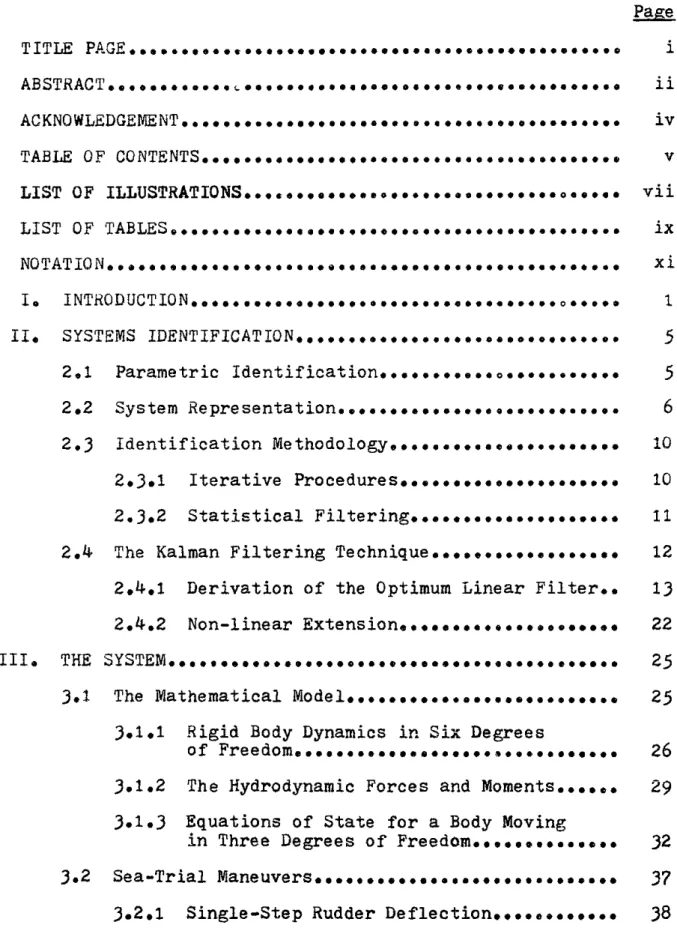
2.4.1 Derivation of the Optimum Linear Filter

Earlier in this chapter, the equations for the

state-space representation of a dynamic system, eqs. (2.1) and (2.2), were developed,

x f(x,u,2) + w

z = Hx + v

where a linear relationship between state and output has been assumed. For simplification in that which follows, the noise factors, w and v, will be discarded for the time being. The dynamic system representation is therefore reduced to,

x = (x,u,p) (2.3)

z = Hx (2.4)

Given a system defined by these state and measured out-put functions, one desires to estimate the true state of the system at some time t. If numerous measurements of the system

14

are taken, a realistic assumption for most physical systems is that the values attained will approximate a Gaussian distribution0 Therefore, the best estimate of the state of

the system , will be that which approaches the mean, L, of the system,

X = x xP(xjz)dx

000

Any error in this estimate can be defined by

e = x - x

and the covariance matrix of these errors by

E = (*-x)(k-x)T

-T

e e (2.5)

One of the characteristics of a Gaussian or normal distribution is the fact that the mean of x specifies the maximum of its probability density function (PDF),

P(i) = max

[P(x3

Therefore, a proper method for determining the optimal estimate of x is one which would determine that x which

maximizes it's PDF. The standard form of the Gaussian PDF for a random variable, y, is given by

P(y) = e 20OD<Yo5 0)

This can be extended to describe a system of n state variables as

S(X-)U'xx)T/ ₂E

P(x) (= n n/2 .1/2e

=(2n9)" E~t

where E is the variance, defined as the square of the standard deviation, a2. The problem is then one of maximizing P(x), under the constraint imposed by the measured output

z = Hx

Since log [P(x) attains a maximum for the same value of x as P(x), the problem can be rewritten, using Lagrangian multipliers, as the maximization of F(x), where

F(x) = log P(x) + XT (z-Hx)

= log - i'-x)x x)T/2E + XT (z-Hx)

16

The variation of F(x) with x is given by

dF (x) -T d(x-x)TE~I dx

-x

aT

Taking the transpose of both sides yields

(-x) (Ei)T =

x

-x)=

ET

K =

i-X

From the measurement function,

z = Hx

= H(0 - X EHT)

or,

= (Jj5- z)/HEHT (2.7)

Substitution of eq. (2.7) into eq. (2.6) gives

x =QX"+ [(z-)/HEHT] EHT

=x H + EHTHEHTJ -(Z- (2.8)

This then is that value of x which maximizes the PDF for the function and, by definition, is the optimum estimate of the state of the system at time t.

It can be shown that if one includes the measurement noise, y, in the eq.(2.4), having its specified character,

then the more general form of the state estimate is

Ix

where,

18

In order to determine the new covariance matrix for this optimal estimate, x , one need only substractx from eq.(2.9), arriving at a value for e. From the relation

E =e eT

one arrives at the updated matrix

E= E - EHT T + R) HE (2.11)

Eqsa(2.9) and (2.11) can be somewhat simplified and possibly more easily understood by defining the new variable K, the gain.

K = EHT (HEHT + R)MI (2.12)

Then, eqs.(2.9) and (2.11) reduce to

'% = +K(z-Hx) (2.13)

(2.14)

E' = E - KHE

At this point, the process noise in the state equation can be re-introduced into eq.(2.3) as given in eq.(2.1).

0

The optimum estimate for x will then take the form

x = f(x,u,2) (2.15)

since the process noise is defined as being of zero-mean. This equation can be rewritten as

x = Bx (2.16)

where B is a matrix of coefficients acting upon the state variables.

B = ---- (2.17)

The error in the state estimate is seen to be

A9 4

e =x-x

=Bx- (Bx +w)

The time derivative of the error covariance matrix, E, is then written as d T E = .--- (e e dt -* T * =e e + e e

20

or finally,

E=BE + EBT + (w w)

The process noise covariance matrix, Q, is defined as

Q = w w (2.18)

The time rate of change of the error covariance matrix can therefore be converted to the form

*T

E = BE + EBT +Q (2.19)

This then is the controlling equation in the variation of the covariance matrix in conjunction with the measurement function over time.

The estimation problem can thus be completely described

by eqs. (2.13),(2.14),(2.15) and (2.19). When a measurement

of the system is taken, eq. (2.13) determines the optimal

As

estimate,, x', of the state variables at that time. This it does by maximizing the system's PDF based on the previous

estimate of the system,

12,

eq. (2.14) as a function of the matrix calculated for the previous measurement. Eqs. (2.15) and (2.19) are integrated to update the state and error covariance matrices before the

next measurement. These new values of the state and co-variance matrices before the next measurement. These new values of the state and covariance matrices are then used to again optimize the system's estimates and the process repeats itself.

r

~

- M

I

rn

M-.

ON

Phys ical j~easurement,

Systemv

+ f IOH

I- I II

L om dm NJdmII IP

goal--- ' M

Optimum Linear Filter

Simulation i

1i+

I>

EHI

1 mo8w- m. M do

Block Diagram of Optimum Linear Filter Fig. 2-1.

22

2.4.2 Non-linear Extension

The derivation of the equations relating to the statistical Kalman filter was done for a linear system,

0

x= f(x,u,P,w)

z = h(x,u,2,v)

and indeed, can be applied only to those systems whose dynamics can be considered linear functions of x, u, p and v or w. However, it is possible to extend these equations to the cases where the dynamics of the system must be

described by non-linear functions. This linearization of non-linear equations gives one the versatility of applying the filtering technique to a wider class of physical systems.

Assuming eqs. (2.1) and (2.2) are continuous and differ-entiable over the region of interest, the state variables can be written as

x = x +6x

z = z +bz

-o

about the initial values,

6x = --- 6x +

-- x - w

-bz = ---o6x + -- o by + 00

The values of x and z can be assumed to be close to the initial values so that 6; and bz can be considered linear functions of 6x This assumes that 6w and 6v are equal to w and v respectively, which follows from their being uncorrelated.

The linear derivation described earlier can then be used to get the optimum estimate of 6x. The equations for the non-linear filter are thus of the same form as those developed for the linear case, with minor redefinitions of the matrices involved.

x = f (',u,e) (2020)

x = X1 + ESHT (HEOHT + Rn)al

(z-x)

n-

-E = BE + EBT + Qn (2.22)

E = E' - E'HT (HEOHT + Rn)

F

where,

24 H = T n= - -Q = -- --n IN B

For the assumptions under which eqs. (2.1) and (2.2) were developed, namely additive linear noise and a linear measure-ment function, the noise covariance matrices, Rn and Qn,

THE SYSTEM

The system under consideration in this work is a Mariner-class vessel operating in unrestricted waters. Under equil-ibrium conditions, it is assumed to be moving at a constant forward speed. We are interested in determining the effect that various deviations from the equilibrium condition will have upon the motions of the ship. To do so requires a

model which accurately portrays the vessel under any and all conditions in which it may be found.

3.1 The Mathematical Model

The best method of simulating a dynamic system is to mathematically recreate it through a series of differential equations which can accurately describe its motions. The mathematical model used in this work, developed by Abkowitz, considers the vessel as a rigid body of constant mass with a stationary center of gravity. Alternative models have been developed in the literature for similar systems, as well as, those special cases not included in this model.(8)

A body moving in a fluid medium is considered to be a acted upon by a system of fortces and moments. These can be

26

resolved by considering two sets of forces and moments, each of which is equivalent to the other at equilibrium. First, one can consider the body's rigid structure and the forces and moments due to it's mass and the motions of that mass -velocities, accelerations, moments of inertia, et cetera, independent of the body's shape. Secondly, one can consider the forces and moments arising from the medium itself,

termed the hydrodynamic forces and moments. These act upon and are initiated by the body's shape - the dynamics of its interaction with the fluid medium. The subsequent motions of the body in the fluid through dynamic equilibrium arise from equating the two systems of forces.

3.1.1 Rigid Body Dynamics in Six Degrees of Freedom

The dynamics of the origonal body structure are ultimately derived from an understanding of Newtonian mechanics.

F =

A

- dt

dt

M = (Angular Momentum) = KT + MT + Nt

- dt

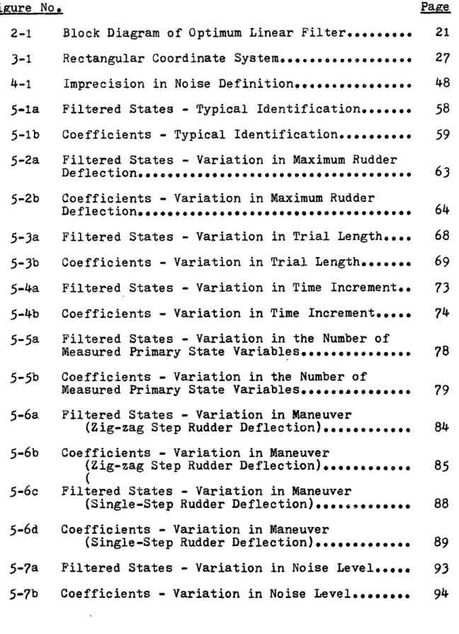
One can consider a rectangular coordinate system with arbitrary origin not necessarily at the center of gravity of the system, but parallel to the principle axes of inertia through the center of gravity. The system can thus be shown

in the form of fig. (3-i), CG M N Y

z

Fig. 3-i, Rectangular Coordinate System

where the relevant forces and moments are as indicated. RG is the vector displacement of the origin from the center of gravity.

Using this notation, the force equation becomes,

d

F=my- (U + QxG

under the constant mass assumption, where

= pt + qj + it

R

WL ip

28

and is defined as the angular velocity of the center of gravity about the chosen origin. Expansion of the equation yields the force components along the principle axes.

x -2+2

X = TLu + qw -rv -xG (q +r )

+ G(pq-r) + zG(pr+q)J (3.1)

Y = m v + ru - pw - YG(r+p) + zG(qr-p) + xG(qp+r) (3.2)

z =M w + pv-qu-zG(p 2+q 2) + xG(rp-q) + yG(rq+p) (3.3)

In a similar manner, the moment equation can be shown to be equivalent to

whereG+OG

where

dt x

The moment components about the principle axes are then given

by the equations

K = I + (Iztl y)qr + mYG( + pvequ) -zG(v +ru - pw)

+X G Ypr-4 )soxGzGpq 4 _{) + yGZG(r}

= yq + (I'-Iz)rp + m IzG( + qw - rv) - xG(w + pv - qu)

1** _{( 2 r}

( ,5

+ yGzG(qP-r) - yGG(qr+p) + xGGa -rJ

N = Izr + (IY-I )pq +, mlxG(v + ru -pw) - yG(u + qw-rv)

" Z 0(rq-p) - Z yprprqiq G Gp)J(,6

+ G G GYG r+q) + yG G 22)(I6

The rigid body structure of the dynamic model can there-fore be summarized by eqs. (3.1) through (3.6) for a vessel of constant mass and arbitrary origin of its coordinate system.

3.1.2 The Hydrodynamic Forces and Moments

The dynamic forces and moments acting upon the body in a fluid are functions of the body itself, its motions and the medium through which it passes. For a given body oper-ating in a particular fluid, these functions are dependent only upon the body's movement.

F

= g(R

2,

For this work, it is assumed that the body is operating in unrestricted waters, therefore negating any effect of the

30

orientation parameter, R , on the dynamics. The only effector force and moment contributions will come from the rudder

deflection, 6, neglecting higher order terms such as 6 and 6.

F. .

g(UJU,

2,,6)

M Is

The function in eq. (3.7) can be expanded through a Taylor series expansion, assuming the function is continuous and

analytic over the region of interest. This assumption is valid under normal operating conditions.

The multi-dimensional expansion is done about a nominal condition, in this case the equilibrium condition of constant forward motion, in terms of the individual components of the functional quantities. Looking at the force equation,

F = F(u, v, w, p, q, r, u, v, w, p, q, r, 6)

the expansion becomes a lengthy equation of the form

F + ( ) ( A u ) + *** +A ( ) ( Au 0)2

2

+ 0+ ()u> O( _{Au )( AV)} +00

+)

L u terms

It will be seen that many of the terms in eq. (3.8) can be eliminated by employing the proper assumptions.

Two simplifications are now in order. First, standard shorthand notation will be used throught for the force and moment derivatives, =F 3x o -x. Secondly, (x d o x~i( o

Under the equilibrium conditions of straight ahead motion at constant speed,

(xi 0 = 0

and

(xi) ₌

xi

for all xi except u, which doesahave a non-zero equilibrium value. _{Therefore, the hydrodynamic forces and moments can} be portrayed as

32

FA + (A) + ** +

i[Fu(

- o -U 21 -uu -UV

+.. + [F ( Au)3 + * + higher order

+ [7UUUJ terms (3.9)

3.1.3 Equations of State for a Body Moving in Three Degrees of Freedom

The rigid body structure of the dynamic model for a body of constant mass and arbitrary center of gravity, moving in six degrees of freedom was given in eqs. (3.1) through (3.6). Similarly, the hydrodynamic forces and moments acting upon

a body with six degrees of freedom are derived in the form of eq. (3.9) from the Taylor series expansion. With the system under dynamic equilibrium, the hydrodynamic forces and moments are solely responsible for the forces and moments acting on the rigid body, and hence the motions of the body through the fluid. Therefore, the two systems of equations can be equated to determine the resultant motions in six degrees of freedom.

Hydrodynamic and

)

hydrostatic forces reaction (3.10)

and moments

)

This general case does not always apply to every system, however. _{For this study, the body was constrained to only} three degrees of freedom - a surface ship operating solely within the horizontal plane. Additionally, it was assumed

that these horizontal maneuvers do not excite rolling motions. This assumption applied to the Mariner-class hull form is

adequately valid under normal operating conditions. It will also be assumed that yG is located along the longitudinal plane of symmetry.

Under these conditions,

yG= = w = p = q = w = p q = Z = K = M = 0

for any time t. The equations used in eq. (3.10) can therefore be reduced from the general case to that for only three degrees of freedom, with substantial simplification in structure.

The rigid body forces and moments in the horizontal plane, excluding roll, are

X = m Cu- rv - xGr *(3.11)

Y = m (v + ru + xGr) (3.12)

N = Ir+ MXG(; + ru) (3.13)

while the hydrodynamic forces and moments for the same case are given by the Taylor series expansion of

= 0 ,

Y = Y(u, v, r, u, v r,

6)

N = N(u, v, r, U9 V9 r, &) (3.16)

Brinati showed that numerous additional terms in the expansion of the hydrodynamic structure could be dropped by additional assumptions. These included cross-coupling

between the acceleration and velocity terms, negligible second and higher order terms, and negligible contributions from symmetry considerations. Applying these assumptions, which are quite valid, one arrives at the following form for the hydrodynamic structure.

XX+XAu+V+1-X(u2 2 2

X = X, + X( _{o u} AU) + X 0u + _u 2 _Luu uu A u)2 + X v

_V

+ X62 + Xrvr + Xr6b + Xv6 + Xuuu )3

+ Xvvu"2( A u) + Xr2 ( Au) + X 62( A u)

+ Xvruvr( Au) + XV₆ uvb( A u) + X ₆rb( A u) (3.17)

Y = Y + YvV + Y6 + Yvuv( Au) + Yrr + Yrur( Au) + Y6u6( Au)

o v 3 +Y r

vu 6r 1 ru

+ Lvv 3++Yrrr +6663 + 2[vrrv

+ YV_{6 6}v62 + Yvuuv( Au)2 +y rv 2 + Yr66 r2

+ Yruur( Au) 2 + Y6vv6V2 + Y6rr r2 + YOuUN6(Au)21 + Yvr6vr6 (3.18) N=N₀ + N v + N r +Nb 6 + N v( au) + N r( Au) + N₆ 6( Au) + ' [Nvvvv3 + Nrrrr3 + N_{6 6}63 1 + N yr2 +Nvb 2 +N v(Au)2 2 + vrr v66 vuu + Nrvvrv + Nr6 2 + Nruur( Au)2 +Nb6vvv2 + N b6rr + N6uu6( Au)2

]

A further simplification can be made in eqs. (3.17), (3.18) and (3.19), by dropping those terms which individually have negligible effect upon the eventual motions of the ship, without unduly altering the model. This reasoning is some-what similar to the dropping of the fourth and higher order terms from the expansion. For all cases, dropped terms, if small enough, are in actuality compensated for in the indeter-minate model by the uncertainty term. Possibly the most

important reason for this simplification is not so much in reducing the equation structure, but rather in what will be. shown to be a detrimental effect by these minor terms on the identification process itself. Brinati conducted an

exam-36

ination of these equations and was able to separate a number of minor terms. The results of his work were not verified for this study because of time constraints, but were used in the equation development.

Equating the resulting hydrodynamic structure with that developed for a rigid body under constraint of maneuvering

in the horizontal plane, and solving for the acceleration terms, leads to the following set of state equations.

u = f1Cm - XQ) (3,20) (Iz ₂ Nf₂ m G r 3 (3.21) f4 (m -Y*)f3 _{0- (mxG} - N*)f2 r = (3.22) 4 where,

f X +X(AU)+1 x AU)2+l X (Au)3 1 2

1 o u + uu uuu 2 Xv +( X x )r 2 + x 6 2 + (X +m)vr+ X ₆ 1 1 2 2 o v r 66 666 Yrvv 1 2 + 1 Y 6 v2

1 3+ 1 2

f = N0 + Nvv + (Nr -mxGu)r + N66 + 1 N6666 ++ Nrvv

1N 2

2 6vV

4 = (m - YQIZ - NP) - (mxG - N)(mxG - Ye)

Eqs. (3.19), (3.20) and (3.21) then, describe the motions of the vessel in the horizontal plane with three degrees of freedom, Together, they form a set of state variables which, along with the initial conditions of the problem, completely describe the past, present and future motions for any given input. This dynamic model is complete, except for these initial conditions, and forms a sufficient set of equations for the work of this study.

3.2 Sea-Trial Maneuvers

Of primary importance in any maneuvering trial is the

proper planning for that trial. Especially in the type of identification process proposed here, it is necessary to know what effect different maneuvers will have on the ability to identify the different hydrodynamic coefficients. It is desirable to know what measurements to make, which motions

to record under the various conditions of gradual accelerations, sudden changes in velocity, steady state velocities or the

38

For these reasons, several different maneuvers were used in this study and are described here. As stated earlier, the only control surface considered in this work was the rudder and it's deflections. This was incorporated into the general equations as the variable 6.

3.2.1 Single-step Rudder Deflection

Formally, the single-step rudder deflection can be de described as a step function of the form

6(t) = 6,9 6(t) 6 I t<0 t>o 0 t

Graphically, this corresponds to the case where the vessel goes into a constant turn in the steady state.

t _'

R2>-Previous to the rudder deflection, all velocities and accelerations are zero except u. However, u is an unmea-surable motion by conventional methods and for the most part

will be neglected. As the effect of the rudder deflection is felt by the vessel, all velocity and acceleration terms become non-zero until the ship reaches it's steady state

turning radius. At this point the acceleration terms v and r have non-zero values for the remainder of the trial. For large rudder deflections, a distinct speed reduction occurs due to the tight turn.(2)

3.2.2 Zig-zag Rudder Deflection

Again, this maneuver can also be formally described by the step function,

0, t<0, t 200 6(t) = 3, ot<100 -6, 100<t<200 6(t) +6 0 100 _{200 t} -b

This definition is perhaps not completely realistic to real-life situations at sea since no time-lag is incorporated into

it's structure. However, for the purposes of this study, it is an acceptable representation. Pictorially, I A to PIL

the vessel is seen to go into one steady turn followed by the opposite steady turn and finally achieving the new equilibrium state of constant forward speed, though not necessarily at the original orientation. Essentially there are three steady state conditions during the maneuver. The situation for the motion parameters in the steady state turns is identical to that discussed for the step deflection. For the straight ahead motion at constant speed, both the velocity and acceleration terms are reduced to zero.

3.2.3 Sinusoidal Rudder Deflections

This deflection is simply a sinusoidal motion of the rudder with a maximum displacement corresponding to 6 and with the specified period, T.

6(t) = 6 sin at

6(t)

+6

-6

-T

-The motions of the ship will follow the rudder deflection in a sinusoidal manner, with a slight time lag.

t~~~~ ~ 0-0 01-ft-% b- 0

The important point for this maneuver is that the velocity and the acceleration terms are in a constant state of flux. At no point during the trial, after t, is the steady state

condition established for any of the motion parameters. This gives the identification process a continually changing system upon which to operate.

Chapter IV

APPLICATION OF THE EXTENDED KALMAN FILTER TO THE IDENTIFICATION PROBLEM

4.1 Compatibility Between the System and the Filter

In Chapter II, the concept of parametric identification was developed as a means of system identification applicable to those dynamic systems whose general structure was known, but whose specific parameters or coefficients were unknown. The structure of the indeterminate model was given as

x = f(x,1u,2p) + w (4.1)

z = Hx + v (4.2)

where the imprecision of the model is represented by the uncertainty terms, w and v.

The utility of statistical filtering as a method for

solving the identification problem was shown and the equations for the optimum linear filter, as developed by Kalman, were given. _{These equations were extended to the non-linear form.}

x = f(, uIt )(4.3)

x + EkF (HESHT + R )-1(z - Hx) (4.4)

Tn

E=BE + EBT + Qn (4.5)

E = El - E'HT (HE'HT + Rn F 1 _{HE (4.6)}

The general model for an ocean vehicle was developed in Chapter III for a surface ship moving in the horizontal plane without roll. f /(m - V)(4.?a) u 1 u (I -N)f2 - (MxG f3 (4*7b) 4 (m-Y.)f3 - (mxG - N,9f2 (4.7c) 4

-where f , f2pf3 and f4 are as before. This gives the general structure of the system (a vehicle under maneuvering) and

identifies that system except for the hydrodynamic coefficients. The initial conditions which specify the dynamic condition of the system are those for which the equations were developed, namely straight ahead motion under constant speed.

By combining these steps, the ability to use the extended Kalman filter to identify the hydrodynamic coefficients of

44

the equations of motion can be attained. First, however, some minor changes must be made in the above development.

The state vector must be extended to the augmented state,

x = (x₁, x₂, n 9tl' 2* '

by the inclusion of the unknown coefficients. In this manner

the Kalman filtering technique which identifies, or more correctly estimates, the state of the system can be used to identify the coefficients under observation by including them in the state vector.

The input function of the ocean vehicle is known and is frequently a function of time. This removes the time in-variant assumption in the structure of f. However, since the function of time, u(t), is known, it can be incorporated into the model and as stated earlier, is an acceptable alteration.

These two redefinitions reduce eq. (4.1) to

x = f(x,t) + w = B(t)x + w (4.8)

which is compatible to that used in the definition of the extended Kalman filter.

Finally, from the assumption of linear additive noise contributions to the equations of state and measurement

function, the process and measurement noise covariance matrices,

R=R n

From these alterations, the system, a Mariner-class surface vessel in maneuvering, and the identification tech-nique, statislical filtering, may be applied to the problem at hand. This does not necessarily-imply that statistical filtering in particular or system identification in general can lead to the complete specification of the system

structure. It does mean, however, that one is now in a

position to apply the system to the technique and see wether or not an identification capability does indeed exist.

4.2 Noise Generation and Incorporation

Up to this point, very little has been said concerning

the noise contributions, w and v, to the system structure and measurement function. In Chapter II, one of the dis-advantages of the Kalman filter was stated to be that the statistical characteristics of the uncertainty terms had to be specified. This is true, though the estimation of these characteristics for many cases is relatively straightforward.

The process noise, w, expresses the uncertainty in the structure of the mathematical model. This arises from the truncation of the Taylor series expansion for the

hydro-46

dynamic structure of all terms over third order. It may also incorporate any unknown contributions from the input function, i(t), or any spurious deviations from the assumptions used

in developing the equations of state. Excitations from the enviornment are also included in the process noise.

The output uncertainly is expressed as a measurement noise, v. As for the process noise, this term includes all

unknown structural aspects of the measurement function, H. For this study, since the measured output is assumed to directly correspond to the actual state of the system, any

deviations from this linear correspondence are represented by v.

The noise contributions are both treated in a similar manner and are felt to be similar, statistically. Both are assumed to be stochastic processes, with uncorrelated, zero-mean, Gaussian white noise. The Gaussian probability density

function (PDF) for the uncertainty values is a reasonable assumption for most physical systems. From the central limit

theorem of general probability theory, it can be shown that the sum of a large number of independent effects has a

Gaussian distribution, regardless of the statistical properties of the small effects individually. The uncertainty terms can

therefore be considered Gaussian in nature and treated as random variables for simple incorporation into the model structure.

w = E [w ] = 0

v = E[v] = 0

Q = E[wwT

R = E[vvT]

E [w VT] =0

To be consistent with the work done by others in this

same area at MIT,(3),(8),(16) the noise used for the generation of simulated noisy data measurements to be used in the ident-ification will be defined as a percentage noise value. For the generation of noise with the desired Gaussian distribution

(see Appendix A - Program Desription), it is necessary to specify both the desired mean and the standard deviation. The mean is assumed to be zero by convention. The standard deviation of the distribution will be defined as that specified percentage of the maximum of the function under consideration. Therefore,

rw =NQn

is equal to that percentage of the maximum value of the func-tion x, while

48

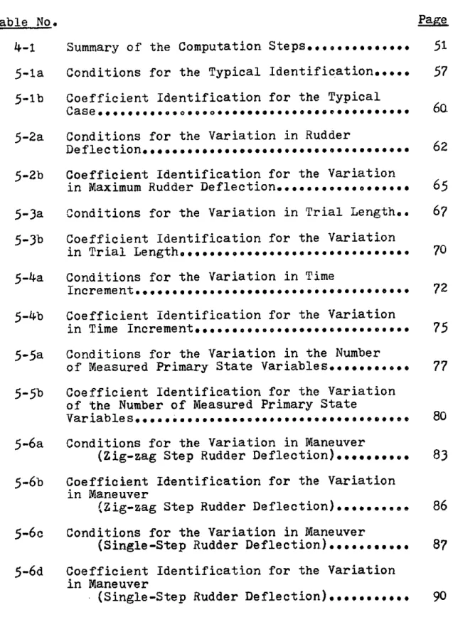
Yv n

is that percentage of the maximum value of the measured output, x. The maximum values are attained from the tra-jectory of the deterministic model (w = v = 0) over the interval of observation.

This definition has several unfortunate aspects which must be kept in mind. In particular, it should be apparent that problems in specification will arise for those maneuvers where the function is not uniform in magnitude, but rather peaks for a short period during the trial. For these cases, the noise present will be specified by the percentage of that maximum value, but will be added to function values substan-tially lower in magnitude over the majority of the period.

Maximum value of g(t) used in g(t) 00 noise generation

Average value over much of the period

t

Fig. 4-1. Imprecision in Noise Definition

In these cases, therefore, the actual noise present during the identification process will be noticably larger than that

specified, possibly by an order of magnitude or more.

4.3 The Identification Process

Much of the actual implementation of the theory developed up to _{this point is described in the Appendix. However, a}

summary of the various steps leading to the results ofthe next chapter should be of value at this time.

The state-space representation of the system was developed in Chapter III and specialized for a surface ship moving with three degrees of freedom. Theoretically, this leads to at least nine primary state variables (x, y ,*, u, v, r,u

v, r, * *) which could be measured during a particular maneuver. In reality this is not the case. Some of these variables can not be recorded at all during full-scale trials, while others require special devises not normally available on-board ship during maneuvers. Those variables which could be readily recorded by traditional methods are

yaw velocity, r, and angle, *, along with the sway acceleration

;, actually (V + ru0) * A general program dealing with nine

primary state variables was developed, but most of the identification studies deal with these three variables

-r, *, and V. Indirectly, the -sway velocity, v, was also incorporated. Use of an integrating accelerometer on-board shp, while not permitting direct measurement of v, would give an indirect record of the sway velocity which could be used in the identification by the filter. Thus, for this

50

study the state vector is defined as,

'v

r

There may be a problem arising from the dependence of v upon the measured acceleration, ;, though in this study it did not become readily apparent.

Equations for each of the primary state variables can be derived from eq. (4.7) - v directly from the definition and v,r and f from the integration of their respective equations. 2 r = vdt ti r =

Irdt

Using these state variables, the remaining steps in the identification process can be summarized as in Table 4-1.

For this study, the noisy data had to be generated within the program itself before it could be processed.

STEP 1: _{Generate the noisy sea-trial data,} B(t)x + w

z Hx + v

STEP 2: Propagate the estimated state and error covariance matrices over one time step,

x=B~t)x ^9 A z = iMx -m

_H

STEP 3: Calculate the Kalman filter gain matrix,

K = EHT (HEHT + R)"

STEP 4: Update the estimated state and error

covariance matrices at the end of the step,

2'

El = E - KHE

STEP 5: Set the updated state and error covariance

matrices as the new estimates and repeat

STEPS 2 through 5 until the end of the

identification process.

Chapter V

RESULTS OF THE IDENTIFICATION PROCESS

The application of the theory developed in Chapters II and III to the problem of identifying the coefficients for a Mariner-class surface vessel was shown in the last chapter.

The equations for the extended Kalman filter were given in Table 4-1 as steps of a procedure for their computation. What remains is for the theory to be tested on the system and see if indeed this technique for systems identification

is valid under the given conditions.

A program was deloped to do these tasks using the MIT IBM 370/168. It is listed in the Appendix, along with a detailed description of it's use and function. The reader

is referred to this section for those details. However, a few brief points are in order at this time.

An attempt was made to keep the program as general as possible, requiring only a change in the input to enact

wholesale alterations in the structure of the identification. For the most part, this was accomplished. There remains

some card shifting to enable the user to select different measured state variables, but for choices in coefficients identified, trial types and lengths and the like, only a variation in the data deck is necessary.