UNIVERSITÉ DE MONTRÉAL
COMPARISON OF ADAPTIVE BEHAVIORS OF AN ANIMAT IN
DIFFERENT MARKOVIAN 2-D ENVIRONMENTS USING XCS CLASSIFIER
SYSTEMS
ARMIN NAJARPOUR-FOROUSHANI DÉPARTEMENT DE GÉNIE ÉLECTRIQUE ÉCOLE POLYTECHNIQUE DE MONTRÉAL
MÉMOIRE PRÉSENTÉ EN VUE DE L’OBTENTION DU DIPLÔME DE MAÎTRISE ÈS SCIENCES APPLIQUÉES
(GÉNIE ÉLECTRIQUE) Juin 2013
UNIVERSITÉ DE MONTRÉAL
ÉCOLE POLYTECHNIQUE DE MONTRÉAL
Ce mémoire intitulé:
COMPARISON OF ADAPTIVE BEHAVIOR OF AN ANIMAT IN DIFFERENT MARKOVIAN 2-D ENVIRONMENTS USING XCS CLASSIFIER SYSTEMS
présenté par : NAJARPOUR-FOROUSHANI Armin
en vue de l’obtention du diplôme de : Maîtrise ès Sciences Appliquées a été dûment accepté par le jury d’examen constitué de :
M. LE NY Jérôme, Ph.D., président
M. BRAULT Jean-Jules, Ph.D., membre et directeur de recherche M. PARTOVI NIA Vahid, Ph.D., membre
DEDICATION
To my parents who taught me hard work To my grandmother for her encouragement
ACKNOWLEDGEMENTS
I would like to express my sincere gratitude to my supervisor of research, Mr Jean-Jules Brault who provided me advices and supervision to successfully complete this project. Thanks to Professor Jerome Le Ny and Professor Vahid Partovi Nia for their helpful guidance and comments on my thesis.
Special thanks to my parents who gave me unconditional love, patience, and encouragement during this work.
RÉSUMÉ
Le mot "Animat" fut introduit par Stewart W. Wilson en 1985 et a rapidement gagné en popularité dans la lignée des conférences SAB (Simulation of Adaptive Behavior: From Animals to Animats) qui se sont tenues entre 1991 à 2010. Comme la signification du terme "animat" a passablement évoluée au cours de ces années, il est important de préciser que nous avons choisi d'étudier l'animat tel que proposée originellement par Wilson.
La recherche sur les animats est un sous-domaine du calcul évolutif, de l'apprentissage machine, du comportement adaptatif et de la vie artificielle. Le but ultime des recherches sur les animats est de construire des animaux artificiels avec des capacités sensorimotrices limitées, mais capables d'adopter un comportement adaptatif pour survivre dans un environnement imprévisible. Différents scénarios d'interaction entre un animat et un environnement donné ont été étudiés et rapportés dans la littérature. Un de ces scénario est de considérer un problème d'animat comme un problème d'apprentissage par renforcement (tel que les processus de décision markovien) et de le résoudre par l'apprentissage de systèmes de classeurs (LCS, Learning Classification Systems) possédant une certaine capacité de généralisation. L'apprentissage d'un système de classification LCS est équivalent à un système qui peut apprendre des chaînes simples de règles en interagissant avec l'environnement et en reçevant diverses récompenses.
Le XCS (eXtended Classification System) introduit par Wilson en 1995 est le LCS le plus populaire actuellement. Il utilise le Q-Learning pour résoudre les problèmes d'affectation de crédit (récompense), et il sépare les variables d'adaptation de l'algorithme génétique de celles reliées au mécanisme d'attribution des récompenses.
Dans notre recherche, nous avons étudié les performances de XCS, et plusieurs de ses variantes, pour gérer un animat explorant différents types d'environnements 2D à la recherche de nourriture. Les environnements 2D traditionnellement nommés WOODS1, WOODS2 et MAZE5 ont été étudiés, de même que des environnements S2DM (Square 2D Maze) que nous avons conçus pour notre étude. Les variantes de XCS sont XCSS (avec l'opérateur "Specify" qui permet de diminuer la portée de certains classificateurs), et XCSG (avec la descente du gradient en fonction des valeurs de prédiction). Nous avons constaté une amélioration sensible de leur performance d'apprentissage.
Nous avons proposé une version combinant XCSS et XCSG, appelée XCSSG. La comparaison des résultats montre que pour des environnements simples tels que WOODS1 et WOODS2, les performances de tous les algorithmes (soit le nombre d'étapes que l'animat doit faire pour atteindre la nourriture) déjà proposés sont très proches, mais que dans des environnements plus complexes tels que MAZE5, l'approche XCSSG converge rapidement près de la solution optimale (nombre minimum d'étapes).
Pour étudier la capacité d'apprentissage de XCS et ses variantes sur une plus grande variété d'environnements (markoviens et non markoviens) que les environnements classiques WOODSx et MAZEy, nous avons conçu un générateur d'environnements S2DM. Les différents algorithmes XCS étudiés ont été testés sur ces environnements et les résultats montrent clairement que les capacités d'apprentissage des différents XCS s'approchent toutes des performances optimales. De plus, une analyse de l'évolution du nombre de classificateurs/règles d'une population a également été faite pour mieux illustrer les capacités de généralisation de chacun des algorithmes XCS. Nous avons finalement proposés trois nouveaux scénario pour étudier les variations de populations de classificateurs des différents XCS. D'abord, un scénario où les ressources se déplacent légèrement. Puis, un scénario compétitif inter-espèces (XCS vs XCSSG) pour le partage d'une ressource commune. Ce scénario est basé sur les équations de Lotka-Volterra et permet de comparer dynamiquement les performances des deux algorithmes. Un troisième scénario a été proposé faisant intervenir un animat ayant des capacités supérieures de vision afin d'étudier la possibilité d'apprendre dans des environnements non-markoviens pour un animat classique, mais markoviens pour un animat moins myope. Les résultats de ce troisième scénario ne sont pas ceux auxquels nous nous attendions. En effet, l'animat n'a pas su profiter de cette supériorité pour améliorer ses performances. C'est pour nous un problème ouvert que nous nous proposons d'explorer dans une nouvelle recherche.
ABSTRACT
The word “Animat” was introduced by Stewart W. Wilson in 1985 and became popular since the SAB line conferences “Simulation of Adaptive Behavior: from Animals to Animats” that were held between 1991 and 2010. Since the use of this word in the scientific literature has fairly evolved over the years, it is important to specify in this thesis that we have chosen to adopt the definition that was originally proposed by Wilson.
The research on animat is a subfield of evolutionary computation, machine learning, adaptive behavior and artificial life. The ultimate goal of animat research is to build artificial animals with limited sensory-motor capabilities but able to behave in an adaptive way to survive in an unknown environment. Different scenarios of interaction between a given animat and a given environment have been studied and reported in the literature. One of the scenarios is to consider animat problems as a reinforcement learning problem (such as a Markov decision processes) and solve it by Learning Classifier Systems (LCS) with certain generalization ability. A Learning classifier system is equivalent to a learning system that can learn simple strings of rules by interacting with the environment and receiving diverse payoffs (rewards).
The XCS (eXtented Classification System) [1], introduced by Wilson in 1995, is the most popular Learning Classifier System at the moment. It uses Q-learning to deal with the problem of credit assignment and it separates the fitness variable for genetic algorithm from those linked to credit assignment mechanisms.
In our research, we have studied XCS performances and many of its variants, to manage an animat exploring different types of 2D environments in search of food. 2D environments traditionally named WOODS1, WOODS 2 and MAZE5 have been studied, as well as several designed S2DM (SQUARE 2D MAZE) environments which we have conceived for our study. The variants of XCS are XCSS (with the Specify operator which allows removing detrimental rules), and XCSG (using gradient descent according to the prediction value).
We have proposed a version combining XCSS and XCSG called XCSSG. The comparison of results shows that for simples environments such as WOODS1 and WOODS2, the performance (the number of steps that the animat must follow to reach the food) of all previously proposed
algorithms are very close, but in more complex environments such as MAZE5, the proposed approach of XCSSG converges rapidly to near optimal solution (minimum number of steps). To investigate the learning ability of XCS and its variants on a higher variety of environments (Markovian or non-Markovian) than the classic environments WOODSx and MAZEy, we have conceived an environment generator S2DM. Different XCS-family algorithms studied have been tested on these environments and the results clearly show the ability of XCS-family in learning all of these new environments and approaching the optimal performances. Furthermore, an analysis of the evolution in the number of classifiers/rules in a population set has also been done to illustrate the ability of XCS-family algorithms in producing general rules (generalization). We have finally presented three new scenarios to study the variations of population sets of different XCS classifiers. First of all, a scenario where resources shift gently. Then, an inter-species competitive scenario (XCS and XCSSG) for sharing of a common resource. This scenario is based on Lotka- Volterra equations and allows to dynamically compare the performances of the two algorithms. A third scenario has been proposed involving an animat with higher vision abilities to investigate the ability to learn in non- Markovian environments for a classic animat but that become Markovians when the animat can perceive on a farther distance. The results of this third scenario are not the ones that we were expecting. Indeed, the animat does not take advantage of its visual superiority to improve its performance. For us it is an open problem that we intend to explore in a new search.
TABLE OF CONTENTS
DEDICATION ... III ACKNOWLEDGEMENTS ... IV RÉSUMÉ ... V ABSTRACT ...VII TABLE OF CONTENTS ... IX LIST OF TABLES ... XIII LIST OF FIGURES ... XIV ABREVIATION ... XXII LISTE OF APPENDICES ... XXIVINTRODUCTION ... 1
CHAPITRE 1 ANIMAT PROBLEM ... 6
1.1 Structure of the animat problem ... 6
1.1.1 Components of an animat problem ... 7
1.2 Choice of the animat problem ... 11
1.3 Wilson’s animat ... 13
1.4 Conclusion ... 15
CHAPITRE 2 REINFORCEMENT LEARNING AND LEARNING CLASSIFIER SYSTEMS ...16
2.1 Reinforcement learning ... 16
2.1.1 Markov chain ... 16
2.1.2 Definition and basic architecture of reinforcement learning ... 17
2.1.3 Temporal differences ... 22
2.2.1 Definition and Introduction ... 23
2.2.2 How does LCS work? ... 24
2.3 Conclusion ... 31
CHAPITRE 3 XCS AND THE ANIMAT PROBLEM ... 32
3.1 XCS :eXtended Classifier Systems ... 32
3.1.1 Introduction ... 32
3.1.2 Description of XCS ... 33
3.1.3 Generalization ... 41
3.1.4 What are the applications of XCS? ... 42
3.2 Animat problem and 2-D environments ... 43
3.2.1 Multi-step problems ... 43
3.2.2 Wilson’s animat problem and 2-D environments ... 43
3.3 XCS animat problem ... 46
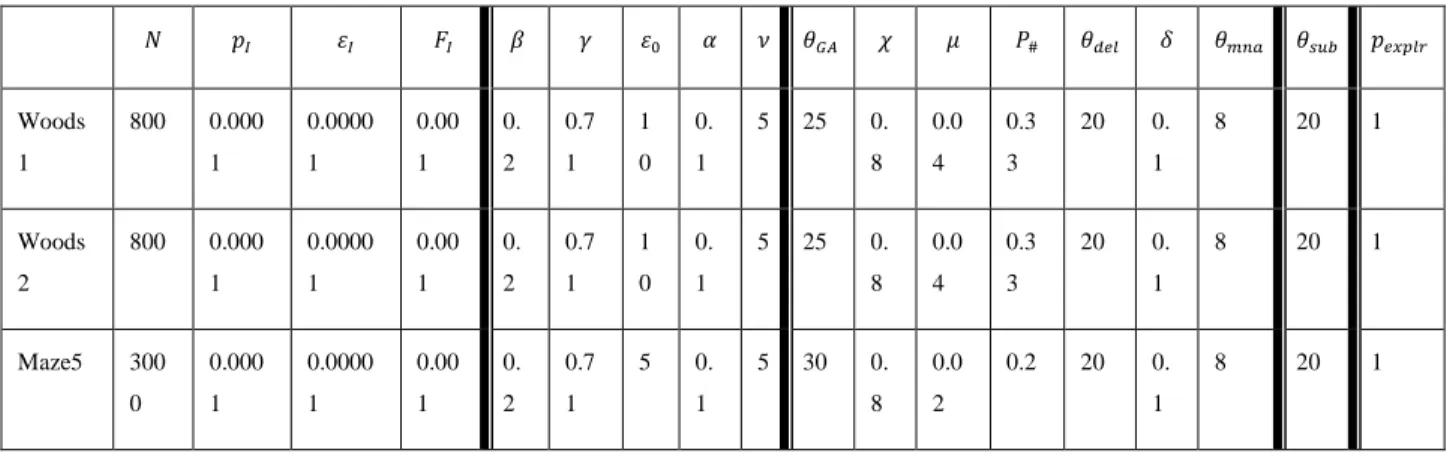
3.4 Experiment ... 47
3.4.1 Experimental setting ... 47
3.4.2 Results for XCS animat in various two-dimensional environments ... 49
3.4.3 Analysis of generalization in XCS ... 57
3.5 A literature review on XCS animat approach ... 58
3.6 Conclusion ... 63
CHAPITRE 4 DEVELOPMENTS IN XCS TO IMPROVE PERFORMANCE IN MARKOVIAN ENVIRONMENTS ... 65
4.1 Introduction to XCSS ... 65
4.1.1 Specify operator ... 65
4.2 Using gradient descent in XCS to improve the performance in Markovian multi-step environments (XCSG) ... 67
4.2.1 Reinforcement learning and XCS ... 67
4.2.2 XCS with gradient descent ... 69
4.3 XCSSG : combination of using Specify operator in gradient-based XCS ... 73
4.4 Results for XCSS, XCSG, and XCSSG in various two-dimensional environments and their comparison ... 74 4.4.1 XCSS ... 75 4.4.2 XCSG direct ... 76 4.4.3 XCSG residual ... 78 4.4.4 XCSSG ... 80 4.5 Comparison of results ... 82 4.6 Conclusion ... 90
CHAPITRE 5 BEYOND THE TRADITIONAL XCS ANIMAT... 91
5.1 Introduction ... 91
5.2 Environment generator and S2DM environments ... 91
5.2.1 Learning results of XCS-family animat in environments 5MS2DM2, 6MS2DM3, 7MS2DM6, 7nMS2DM6, and 7MS2DM8 ... 95
5.3 Unstable resource problem with XCS-animat ... 112
5.4 Interspecific competition problem and XCS animat ... 116
5.4.1 Competitive Lotka-Volterra equation ... 116
5.4.2 XCS-XCSSG competition ... 117
5.4.3 Experimental results ... 119
5.5 An animat with higher vision abilities ... 126
5.6 Comparison of mean and variance in different environments ... 139
5.7 Conclusion ... 142
REFERENCES ... 147 APPENDIX 1- WELL-KNOWN 2-D ENVIRONMENTS ... 153
LIST OF TABLES
Table 3.1: Parameter setting for XCS without subsumption and XCS with subsumption ... 50 Table 4.1: List of parameters for experiment of animat problem with XCSS in each environment ... 75 Table 4.2: List of parameters for experiment of animat problem direct XCSG in each
environment ... 77 Table 4.3: List of parameters for experiment of animat problem with residual XCSG in each
environment ... 79 Table 4.4: List of parameters for experiment of animat problem with residual XCSSG in each
environment. ... 81 Table 5.1:Comparison of Means and Variances in different generated environments. ... 140 Table 5.2: Comparison of Means and Variances in different traditional environments. ... 141 Table 5.3: Comparison of Means and Variances in different Complex-family environments. ... 142
LIST OF FIGURES
Figure 1-1: Basic block diagram of an animat problem. Animat interacts with the environment to
satisfy its needs. ... 7
Figure 1-2: Block diagram of RL animat problem learns by means of payoff from environment. ... 12
Figure 1-3: Block diagram of Wilson’s animat learns by means of payoff from environment ... 14
Figure 1-4: Directions defined for the sensation and the movement of the Wilson’s animat. * is the animat and 0-7 shows the consequence of the sensory vector and also the codes of directions that the animat can move. ... 14
Figure 2-1: block diagram of a reinforcement learning problem. ... 18
Figure 2-2: interaction of LCS with the environment [23]. ... 25
Figure 3-1: A general description of XCS. ... 34
Figure 3-2: Detailed block diagram of XCS; inspired from [24]. ... 35
Figure 3-3: The environment Woods1; inspired from [25] ... 45
Figure 3-4: The environment Woods2; inspired from [1] ... 45
Figure 3-5: maze5 environment; inspired from [26] ... 46
Figure 3-6: Block diagram of a XCS animat ... 47
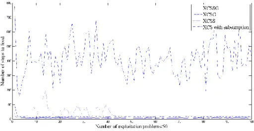
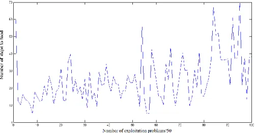
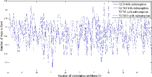
Figure 3-7: XCS animat in woods1 without subsumption, see Figure 3-3. ... 51
Figure 3-8: XCS animat in woods2 without subsumption, see Figure 3-4. ... 51
Figure 3-9: XCS animat in maze5 without subsumption, see Figure 3-5. ... 51
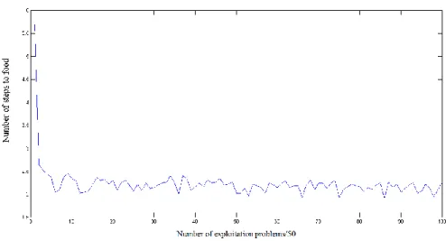
Figure 3-10: XCS animat in woods1 with subsumption. ... 52
Figure 3-11: XCS animat in woods2 with subsumption. ... 52
Figure 3-12: XCS animat in maze5 with subsumption. ... 53
Figure 3-13: XCS animat in woods2 without subsumption for ... 55
Figure 4-2: Block diagram of XCSG. ... 71
Figure 4-3: Block diagram of XCSSG. ... 74
Figure 4-4: XCSS animat in woods1... 75
Figure 4-5: XCSS animat in woods2... 76
Figure 4-6: XCSS animat in maze5... 76
Figure 4-7: XCSG animat in woods1. ... 77
Figure 4-8: XCSG animat in woods2. ... 78
Figure 4-9: XCSG animat in maze5. ... 78
Figure 4-10: Residual XCSG animat in woods1. ... 79
Figure 4-11: Residual XCSG animat in woods2. ... 80
Figure 4-12: Residual XCSG animat in maze5. ... 80
Figure 4-13: XCSSG animat in woods1. ... 81
Figure 4-14: XCSSG animat in woods2. ... 82
Figure 4-15: XCSSG animat in maze5. ... 82
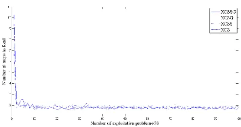
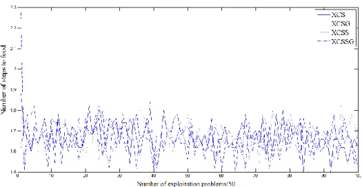
Figure 4-16: Comparison of XCS without subsumption, XCSS, direct XCSG, and XCSSG in woods1. ... 83
Figure 4-17: Comparison of XCS with subsumption, XCSS, direct XCSG, and XCSSG in woods1. ... 83
Figure 4-18: Comparison of XCS without subsumption, XCSS, Residual XCSG, and XCSSG in woods1. ... 84
Figure 4-19: Comparison of XCS without subsumption, XCSS, direct XCSG, and XCSSG in woods2. ... 84
Figure 4-20: Comparison of XCS with subsumption, XCSS, direct XCSG, and XCSSG in woods2. ... 85
Figure 4-21: Comparison of XCS without subsumption, XCSS, Residual XCSG, and XCSSG in woods2. ... 85
Figure 4-22: Comparison of XCS without subsumption, XCSS, direct XCSG, and XCSSG in
maze5. ... 86
Figure 4-23: Comparison of XCS with subsumption, XCSS, direct XCSG, and XCSSG in maze5. ... 86
Figure 4-24: Comparison of XCS without subsumption, XCSS, Residual XCSG, and XCSSG in maze5. ... 87
Figure 4-25: Random moves of animat in woods1 toward a food. ... 88
Figure 4-26: Applying Q-learning algorithm to solve the animat problem in woods1. ... 88
Figure 4-27: Random moves of animat in maze5 toward a food. ... 89
Figure 4-28: Applying Q-learning algorithm to solve the animat problem in maze5. ... 89
Figure 5-1: 5MS2DM2 environment. ... 92
Figure 5-2: 6MS2DM3 environment ... 93
Figure 5-3: 7MS2DM6 environment ... 93
Figure 5-4: 7nMS2DM6 environment ... 94
Figure 5-5: numbered 7nMS2DM6 environment ... 94
Figure 5-6: 7MS2DM8 environment ... 94
Figure 5-7: Comparison of performance of different XCS algorithms in 5MS2DM2. ... 95
Figure 5-8: Comparison of performance of XCS and XCS with subsumption in 5MS2DM2. ... 96
Figure 5-9: Comparison of different XCS algorithms in 5MS2DM2 when the subsumption mechanism is activated. ... 96
Figure 5-10: Comparison of population of classifiers in XCS, XCSG, XCSS, and XCSSG algorithms in 5MS2DM2. ... 97
Figure 5-11: Comparison of population of classifiers in XCS, and XCS with subsumption in 5MS2DM2. ... 97
Figure 5-12: Comparison of population of classifiers in XCS-family algorithms with subsumption in 5MS2DM2. ... 98
Figure 5-13: Comparison of performance of different XCS algorithms in 6MS2DM3. ... 98 Figure 5-14: Comparison of performance of XCS and XCS with subsumption in 6MS2DM3. ... 99 Figure 5-15: Comparison of different XCS algorithms in 6MS2DM3 when the subsumption
mechanism is activated. ... 99 Figure 5-16: Comparison of population of classifiers in XCS, XCSG, XCSS, and XCSSG
algorithms in 6MS2DM3. ... 100 Figure 5-17: Comparison of population of classifiers in XCS, and XCS with subsumption in
6MS2DM3. ... 100 Figure 5-18: Comparison of population of classifiers in XCS-family algorithms with subsumption
in 6MS2DM3. ... 101 Figure 5-19: Comparison of performance of different XCS algorithms in 7MS2DM6. ... 101 Figure 5-20: Comparison of performance of XCS and XCS with subsumption in 7MS2DM6. . 102 Figure 5-21: Comparison of different XCS algorithms in 7MS2DM6 when the subsumption
mechanism is activated. ... 102 Figure 5-22: Comparison of population of classifiers in XCS, XCSG, XCSS, and XCSSG
algorithms in 7MS2DM6. ... 103 Figure 5-23: Comparison of population of classifiers in XCS, and XCS with subsumption in
7MS2DM6. ... 103 Figure 5-24: Comparison of population of classifiers in XCS-family algorithms with subsumption
in 7MS2DM6. ... 104 Figure 5-25: Comparison of performance of different XCS algorithms in 7nMS2DM6. ... 104 Figure 5-26: Comparison of performance of XCS and XCS with subsumption in 7nMS2DM6.105 Figure 5-27: Comparison of different XCS algorithm in 7nMS2DM6 when the subsumption
mechanism is activated. ... 105 Figure 5-28: Comparison of population of classifiers in XCS, XCSG, XCSS, and XCSSG
Figure 5-29: Comparison of population of classifiers in XCS, and XCS with subsumption in 7nMS2DM6. ... 106 Figure 5-30: Comparison of population of classifiers in XCS-family algorithms with subsumption
in 7nMS2DM6. ... 107 Figure 5-31: Performances of XCS-family algorithms in 7MS2DM8. ... 107 Figure 5-32: Comparison of XCS and XCS with subsumption algorithms 7MS2DM8. ... 108 Figure 5-33: Comparison of different XCS algorithm in 7MS2DM8 when the subsumption
mechanism is activated. ... 108 Figure 5-34: Comparison of population of classifiers in XCS, XCSG, XCSS, and XCSSG
algorithms in 7MS2DM8. ... 109 Figure 5-35: Comparison of population of classifiers in XCS, and XCS with subsumption in
7MS2DM8. ... 109 Figure 5-36: Comparison of population of classifiers in XCS-family algorithms with subsumption
in 7MS2DM8. ... 110 Figure 5-37: 7MS2DM6-B environment ... 113 Figure 5-38: Learning in 7MS2DM6-B environment and the optimal performance. ... 113 Figure 5-39: Unstable resource problem in 7MS2DM6 with different XCS-family algorithms
when the food moves toward direction 1. ... 114 Figure 5-40: Unstable resource problem in 7MS2DM6. Comparison between XCS and XCS with
subsumption when the food moves toward direction 1. ... 114 Figure 5-41: Unstable resource problem in 7MS2DM6. Comparison of population sizes. ... 115 Figure 5-42: Unstable resource problem in 7MS2DM6. Comparison of population size between
XCS and XCS with subsumption. ... 115 Figure 5-43: Competition of XCS and XCSSG animats for learning to find food in the
environment. ... 118 Figure 5-44: Change in the population size of two species in 5MS2DM2. ... 120 Figure 5-45: Probability of selecting a XCS animat from the pool in 5MS2DM2. ... 120
Figure 5-46: Performance of a competitive behavior of XCS-XCSSG classifier systems in 5MS2DM2 environment. ... 121 Figure 5-47: Change in the population size of two species in 6MS2DM3. ... 121 Figure 5-48: Probability of selecting a XCS animat from the pool in 6MS2DM3. ... 122 Figure 5-49: Performance of a competitive behavior of XCS-XCSSG classifier systems in
6MS2DM3 environment. ... 122 Figure 5-50: Change in the population size of two species in 7MS2DM6. ... 123 Figure 5-51: Probability of selecting a XCS animat from the pool in 7MS2DM6. ... 123 Figure 5-52: Performance of a competitive behavior of XCS-XCSSG classifier systems in
7MS2DM6 environment. ... 124 Figure 5-53: Change in the population size of two species in 7nMS2DM6. ... 124 Figure 5-54: Probability of selecting a XCS animat from the pool in 7nMS2DM6. ... 125 Figure 5-55: Performance of a competitive behavior of XCS-XCSSG classifier systems in
7nMS2DM6 environment. ... 125 Figure 5-56: 24 cells sensory information. ... 126 Figure 5-57: 10 cells sensory information. ... 127 Figure 5-58: The left hand is Complex1 environment. The right hand is Complex1 environment
that the blank points are numbered. ... 127 Figure 5-59: The left hand is Complex2 environment. The right hand is Complex2 environment
that the blank points are numbered. ... 128 Figure 5-60: The left hand is Complex3 environment. The right hand is Complex3 environment
that the blank points are numbered. ... 128 Figure 5-61: The left hand is Complex4 environment. The right hand is Complex4 environment
that the blank points are numbered. ... 128 Figure 5-62: The left hand is woods101 environment. The right hand is woods101 environment
Figure 5-63: The results of learning of XCS animat with normal vision and higher vision abilities in Complex1 environment. ... 129 Figure 5-64: The population size of classifiers with normal vision and higher vision abilities in
Complex1 environment (XCS). ... 130 Figure 5-65: The results of learning of XCSSG animat with normal vision and higher vision
abilities in Complex1 environment. ... 130 Figure 5-66: The population size of classifiers with normal vision and higher vision abilities in
Complex1 environment (XCSSG). ... 131 Figure 5-67: The results of learning of XCS animat with normal vision and higher vision abilities
in Complex2 environment. ... 131 Figure 5-68: The population size of classifiers with normal vision and higher vision abilities in
Complex2 environment (XCS). ... 132 Figure 5-69: The results of learning of XCSSG animat with normal vision and higher vision
abilities in Complex2 environment. ... 132 Figure 5-70: The population size of classifiers with normal vision and higher vision abilities in
Complex2 environment (XCSSG). ... 133 Figure 5-71: The results of learning of XCS animat with normal vision and higher vision abilities
in Complex3 environment. ... 133 Figure 5-72: The population size of classifiers with normal vision and higher vision abilities in
Complex3 environment (XCS). ... 134 Figure 5-73: The results of learning of XCSSG animat with normal vision and higher vision
abilities in Complex3 environment. ... 134 Figure 5-74: The population size of classifiers with normal vision and higher vision abilities in
Complex3 environment (XCSSG). ... 135 Figure 5-75: The results of learning of XCS animat with normal vision and higher vision abilities
Figure 5-76: The population size of classifiers with normal vision and higher vision abilities in Complex4 environment (XCS). ... 136 Figure 5-77: The results of learning of XCSSG animat with normal vision and higher vision
abilities in Complex4 environment. ... 136 Figure 5-78: The population size of classifiers with normal vision and higher vision abilities in
Complex4 environment (XCSSG). ... 137 Figure 5-79: The results of learning of XCS animat with normal vision and higher vision abilities
in woods101 environment. ... 137 Figure 5-80: The population size of classifiers with normal vision and higher vision abilities in
woods101 environment (XCS). ... 138 Figure 5-81: The results of learning of XCSSG animat with normal vision and higher vision
abilities in woods101 environment. ... 138 Figure 5-82: The population size of classifiers with normal vision and higher vision abilities in
ABREVIATION
AB Adaptive Behavior
ACS Anticipatory Classifier Systems AI Artificial Intelligence
Alife Artificial Life
ARP Action Reply Process CAS Complex Adaptive Systems CXCS Corporate XCS
GA Genetic Algorithm
GP Genetic Programming
LCS Learning Classifier Systems MDP Markov Decision Process NSF Number of Steps to Food RL Reinforcement Learning SB-XCS Strength-based XCS
XCS EXtended Classifier Systems XCSF XCS for function approximation XCSG Gradient-Based XCS
XCSI XCS for integer inputs
XCS-LP XCS with continuous reinforcement XCSM XCS with addition of Memory XCSS XCS with Specify
XCSSG Gradient-based XCS with Specify
ZCS Zeroth-level classifier systems S2DM Square 2 Dimensional Maze
LISTE OF APPENDICES
INTRODUCTION
Motivation
The concept of “Animat” was invented by Stewart W. Wilson in 1985 by publishing the paper “KNOWLEDGE GROWTH IN AN ARTIFICIAL ANIMAL [2].” Using this word became popular after conference “Simulation of adaptive behavior: from animals to animats (SAB90)” in 1990 in Paris. After three conferences, the International Society for Adaptive Behaviour was formed that contains many contributions related to the animat approach. They have a journal, Adaptive Behaviour and a proceeding which is published every two years.
In debates about artificial intelligence, several researchers believed that recreating the human intelligence as a purpose is a very far and doubtful goal, and it would be better to first understand basics and simpler capacities of intelligence that are common between human and animals while interacting with the environment, such as their adaptive behavior for foraging, navigation and obstacle avoidance. According to these debates two important things were considered: inspiration from biology and applying the bottom-up approach to AI (Artificial Intelligence). Wilson suggested using of animal models of increasing complexity and synthesize them to study natural and artificial intelligence [2]. Using the animal models to study intelligence depending on the complexity of the model or complexity of the animal can lead to intelligence at its primitive levels or more complex levels such as human. The primitive animal models give a good insight into the basis of intelligence in general. They solve basic problems which are common among a wide range of animals from the simplest ones such as C. elegans to the most complex ones such as human being. The behavioral models of simple animals are based on solving these problems. These behavioral models help us to understand the whole intelligence and design more complex models.
Based on [2] the simple animals have four common basic characteristics:
1. Animals at each moment receive only some sensory signals from the environment which are important at that moment.
3. Existence or absence of certain signals such as food consumption has special meaning for animals.
4. Animals act to optimize the rate of occurrence of certain signals. This action is produced by an internal and external operation.
1 and 2 are related to sensory-motor system of animals and 3 and 4 are related to the notion of “need”. Wilson called the artificial animals that follow these four rules “animat”.
Animat Approach
The animat approach is sub-category of evolutionary computation, machine learning, adaptive behavior, and artificial life. Artificial life or Alife investigates the logic and formal basis of life and living systems to understand the complex information processing in these systems and tries to simulate or synthesize based on these bases. Emergent property is central to alife research. It is a property that a system and its properties (a “whole”) as the interaction of its parts has a global behavior that can’t be understood of its parts [3]. Actually, alife focuses on those complex systems that are inspired from life [4]. Alife is a bottom-up (synthetic) approach constructing life from its basic elements. Adaptive behavior is the behaviour in a changing and unknown environment for survival that can change in response to agent’s environment [5].
Animats are artificial animals. They can be simulated animals or physical robots. The definition of the animat approach is:
Understanding the formal basis of animals’ life and synthesize it in a form of an artificial animal in a changing and uncertain environment to provide understanding of adaptive behavior of animals for surviving in artificial and real world.
Life of animat is considered as its adaptive behaviour which is the interaction between animat and the environment for surviving, thus, environmental complexity has effect on the adaptive behavior of the animat. Complex adaptive behaviors are the result of complex environments. So, a general model of interaction between agent (animat) and environment needs a general theory of environment. Wilson in [6] introduced a general theory of environment based on finite state
machines. The general theory of environment can be a dynamic system model too, i.e. the behavior of agent in an environment is a dynamic system, where a state is the condition of animat at a given time and its dynamic determines the state change [7]. Two capabilities are central to animat approach: sensing the environment and action. These abilities together are considered a sensory-motor system. Animats search for essential sensory information and select actions to perform beneficially in the environment [3]. Sensory system links the agent to environment and actions allow it to behave adaptively [5]. Adaptive behavior is the consequence of actions that animat performs based on the sensory information from the environment and application of a control algorithm (control architecture). Needs are the main drivers of animal behavior and can be regarded the root of intelligence. The concept of needs is common from human to very simple animals, i.e. all of them have a number of needs. To satisfy needs animat has to live in the environment and the complexity of environment influences the complexity of its behavior and the performance of its operation.
The long-term goal of animat approach is to understand human intelligence incrementally, i.e. starting from simple environments and increasing the complexity of environments and architectures by adding necessary features (bottom-up approach). The meaning of “incrementally” is increasing the complexity of needs or complexity of environment to determine change in the animat behavior necessary to satisfy the needs [6].
Animat Approach and AI
AI is the synthetic and computational study of intelligence. AI includes two approaches to deal with the problems of agent behaving in the environment: standard AI and Behavior-based AI. Standard AI concerns with the competition of machine with human by simulation of the abilities of human cognition in the form of computer programs that are connection of symbols in internal reasoning that yield external stimuli [6]. Standard AI was popular until near 1990. In behavior-based AI agent interacts with the environment through sensing and making action.
The behavior-based AI emerged against the limitations of the standard AI in which uses symbol-based tasks and ignores sensory information, needs, perception, adaptation, learning, and coping with the environment. The standard AI is limited for controlling of a physical agent in an environment and has a big processing delay when interacts with an unknown environment, and therefore, it is limited for understanding of intelligence.
The animat approach is a behavior-based approach which considers interaction with the environment through sensing and action. Its aim is to simulate and understand complete animal-like systems at simple level and reach to human intelligence “from below” incrementally.
Reinforcement learning description of the animat problem
Animat problem can be described in several ways. One way is the problem of an animat in the environment containing payoff (reward or punishment) that are given to each action that animat performs. In this kind of problem the animat tries to learn and maximize its total reward by searching the environment. Among several methods to solve a reinforcement learning problem, learning classifier systems have the ability of generalization (ability of the system to reach to a rule for assigning of each action to each state more general than having a table for assignment of actions to all states). Learning classifier systems learn the payoff environment by a set of rules called classifiers. Among different learning classifier system methods, XCS that was introduced by Wilson (1995) is the most popular and has better performance and generalization ability in comparison to the other learning classifier systems methods. Animat problems can be represented in a framework to be solved with XCS classifier systems. The developed models of XCS for more complex Markovian environments are XCS-with-Specify (XCSS) and gradient-based XCS (XCSG). XCSS removes rules with mal-functionalities and XCSG presents a gradient-based prediction of reward to improve the performance of XCS.
Objectives
The objective of this thesis is to solve a reinforcement learning-based animat problem using XCS classifier systems and compare the performance in different 2-D environments. The contribution of this work is the presentation of a new method that is a combination of XCS-with-Specify operator (XCSS) and gradient-based XCS (XCSG) that is called XCSSG to improve the performance and speed of the system. A comparison between performance of several developed models of XCS such as XCS, XCSS, XCSG, residual XCSG, and XCSSG is done in this thesis. Study of the effect of the subsumption mechanism (a mechanism that removes useless rules of the system) on the performance of XCS in various Wilson’s animat problems in different environments is also presented. Other contributions of this work are introducing new maze environments beyond the traditional environments that are presented in the literature and trying to solve them using XCS-family algorithms (XCS, XCSG, XCSS, XCSSG, XCS with
subsumption). Introducing an unstable resource problem with XCS animat to test the ability of XCS to adapt to a changing environment is presented in this work. A competitive platform for comparison of XCS and XCSSG is introduced based on Lotka-Volterra equation to introduce new way for comparison of two adaptive algorithms. An animat with higher vision abilities is also introduced in this thesis to provide conditions to convert a non-Markovian environment to a Markovian environment for the animat and let XCS and XCSSG to learn with these new sensory abilities. In Chapter 1 first the animat problem and its basic components are described and Wilson’s animat that is a particular kind of reinforcement learning (RL) animat will be introduced. It is followed in Chapter 2 by providing an introduction to the mathematical description of a reinforcement learning problem, methods to solve it, and description of learning classifier systems. In Chapter 3 XCS is introduced as the main method in this thesis to deal with the Wilson’s animat problem and it finishes by a literature review on XCS animat. To use XCS in more complex environments and improve its performance, XCSS, XCSG, and their combination (XCSSG) are introduced in Chapter 4. At the end of this chapter a comparison of different methods and also their comparison with Q-learning are made to compare the work with the older basic methods. To study the abilities of XCS beyond the traditional works on XCS, in Chapter 5 new environments are presented and new scenarios are introduced to test the ability of the XCS animat in operating in new situations. Results of learning XCS are then compared and conclusions are presented.
CHAPITRE 1
ANIMAT PROBLEM
In this chapter the basic components of animat problem and the role of each component are introduced. The concept of Reinforcement learning animat and Wilson’s animat are introduced and used as the basis of animat problem in this thesis.
1.1 Structure of the animat problem
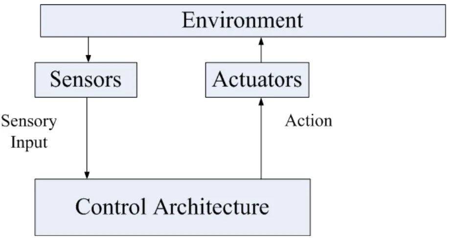
Animat problem is a problem that is expressed based the formal basis of animals’ life in which an agent interacts adaptively with an unknown environment to survive. Formal basis of animals’ life differs for different animals. However, there are basic rules that are common between all of them, from the simplest one to human intelligence and are considered as the basic rules of intelligence in animals. These basic rules are categorized into two groups: 1) having sensory-motor system and 2) having needs. These two properties construct the common basis of animat problem. Sensory and motor systems are connected by a control architecture that in its simplest form is a reflex, but can perform a more complex functionality such as learning or evolution. Control architecture connects sensing and action by a mapping for the purpose of surviving (e.g. food seeking). Interaction of animat and environment for survival has its root in satisfaction of needs. Depending on the needs that have been considered in an animat problem, environment can be different and the corresponding surviving task to satisfy these needs is different. For example finding food, avoiding obstacles, and wall tracking are various kinds of surviving tasks that are different for different environments. Animat interacts with the environment through sensing and action to satisfy its needs. Adaptive behavior is the result of interaction between animat and environment. An abstract diagram representing the basic architecture of animat problem is shown in Figure 1-1.
Long term goal of the animat approach is bottom-up understanding of intelligence that is starting from primary levels of intelligence (simple animals with minimal architecture in simple environments) and increasing complexity of problem until reaching to human intelligence. So, more components can be added to the basic architecture of the animat problem to make it appropriate for more complex environments.
Figure 1-1: Basic block diagram of an animat problem. Animat interacts with the environment to satisfy its needs.
1.1.1 Components of an animat problem
Based on the definition of the animat problem the basic components of an animat problem are as follows:
- Formal basis of animals’ life - Environment
- Adaptive behavior
Formal basis of animals’ life are the bio-inspired rules based on real rules of the life of animals
and describing the life of an animat and its interaction with the environment. Formal basis of animals’ life are usually general rules that are common between all types of animals from the simplest one such as fruit fly to the most complex one such as human. These bases are classified into two main groups that are common among every kind of animals: i) having sensory-motor system and ii) having needs. Sensory-motor system consists of sensors to sense the environment and actuators to do action and change sensory signals. Control architecture maps sensory information to the action. This mapping can be a simple reflex or a more complex mapping such as learning. The animat interacts with the environment to satisfy its needs (present or future). This interaction is via the sensory-motor system and the objects that satisfy its needs and are available in the environment. The Animat can be a physical robot or simulated animal in the environment. The body, number and position and type of sensors, number and position and type
of actuators, and the way of connection of these components to the control architecture are significant for the adaptive process. In addition the constraints that are regarded on the animat’s body such as the type of legs or the shape of body can affect the adaptive behavior. So, the word of “embodied” is applied when role of the body is considered important for the adaptive behavior.
Environment is a physical or simulated world containing food or other objects necessary for the
need satisfaction (survival). The environment mainly is the simulation of animals’ ecosystem and is created by inspiration from real ecosystem. Based on the animat’s needs that are regarded for a specific problem an environment is designed and the surviving tasks are assigned. Examples of surviving tasks in various animat problems are acquiring maximum resources of food, reaching to a particular cell, reaching to the first food, maintaining minimum level of energy, living as long as possible, foraging (food seeking), prey hunting, and obstacle avoidance.
Complexity of the environment can be characterized by setting of tasks and its pattern of objects. For example distribution of food (in foraging task) and obstacles determines the complexity of surviving task for some kind of animat problems. So, a formal theory of environment can be used to give a better insight into the complexity of environment. A formal theory of environment can be expressed by a finite state machine (FSM) model [6]. In this model actions are input to the environment and sensory stimuli are output. For a given input the number of possible outputs is finite. The model is expressed by:
Where is the action, is the sensory stimulus, is the current state of the perceived
environment, and is discrete time. is a function that represents the change of state of the environment to the next state (transition function) for action at time-step and is a function that represents the sensory stimulus at state for action at time-step . The model says that the action in an environment results a new sensory stimuli. It also can be concluded that the same action inputs to different situations of the environment result in different sensory stimuli. This model is also used to provide a measure for the level of complexity [6]. If the animat is equipped
with more sensors in a certain environment, it can see more details of the environment and may adapt easier.
Two classes of environments based on the state transition of an agent (that is situated in the environment) are definable: Markovian environments and non-Markovian environments. Markovian environments are those environments that the best action in a state can be determined by having the sensory information in current state. Non-Markovian environments are environments that the best action in a state is not determinable only from the sensation vector in current state. In other words, for non-Markovian decision process information from the states that it has passed before, or may be all of them are needed.
Adaptive behavior is the result of internal cognitive process of animat and its interaction with
the environment [8]. It is a behavior for need satisfaction (surviving) in an unknown environment. The surviving of animat depends on the ability of animat to cope with the environment through experience. This ability is different depends on the complexity of environment, the surviving task that is based on the regarded needs, the control architecture, number, position, and type of sensors and actuators. Control architecture has a central role in the adaptive behavior. It maps sensory information to the action and the sequence of actions constructs the adaptive behavior of animat. Based on [3] and [9], [10], and [11] different kinds of control architectures (adaptive behaviors) are as follows:
1. Programmed behavior :
Programmed behavior is the result of a control architecture that is designed for a certain purpose. For example, in a population of animats all of them can have the same architecture and the architecture has been constructed from several layers each composed of networks of finite state machine. This kind of architecture is designed to decompose complicated architectures into simple modules each perform a simple behavior. The modules are organized in different layers that each layer implements a certain goal of agent. Higher layers are more abstract and work to reach to the overall goal. This approach is a bottom-up approach. The programmed behavior can be used for blind robots that operate without sensory information from the environment.
2. Learning:
Learning is the process of building a general model based on a set of seen examples and using that model for prediction in new unseen situations. Importance of learning is in its application to noisy, changing, and unknown environments where animat has to decide what to do in new situations in the environment. In learning animat obtains knowledge by direct interaction to the environment via sensors [12]. Based on the literature three important learning techniques for animat are as follows:
- Unsupervised Learning: is a kind of learning that agent (or animat) learns and
reconstruct patterns by associating different parts of the pattern with the other parts. For example using Kohonen neural network, a robot would be able to recognize different structures of the environments by finding the similarities that it uses to cluster. So, in this way the robot can move in the environment and categorize it. - Reinforcement Learning: learning to behave by receiving payoff from the
environment and trying to maximize the total amount of expected payoff. An environment for animat problem can be accounted as a reinforcement learning problem which animat tries to learn. For example, Markovian environments are formulated as a Markov Decision Process (see 2.1.2.3) that is in fact a reinforcement learning problem. To solve a reinforcement learning problem several techniques such as dynamic programming, temporal difference, Q-learning, bucket brigade algorithm, and as we will see learning classifier systems can be applied.
- Associative Learning: in associative learning animat makes a cognitive map of the environment. Cognitive map is a map that animat memorizes. This map associates the sensory information to actions for the navigation task. For animals the cognitive maps contain topological and metric information about the environment that they have learned to determine. The spatial representation of the environment is encoded in their hippocampus which is part of the animals’ brain to help them survive in the environment.
- Conditioning: a number of learning processes that improve perception or motor skills in animals by perception without need for higher cognitive processes.
3. Evolution:
Evolution is the process of improving behavior of individuals in a population. The improvement performs by selecting the individuals that have been adapted and removing individuals that have not been adapted well. With a simple evolutionary rule it can generate an unpredictable or very complex behaviour that is not planned [13]. The evolution often is based on natural selection models. For animat problem evolutionary strategies that are usually applied are genetic algorithm, genetic programming, evolving control parameters of neural networks with GA or GP, evolution of control program, evolutionary programming, and evolution strategies.
4. Development:
In artificial evolution the genotype of an individual is decoded and transformed into a phenotype. In nature, interaction of genetic information and environment builds the phenotype of an animal. This process is called development and here a bio-inspired developmental architecture can be considered for animat. In development architectures connections between sensory and motors neurons is possible. The structure and function of these neurons are designed by human. Geometrical nature of the developmental system and the animat’s body is important to build and connect neural modules. The development architecture has been used to evolve a neural network to control the locomotion of a 6-legged animat[14].
5. Combination of different forms of control architectures is possible. Examples are as follows: - Evolution based learning techniques
- Evolution of neural controller
- Neural controllers that are built incrementally at run time using RL techniques - Recurrent neural networks learning using back-propagation
- Self-organizing neural networks.
1.2 Choice of the animat problem
Research in the animat context can be performed on problem as a whole with consideration of all details or can be focused more on one specific component. Subject of different researches in animat context based on [15] are: Adaptive behavior, Perception and motor control, Architecture,
Action selection and behavioral sequences, Internal world model for navigation, Learning, Evolution, External environment, Collective and social behaviors, and Applied adaptive behavior. Depending on the considered details in each subject a variety of tasks and problems are available. So, it is clear that the animat problem can be represented in different ways.
One of way for representation of animat problem is reinforcement learning approach.
Reinforcement learning (RL) is a form of machine learning, in which an agent operates in the
environment by receiving reward. The final goal of agent is maximization of the total rewards. The animat problem in this way can be expressed in the RL framework: action, sensing the environment, state, and reward (such as obtaining a food or reaching to an obstacle).
In RL context, environment can be Markovian, non-Markovian, or any combination of them. The definition of environment in reinforcement learning depends on the important features that are considered in a certain problem. In the case of Markovian environments RL problem is expressed as a Markov decision process. For Markovian environments Q-learning (see 2.1.3.1), learning classifier systems, and dynamic programming methods can be used in different ways for an animat to survive. For non-Markovian problems there is no exact method to solve. We call the animat problem that is represented in the reinforcement learning framework “RL animat”. The block diagram of a typical RL animat is shown in Figure 1-2.
Figure 1-2: Block diagram of RL animat problem learns by means of payoff from environment. Learning classifier systems (LCS) have generalization capability and are applicable for large and complex problems where Q-learning alone cannot be used because it needs a high amount of
memory and doesn’t have generalization ability. For this reason, in this project LCS is applied to deal with the animat problem. We call “LCS animat” or “Wilson’s animat” to refer to a RL animat problem that LCS is used as its control architecture.
1.3 Wilson’s animat
Wilson studied learning of animat in the environment using learning classifier systems that is a specific type of RL animat problem [2]. The block diagram of Wilson’s animat is illustrated in Figure 1-3. It is specific type of RL animat that the control architecture is a learning classifier systems algorithm. The environment that he considered for the animat was a rectangle with 18 rows and 58 columns that was continued toroidally at the edges and was called woods7 [2] (see Appendix-1). In woods7 at various positions there exist objects which are represented by and and in which s are obstacles, s are foods, and s are empty places. At each position animat senses 8 cells around it and stores them in a sense vector which is clockwise representation of these positions starting from the top. This vector is composed of s, s, and s. For each of these objects an internal two bits representation is considered, 11 for F, 01 for T, and 00 for b. So, a 16 bit sense vector represents the animat’s sensory information at each time step. This 16 bits sense vector is called the detector vector. For example . Detector vector will be used as the input for the process of LCS control architecture in animat. A number between 0-7 which represents one step movement to one of the 8 available directions is considered as an action. The action numbers are constructed clockwise starting from the top (see Figure 1-4). The movement is toward a position which may contain an object. If the movement is toward 00, the animat will receive no signal. If the movement is toward 01, the step won’t be allowed because it’s an obstacle. If the movement is toward 11, the animat will receive a reward signal. The goal of Wilson’s animat is learning to find a food, i.e. after finding a food the process starts again from a random blank point in the environment and after a lot of iterations from different starting points, the number of steps to food reduces to a stable value. Wilson made a reinforcement learning model of animat problem and solved it using learning classifier systems (LCS). The LCS mechanism uses the reward from the environment. So, at each step that the animat eats a food; a reward is given to him that is used in the LCS mechanism.
Figure 1-3: Block diagram of Wilson’s animat learns by means of payoff from environment
Figure 1-4: Directions defined for the sensation and the movement of the Wilson’s animat. * is the animat and 0-7 shows the consequence of the sensory vector and also the codes of directions that the animat can move.
In learning classifier systems the association between sensing and action is represented by condition-action rules. The condition matches the aspects of local environment and the internal state and action determine the internal state. This association are learned by the animat. The basic problem of LCS animat is the generation of the rules to take an appropriate action to optimize the rate of occurrence of certain signals. So, the first step is rule discovery, second step is keeping the rules that work and get rid the rules that don’t work, and third step is generalization of the kept rules [2].
1.4 Conclusion
In this chapter the concept of animat problem and its components were introduced. It was shown that animat should perform adaptive behavior to survive and the control architecture has a central role toward this purpose. Different approaches to animat problem also were described and it was shown that one of the main approaches is the RL animat that the architecture of animat problem is matched with a reinforcement learning problem. For this project Wilson’s animat that is a specific kind of RL animat is studied. The basis of Wilson’s animat are similar to the original animat in [2] but the choice of environments and the algorithms of learning are more precise. There are many different LCS algorithms, but the most well-known and popular one is XCS classifier systems that is chosen and is studied in detail in Chapter 3. So, the purpose of this thesis is to solve and learn Wilson’s animat problem to survive in different 2-D environments with several kinds of XCS classifier systems in different situations and scenarios. In the next chapter reinforcement learning and learning classifier systems are introduced.
CHAPITRE 2
REINFORCEMENT LEARNING AND LEARNING
CLASSIFIER SYSTEMS
In the previous chapter the definition of animat problem and its structure were presented. It was stated that the adaptive behavior is essential for survival task. The adaptive behavior can be modeled by a reinforcement learning model that animat learns to survive by receiving payoff from the environment. The focus of this thesis is on Wilson’s animat that is a specific class of reinforcement learning animat problems. To make a mathematical expression for the Wilson’s animat problem in this section Reinforcement Learning (RL) and Learning Classifier Systems (LCS) frameworks are introduced.
2.1 Reinforcement learning
2.1.1 Markov chain
A Markov process is a stochastic process in which each state depends only on the previous state. Markov chain is a Markov process which has discrete and countable number of states and operates in discrete time. Suppose that is a random variable and is the value of random variable at time . is a state space which is the values that can take at discrete times. The random variable is a Markov chain if:
It shows that the next state of random variable (Markov chain) only depends on the current
state . Markov chain is a chain starting with which is: . A probability is the probability of going from to by one step and called transition probability. A Markov chain can be expressed based on transition probabilities. The mathematical expression of transition probabilities is:
Let’s denote as the probability that the chain is in state at time and denote . The dimension of is the same as dimension . The chain will start with . All of the elements of are 0 except
one of them which the random variable is in that state. From Chapman-Kolmogrov equation we can write:
The probability transition matrix is denoted by that elements are . On the other hand sum of the rows elements of are one ( ). Hence, and so .
-step transition probability is the probability of starting from state and after steps
reaching to state after states.
Where is the element of .
A Markov chain may reach a stationary distribution , where the state and after that next states are independent of initial condition. So, we will have:
is left eigenvector associated with the eigenvalue of [16].
2.1.2 Definition and basic architecture of reinforcement learning
Reinforcement learning is learning based on maximization of reward for agent that performs in an environment. The idea of reinforcement learning is inspired from study of the behaviour of animals from psychological point of view. Animals or human many times do a lot of works without receiving any reward to reach to a later reward at the end. So, reinforcement learning is based on this idea [17]. For example in foraging, an animal does a lot of actions in search for food and the obtained food is a reward, actually this is a distant reward. In reinforcement learning finding food has a positive reward and motions that consume energy have negative reward or punishment. Reinforcement learning builds a computational model of this type for complex behaviour of animals. In reinforcement learning the role of environment is important because the agent can’t act only based on some pre-defined rules in a changing environment and it should
change its action adaptively. Applications of reinforcement learning are in robotics, animals’ behaviour, games, control theory and finance.
2.1.2.1 Architecture of reinforcement learning
Figure 1-1simply shows the architecture of reinforcement learning:
Figure 2-1: block diagram of a reinforcement learning problem.
In this diagram the agent first observes the environment that is the current state of the environment and then chooses an action and applies it to the environment. In the next step he receives an immediate reward from the environment for his action. The goal of agent is to maximize sum of the rewards. Agent should learn how to choose actions to obtain maximum sum of the rewards. It tries various actions in some states and after several times, learns which action is the best for which state. So, the agent in fact finds a policy (the rule of choosing an action at each state of the environment). There are methods in reinforcement learning which agent without predicting the effect of its action on the future rewards can learn optimal policy.
2.1.2.2 Problem statement
An agent in the environment, moves in discrete time steps denoted by : and at each time step the agent observes the state of environment (that can be considered as the state of agent too) where is the set of possible states. According to the observed state, the agent
chooses an action where is the set of possible actions that can be chosen at state . In the next step the agent will receive reward when it is in state .
At each time step in each state, the agent chooses an action from . It is a type of probabilistic mapping that is called policy and is denoted by . It represents the probability that if . An agent tries to change the policy for the purpose of maximum return (total rewards) in long sense. The agent selects actions to maximize the function:
is time step and the factor is discount factor which determines the importance of later and sooner rewards. For it is called episodic task.
2.1.2.3 Reinforcement learning in Markovian environments
The environment in which reinforcement learning tries to learn can be a Markovian environment or a non-Markovian environment with different levels of complexity for each one. For example, woods1 is a Markovian environment with eight obstacles and one food, woods101 is a non-Markovian maze environment with closed walls and low level of complexity and woods7 is a non-Markovian environment with a high variety of sensory patterns and high level of complexity (see Appendix 1). The number of similar cells in a non-Markovian environment determines its complexity. Actually, the environment is a problem that agent tries to solve. A Markovian environment in the architecture of reinforcement learning leads to a Markov decision process. This kind of reinforcement learning is called reinforcement learning in Markovian environments. A Markov decision process (MDP) satisfies:
In fact, Markov decision process is the extension of Markov chain when action and rewards are considered. The probability space is the set of different states of the environment (e.g. sensory states).
To make a mathematical expression of a reinforcement learning problem in Markovian environments transition probability and expected value of the next reward are defined as follows:
Transition probability is the probability that the state changes from to given action . The expected value of the next reward is the average of receiving reward in changing from state to with action . , specify the dynamic of a finite MDP (MDP with finite number of states and actions).
(Note that the definitions of conditional probability and conditional expectation value are and .)
2.1.2.4 Policy
Policy is a mapping from state to action at each time step and is denoted by that is probability of when . The agent changes the policy to maximize the return in long sense. To represent change of the policy for the maximum return two functions can be used:
state-value function and action-value function. a) State-value function
State-value function is the value of state under policy :
can be written in a recursive form:
This equation is called Bellman equation and is a unique solution for its Bellman equation [18].
To reach to the purpose of reinforcement learning (maximization of the return function) one should find a policy that maximizes the value function. In MDP, this policy is called optimal policy and is denoted by . The optimal policy is not unique. The maximum state-value function is called optimal state-value function .
b) Action-value function
Another useful function is which is the value of taking action in state under policy :
This optimal policy gives an optimal action-value function :
can be written in terms of :
The Bellman equation for is called Bellman optimality equation and can be written as:
So, the Bellman optimality equation for is:
For finite MDP, Bellman optimality equation has a unique solution that is independent of policy. This solution is composed of solutions according to unknown states. If , are available, the Bellman optimality equation can be solved for , . The purpose in reinforcement learning is to find to maximize or [18].
There are at least two methods to solve this optimization problem: Dynamic programming and temporal difference learning. Dynamic programming is used for conditions when we know the model of environment i.e. the transition matrices and expected rewards. But temporal difference is used when we don’t know transition matrices and expected rewards. So, temporal difference learning methods are more general and useful for higher variety of problems. In the next section we introduce temporal difference methods.