MAppleT: simulation of apple tree development using mixed stochastic and biomechanical models

HAL Id: hal-00831809

https://hal.inria.fr/hal-00831809

HAL is a multi-disciplinary open access archive for the deposit and dissemination of sci-entific research documents, whether they are pub-lished or not. The documents may come from teaching and research institutions in France or abroad, or from public or private research centers.

L’archive ouverte pluridisciplinaire HAL, est destinée au dépôt et à la diffusion de documents scientifiques de niveau recherche, publiés ou non, émanant des établissements d’enseignement et de recherche français ou étrangers, des laboratoires publics ou privés.

MAppleT: simulation of apple tree development using

mixed stochastic and biomechanical models

Evelyne Costes, Colin Smith, Michael Renton, Yann Guédon, Premyslaw

Prusinkiewicz, Christophe Godin

To cite this version:

Evelyne Costes, Colin Smith, Michael Renton, Yann Guédon, Premyslaw Prusinkiewicz, et al.. MAp-pleT: simulation of apple tree development using mixed stochastic and biomechanical models. Func-tional Plant Biology, CSIRO Publishing, 2008, 35 (10), pp.936-950. �hal-00831809�

MAppleT: Simulation of Apple Tree Development Using Mixed Stochastic and Biomechanical Models

Evelyne CostesA, F, Colin SmithA, Michael RentonDB, Yann GuédonB, C, Przemyslaw PrusinkiewiczE and Christophe GodinB,C

A

INRA, UMR 1098 CIRAD-INRA-SupAgro-UM2, 2 Place Viala, 34060 Montpellier, France

B

CIRAD, UMR 1098 CIRAD-INRA-SupAgro-UM2, Avenue Agropolis, TA A-96/02, 34398 Montpellier, France

C

INRIA, Equipe Virtual Plants, Avenue Agropolis, TA A-96/02, 34398 Montpellier, France

D

Department of Agriculture and Food of Western, 35 Stirling Highway, Crawley WA 6009, Australia

E

Department of Computer Science, University of Calgary, Alberta, T2N 1N4, Canada

F

Corresponding author. e-mail: [email protected]

Abstract

Construction of architectural databases over years is time consuming and cannot easily capture the event dynamics, especially when both tree topology and geometry are considered. The present project aimed to bring together models of topology and geometry in a single simulation such that the architecture of an apple tree may emerge from process interactions. This integration was performed using L-systems. A mixed approach was developed based on stochastic models to simulate plant topology and mechanistic model for the geometry. The succession of growth units (GUs) along axes and their branching structure were jointly modeled by a hierarchical hidden Markov model. A biomechanical model, derived from previous studies, was used to calculate stem form at the metamer scale, taking into account the intra-year dynamics of primary, secondary and fruit growth. Outputs consist of 3D mock-ups geometric models representing the progression of tree form over time. To asses these models, a sensitivity analysis was performed and descriptors were compared between simulated and digitized trees, including the total number of GUs in the entire tree, descriptors of shoot geometry (basal diameter, length), and descriptors of axis geometry (inclination, curvature). In conclusion, in spite of some limitations MAppleT constitutes a useful tool for simulating development of apple trees in interaction with gravity.

Keywords: Functional-Structural Plant Model, Tree simulation, Biomechanics, Markov

Introduction

In the last twenty years, the introduction of architectural studies in horticulture has led to a better understanding of fruit tree development and to improvements of tree management at the orchard level (Lauri 2002; Costes et al. 2006). In particular, tree architecture plays a key role in 3D foliage distribution and consequently in light interception and carbon acquisition, which in turn strongly affect the reproductive growth of fruit trees. During tree ontogeny, tree architecture is progressively built up, reflecting a complex interplay between the topology of tree entities (which in turn results from the growth and branching processes) and their geometry, including both the shapes and 3D positions of these entities (Godin 2000). Specific methodologies have been proposed to capture tree topology (Hanan and Room 1997; Godin and Caraglio 1998) and geometry (Sinoquet et al. 1997), and to combine both description (Godin et al. 1999). Based on these methodologies, a number of databases have been built for several cultivars of apple tree, and models have been developed for analysing growth and branching processes along the trunks (Costes and Guédon 2002), the branches (Lauri et al. 1997), and over tree ontogeny (Costes et al. 2003; Durand et al. 2005; Renton et al. 2006). In parallel, the question of stem form change over years has been addressed by the development of biomechanical models (Fournier et al. 1991a and 1991b; Jirasek et al. 2000, Ancelin et al. 2004, Taylor-Hell 2005). Fournier and collaborators clarified the application of mechanical principles to the calculation of the deformation of a growing stem. These works underlined the importance of the relative dynamics of stem loading and rigidification. An extension of this model to the bending of fruit tree branches has been applied to the apricot tree and required to take into account the intra-year dynamics of growth, loading and rigidification (Alméras et al. 2002).

As the construction of architectural databases over years is time consuming and cannot easily capture the dynamics of events, especially when both topology and geometry are considered, we developed a complementary strategy which aims at integrating the acquired knowledge into simulations of a developing tree architecture. Our project was to bring together the models of topology and geometry development in a single simulation such that the architecture of an apple tree may emerge from these models interacting over time. This integration was accomplished using an L-system simulation model, MAppleT, which is presented in this paper.

In previous studies, L-systems (Lindenmayer 1968; Prusinkiewicz and Lindenmayer 1990) have been widely used to simulate various aspects of plant development (Prusinkiewicz 1998). In many applications, local re-writing rules apply to apical meristems to model meristem production at the metamer scale (as defined by White 1979). In these simulations, mechanistic models of plant function specified at various levels of abstraction have been applied to simulate various plants. For instance, the allocation and transport of carbon has been considered in peach (Allen et al. 2006, Lopez et al. 2008); the relationship between plant structure, fruiting patterns and environment, and the effect of defoliation on plant structure have been addressed in cotton (Hanan and Hearn 2002, Thornby et al. 2003); and the impact of light has been considered in various coniferous and deciduous trees (Mech and Prusinkiewicz 1996; Renton et al. 2005a and 2005b) and in clover (Gautier et al. 2000). In the present study, we developed a mixed approach based on stochastic models for representing plant topology and mechanistic model for the geometry. The modeling of branch bending critically depends on the distribution of masses along the branch (.e.g. fruits, and long or short shoots). As current mechanistic models do not represent axillary distribution with sufficient precision, we used stochastic models (Guédon et al. 2001; Guédon 2003) to simulate axillary

and terminal bud fate at the growth unit1 scale (GU). This scale makes it possible to account for tree development in consecutive years, and for phenomena which have a particular importance to fruit trees, such as the annual regularity (or alternation) of fruit production and the distribution of fruit within the tree structure. Regarding stem form, calculations were performed at the metamer scale, taking into account the intra-year dynamics of primary, secondary and fruit growth. The bio-mechanical model used in MAppleT is derived from the work of Jirasek et al. (2000) and Taylor-Hell (2005), and from the work of Alméras (2001) and Alméras et al. (2002 and 2004). Both these works are based in turn on Fournier's (1991a, 1991b) metaphor of bending beams applied to woody stems.

In MAppleT, tree architecture is determined by two types of information: the tree topology (i.e., the connections between plant entities, such as the sequence of GUs and the placement of the organs) and the temporal coordination of developmental events, the latter including both morphogenesis and organ growth. From this information, the tree geometry is determined by computing the biomechanics of the tree. Our goal has been to lay out the foundations for a fruit tree simulation program that would make it possible to examine virtual scenarios of horticultural practices, considering genetic variation of architectural traits. Given the high complexity of possible model outputs, our goal was to initiate a validation approach by defining a number of tree descriptors and comparing them between simulated and digitised trees. This paper presents (i) the datasets that were used in the modeling approach, (ii) the elementary models that were integrated in MAppleT simulations, and (iii) the results of simulations, which were obtained in both graphical and numerical form.

1

A growth unit is defined as a succession of metamers built during a same growing period, i.e. between two resting period of the meristem; a growth unit is limited by scars indicating the growth slowing down or stop

MAppleT: an Integrated Simulation Model

Plant material

Our main database consisted of data for two apple trees of cultivar Fuji, the topology and geometry of which were entirely described over six years (Costes et al. 2003; Durand et al. 2005). The method used to describe tree topology was detailed by Godin et al. (1999) and Costes et al. (2003). In brief, each tree was described using three scales of organisation corresponding to axes, growth units, and metamers. Two types of links between plant components were considered: succession and branching. Three axis types (long, medium and short) were distinguished, depending on their composition in term of GUs. These GUs were divided into four categories. (i) Long GUs were more than 20 cm long and had 22 metamers on average. They included both preformed and neoformed elongated internodes. (ii) Medium GUs were more than 5 cm but less than 20 cm long. These GUs consisted of 8 metamers on average, which were typically preformed and had elongated internodes. (iii) Short GUs were less than 5 cm long, and consisted of non-elongated, preformed organs. (iv) Floral GUs or “bourses” resulted from floral differentiation of the apical meristem. The number of metamers was counted on the long and medium GUs only.

In this database, the tree geometry was obtained by digitising the woody axes in autumn. The trees were described three times, in their fourth, fifth and sixth year of growth. Spatial coordinates and diameters were measured at the metamer scale, each five nodes along the long and medium GUs, and at the top of short axes. Spatial coordinates were collected using 3D FastTrack (Polhemus Inc.) digitizer and 3A software (Adam et al. 1999). Using this database, which combined both topological and geometrical observations, 3D reconstructions

of the trees were obtained with V-Plants software2 (formely AMAPmod), in order to compare

them with simulated outputs of geometrical models

Additional data from other experimental design, collected mainly on Fuji cultivar, were used in complement, especially for the plastochron value, dynamics of diameter growth, and the wood properties of axes. References to these data are indicated in the text.

Model for tree topology

In MAppleT, the topology of the trees was simulated using stochastic models. The succession of GUs along axes and the branching structure of GUs were jointly modelled by a two-scale stochastic process that was inspired by the hierarchical hidden Markov model proposed by Fine et al. (1998). At the macroscopic GU scale, the succession of GUs along axes is modelled by a four-state Markov chain. The four “macro-states” are long, medium, short and flowering GU (Fig. 1). This Markov chain is indexed by the GU rank along axes and is defined by two subsets of parameters:

- Initial probabilities to model which is the first GU occurring in the axis (the set of

initial probabilities constitutes the initial distribution): π_y =P

(

)

1

=

1

- Transition probabilities to model the succession of GUs along axes (the set of

probabilities corresponding to the transitions leaving a given macro-state constitutes

the transition distribution of this macro-state) ): p_xy =P

(

)

1

=

1

At the microscopic metamer scale, branching structures of long and medium GUs are modelled by hidden semi-Markov chains (HSMCs) that are indexed by the node rank along GUs. A HSMC is defined by four subsets of parameters:

- Initial probabilities, to model which branching zone is the first one in a GU (of type

- Transition probabilities, to model the succession of branching zones along a GU:

(

)

P

qij = t = | t ≠ , t−1= with

1

- Occupancy distributions to model the lengths of branching zones in number of

metamers: _dj

( ) (

)

- Observation distributions, to model the branching type composition of branching

zones: bjy =P

(

)

1

During simulation, the transitions between scales (a and yj b ) and within scales (jy p and xy

ij

q ) are managed through a precise scheduling scheme that is the main specificity of this

hierarchical model with reference to standard hidden Markov models. When entering a long or medium GU macro-state, the associated HSMC is activated first (Fig. 1). The initial state is selected according to the initial distribution of the HSMC, and this corresponds to a

between-scale transition a . The succession of branching zones along the GU is then modelled at the _yj

metamer scale using the within-scale transitions of the HSMC. The HSMC simulation determines the type of axillary GU at metamer level. This process ends with an artificial final state from which the control returns to the macro-state that has activated the HSMC. This corresponds to another between-scale transition. The type of next GU is then chosen according to the within-scale transition distribution of the current macro-state. For a given GU, its successor and axillary GUs are simulated in parallel, thus generating a growing tree structure. These GUs develop according to a calendar that defines the dates at which the different processes occur (see below). The beginning of the simulation of a new axillary GU

in a given macro-state also corresponds to a between-scale transition b . One may notice jy

that, in this approach, the GU length, measured in the number of metamers, is not simulated

branching zones (simulated according to the corresponding state occupancy distributions of the HSMC).

In MAppleT, we assume that the simulation begins in the first year of growth with a trunk

in the long GU macro-state. In the following years, if the first GU of the year is vegetative, we assume that it does not give rise to another GU in the same year. This means that polycyclism, i.e. the capability to develop several vegetative GU in the same growing season was not taken

into account in our study, consistent with the reduced polyclism in Fuji (Costes et al. 1995).

In contrast, if the first GU developed in a given year is floral, it may give rise in the same year to a vegetative GU, which in this case develops immediately (Crabbé and Escobedo-Alvarez 1991).

Estimation of Markov chain parameters

From the database described above, sequences of GUs were extracted along all axes, including the trunks, to estimate the parameters of the macro-state model. After a flowering occurrence, the new axis arising from sympodial branching was considered as the continuation of the previous axis. When two axes arose from the same floral GU, the distal one was chosen as the continuation. Sequences of GUs were then modelled by a first-order Markov chain. Since it has been demonstrated that transitions between GUs change with tree

ageing due to tree ontogeny (Durand et al. 2005), the transition probability matrices between

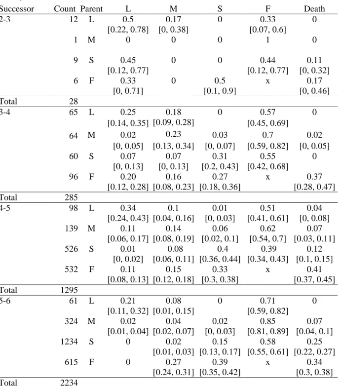
GU types were estimated annually, from the second to the sixth year of growth (Table 1). When long GUs were considered, no or few transitions toward short GU or meristem death took place in any year, while the most frequent transitions were toward another long or a floral GU. When medium GUs were considered, the most frequent successor in all years was a floral GU. A small number of medium GUs was followed by another medium GU, while an even small number was followed by a long GU. Direct transitions toward a short GU or death

were rare. When the parent GU was short, the most frequent transitions were toward another short or a floral GU, depending on the year. This change in transitions with years resulted

from the alternating flowering behaviour of Fuji cultivar (Costes et al. 2003). The transitions

from floral GU towards long GU decreased from the second to the fourth year of growth, while those toward medium GU increased. However, the most frequent transitions from floral GU were toward short GU or meristem death.

Similarly, axillary bud fates were explored during tree ontogeny, for different GU types

and years of growth, in order to estimate the parameters of HSMC (Renton et al. 2006). In

previous studies, the branching pattern along one-year-old trunks were shown to be organised in successive zones, and hidden semi-Markov chains were proposed to model this structure (Costes and Guédon 2002). This approach was further extended to explore how branching patterns, described at metamer scale along GUs, change during tree ontogeny. From the initial database, all GUs of the two Fuji trees were extracted and classified by type, year of growth and branching order. For each GU, the axillary bud fates were observed metamer by metamer and represented as a sequence of symbols corresponding to five types of lateral growth (latent

bud, and short, medium, long, and floral lateral GUs). First, all these sequences were used to

estimate a single HSMC composed of six successive transient states followed by an “end”

state (Fig. 1; see Renton et al. (2006) for details on model building). Second, each observed

sequence was optimally segmented in branching zones, using the estimated HSMC. Bivariate sequences were built by associating each observed sequence with the corresponding optimal segmentation in branching zones. The resulting bivariate sequences were grouped hierarchically according to the GU length, year of growth, and branching order. Parameters were estimated for each group of bivariate sequences on the basis of counts for the transition between successive branching zones, the branching zone length and the branching type composition of branching zones. The comparison of model parameters between these groups

highlighted similarities between GUs: the composition and relative position of the latent bud, floral and short-lateral zones were invariant within the GUs. The probability of occurrence of the floral zone changed with years, showing the alternative fruiting behaviour of ‘Fuji’ cultivar. Moreover, during ontogeny, branching patterns tended to become simplified due to the disappearance of the central zones and a progressive reduction of the floral zone length

with GU length (Renton et al. 2006). To formalize these results in MAppleT, a single subset

of parameters was used to represent mixtures of possible axillary GUs in branching zones and occupancy distributions for zones that were the same for all GU types and years, while different subsets of parameters were used depending on the type of parent GU and the year of growth for transition probabilities between branching zones and occupancy distributions for zones that differed between GU types or years.

In HSMC, the length of the sequences is a property of the model if an artificial “end” state is added to the model, and does not depend on the branch location. This may lead to unrealistic sequence length, ignoring the experimentally found decrease in the number of

metamers per GU with tree age (Costes et al. 1997 and 2003). We thus extracted from the

initial database the empirical distribution of number of metamers per GU (Fig 2). On the basis of this distribution, we selected limits for the range of sequence lengths according to the GU type and year of growth. The sequences generated by HSMC were then accepted or rejected depending on the correspondence between their length and the range of possible lengths for each GU type and year of growth.

Chronological control of morphogenesis and organ dimensions

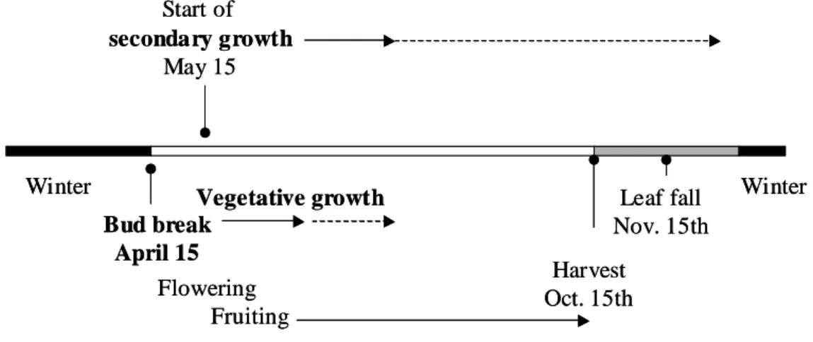
In MAppleT, a calendar defines the starting dates of simulated processes, i.e. primary and secondary growth (Fig. 3). However, individual organs at the metamer scale develop according to their own chronology, as they appear during the whole season. In each GU

category, new metamers are produced with a plastochron of three days. This value corresponds to the mean observed over a growing season for two different apple tree cultivars, ‘Starkrimson’ and ‘Rome Beauty’, grown with two different rootstocks (Costes and Lauri 1995). The period over which a metamer elongates was set to ten days according to observations of J.J. Kelner (personal communication). Measurements carried out on Fuji cultivar (unpublished data), showed that the final length of internodes depended on the internode position in the shoot, such that the internodes at the beginning and end of each GU were shorter than those in the middle. In MAppleT, this variation was modelled by attributing different lengths to internodes according to the branching zone along the shoot to which they belong.

Following field observations of Fuji leaf development collected by Massonnet (2004), it was assumed in MAppleT that leaves grow sigmoïdally over twelve days, at which time they reach maturity. Similarly, according to field observations of flowering and harvest dates in Fuji (J.L. Regnard, personal communication), we assumed that, if a metamer supports an inflorescence, the flowers last for ten days and, if it becomes a fruit, the fruit lasts until harvest (approximately 150 days). We also assumed that each inflorescence develops into one

fruit at most, which corresponds to the usual thinning practices (Costes et al. 2006). An

expolinear model, i.e. an exponential function followed by a linear function, had been

proposed by Lakso et al. (1995) to estimate the increase in mass of a fruit over time, and was

calibrated to the fruit of Fuji during a previous study (Massonnet 2004). This expolinear model with parameters for Fuji was used in MAppleT.

As large and rapid bending of axes is usually observed in fruit trees over a fruiting season, the intra-year dynamics of diameter growth must be taken into account in biomechanical

computations (Alméras et al. 2004). In MAppleT, the widths of the internodes were

used the metaphor introduced by these authors that considers each distal end of a plant as an origin of a vascular strand (a “pipe”), and that at each branching point, these strands are bundled together to form a larger, composite strand. According to this metaphor and a formulation proposed by Murray (1927) and further analyzed by MacDonald (1983), the

radius, r, of an internode is determined by the formula P

b P a

P _{r r}

r = +

,

lateral internode borne on the current internode, rb to the internode following the current

internode along the axis, and P is a fixed parameter, which we call the pipe model exponent. However, Suzuki and Hiura (2000) showed that this model explains allometry relationship at the level of the whole tree, but does not always apply to the current shoot. In particular, the pipe model formulation implies that growth in diameter occurs only when new internodes are added. To verify this assumption, we used a previously collected dataset of one-year-old floral GUs of Golden Delicious cultivar (Benzing 1999). This dataset characterized both the within-year dynamics of primary growth, i.e. number of new metamers, and growth in diameter (Fig. 4). Observations showed that primary growth of the shoots was found to start in mid-April and stop at the beginning of June. On the other hand, the diameter at the shoot base increased over the growing season in two distinct periods: rapidly from bud burst to the end of May and more slowly from mid-June to the end of the growing season. This demonstrated that growth in diameter continues even after the cessation of primary growth. Moreover, in a previous study carried out on apricot tree, the basal diameter of one-year-old shoots was found to be linearly related to the number of internodes, independently of the fruit load (Costes et al. 2000). Following these experimental data, we modelled the secondary growth in MAppleT by augmenting the diameter of the terminal internode continuously after the cessation of primary growth. This was done using the formula

2 3 4 5 6 7 − − − + = min max min min , max , min , ) ( ) ( ) ( n n n s n r r r s ra a a a ,

where ra(s) is the radius of the terminal internode of shoot s at the end the growing season,

min , a

r is the initial radius of this internode upon its creation (set to 0.75mm, Table 2), ra,maxis

the maximum radius observed at the end of the growing season for any terminal internode

(ra,maxwas set to 6mm according to field observations), n(s) is the number of internodes of

shoot s at the end of primary growth, and nminand nmaxare the minimum and maximum

numbers of metamers observed in the population of shoots of the same type as s. ra(s) is thus

located between ra,minand ra,maxproportionally to the status of shoot s in the population, as

defined by its number of metamers.

Determination of plant geometry using biomechanics

In MAppleT, the shape of each branch is calculated according to the biomechanical component of the model. Our method simulates branch bending and twisting, and the resulting permanent changes of branch shape (“shape memory”), following Fournier's treatment of woody stems as elastic beams (rods) subject to primary and secondary growth (Fournier 1989, Fournier et al. 1991a and 1991b). L-system implementations of Fournier’s model were originally developed by Jirasek et al. (2000) and Taylor-Hell (2005); a tutorial introduction to biomechanical modelling using L-systems is also presented by Prusinkiewicz

et al. (2007)3. The use of L-systems does not introduce new elements to the mechanics of

Fournier’s model, but facilitates the organization of computation by seamlessly updating the system of equations that need to be solved when new metamers are added, and by integrating all aspects of MAppleT within a single software environment. The biomechanical component

3

Mathematically, the equations used in our approach represent a finite-difference discretization of the underlying partial differential equations (Jirasek et al. 2000), which capture the mechanics of elastic rods (Landau and Lifshitz 1986). We have chosen finite differencing over finite element methods, because finite differencing is fully applicable to linear and branching structures, and is simpler to implement.

of MAppleT incorporates changes in shape due to the formation and impact of reaction wood, changes in the mechanical properties of wood with time, and the loading and unloading of fruits. The bending model is derived from the work of Taylor-Hell (2005), while changes in shape due to reaction wood and loading/unloading are derived from the work of Alméras (2001), and Alméras et al. (2002 and 2004).

In the biomechanical model, each point of a shoot axis is associated with a moving

U L H 2 2 2

frame, three orthogonal unit-length vectors that indicate the heading, upwards and left directions (Prusinkiewicz and Lindenmayer 1990, Prusinkiewicz et al. 2001). Bending and twisting correspond to rotations of this frame. The rate of rotation is expressed as

dl d dl d dl dθH_, θL_, θU =

Ω , where the individual derivatives represent the rates of rotation around

the H L U

2 2 2

,

, vectors, and l is a position along the shoot axis. For computational purposes, we

assumed that each shoot axis is discretized into a sequence of rigid internodes connected at flexible nodes (joints) (Fig. 5). The mass of each internode is assumed to be concentrated at its distal node.

The shape of the axis depends on the torques acting on its nodes. When calculating these torques, two factors are initially taken into account: the force of gravity and a combined effect of photo- and gravitropism, which is abstracted as an orthotropic force. The gravity

component of the torque

τ

2

that acts on the proximal node of an isolated internode i is

equal to ig

l

H

m

g

2

2

2

×

=

τ

2

is its heading vector,

mi is the mass of the distal node,and g

2

is the gravity acceleration. This equation is recursively

extended to an entire axis using the formula i i i ig

g i

l

H

M

g

τ

τ

2

=

2

×

2

+

2

1

(Prusinkiewicz et al. 2007). A further extension to branching structures is accomplished by adding torques from all branches originating at the same node (Fig. 5c).

The combined effect of phototropism and negative gravitropism is simulated by turning shoots upward (Hangarter 1997). Although phototropism may act on both elongating and non-elongating shoots (Matsuzaki et al. 2007), we only consider the non-elongating (leafy) internodes.

Specifically, we assume that leafy nodes are subject of a torque it liHi T

2 2

2

τ

of a leafy shoot is thus

τ

τ

τ

2

2

2

+

=

To calculate the resulting change in frame orientation, we decompose torque

τ

2

components

τ

τ

τ

2 2 2

,

, axes at node i, find the corresponding

rotations , iH iH r iH R

τ

τ

τ

Ω around these axes, and compose them into

the combined rotation r

i

Ω (Jirasek et al. 2000). Assuming that the rotations Ωr_iH,Ωr_iLand Ω_iUr

are small, their composition does not significantly depend on the order of rotations, and thus is well defined (Goldstein 1980).

In the above formulas, R_iH is the torsional rigidity of the axis at node i, while R_iL and

iU

R are flexural rigidities in the direction of L

2

and U

2

axes, assumed to coincide with the principal axes of the cross-section of the axis at node i. This assumption is automatically satisfied if the branches have circular cross-section and the distribution of material properties

in the branches is radially symmetric, which we assume in the model4. In principle, the

flexural rigidity is calculated using the formula R_iL =R_iH =EI where E is the Young’s

modulus of the material, and I is the second moment of the area of the branch cross-section,

4

equal to 4

4r

π

for an axis passing through the centre of the circle of radius r (Niklas 1992).

The torsional rigidity is calculated using an analogous formula, R_iH =GJ , where G is the

shear modulus of the material, and J is a torsional constant, equal to 4

2r

π

for a circle of radius

r (Niklas 1992). In MAppleT, these formulas are modified to take into account the reaction

wood, as described below.

The bending of branches due to the combination of gravity and tropism, initially of elastic nature, leads to a permanent change of branch shape resulting from the memory effect of secondary growth, as discussed by Fournier et al. (1991a and 1991b) and Jirasek et al. (2000)

The rotation Ω_iat node i is thus a linear combination of two terms: rotation r

i

Ω due to the

current torque acting on this node, and rotation m

i

Ω due to the shape memory.

In MAppleT, we also assumed that some amount of reaction wood is produced each year in an angular section of the outer wood layer (Wilson and Archer 1977, Fig. 6a). The proportion of reaction wood in this layer is calculated using an empirical relation that was

estimated in Alméras’s studies (Alméras 2001): Pr=0.164−0.178∆

θ

proportion of reaction wood in the outermost cambial layer and ∆θ is the change in shoot

inclination in radians (i.e. the change in H

2

at each time step, which is negative when the branch bends). The way this formula is used in MappleT relies on the assumption that the reaction wood does not play a major role in shape regulation in fruit trees, as previously demonstrated by Alméras et al. (2004) on different apricot cultivars. Here, the reaction wood is assumed to only prevent large bending movements and, contrary to observations on several

forest tree species, does not have any active up-righting function. Moreover, according to

these previous observations on apricot tree, the amount of reaction wood also depends on the shoot orientation with respect to gravity, since an upright shoot develops less reaction wood

to make the amount of reaction vary with shoot orientation. The relationship used is:

θ

, where g2' is a unit vector in the direction opposite to

gravity. To keep the calculations simple, when reaction wood is present, it was assumed that the second moment of area of the initial cross-sectional area is augmented with an additional contribution for each annular radial section of reaction wood (Fig. 6b). The contribution of the radial section of reaction wood to the section rigidity was assumed proportional to moment of

area calculated as follows: ( ' )( sin )

8

1 4− 4

γ

γ

= r r

Is where γ is the angular section of reaction

wood (γ = 2π Pr, in radians) in the cambial layer, r and r’ are the inner and outer radius

respectively (Fig. 6b). The total second moment of area of an internode was thus expressed as

1 = + = n k sk I c I I 1 ,

α

radial section of cambial layer k and α is a coefficient that controls the reaction wood effect.

The biomechanical model was implemented in terms of information flow through the plant

structure (Jirasek et al., 2000, Taylor-Hell 2005, Prusinkiewicz et al. 2007). The simulation is

carried out be iterating two computational phases. First, bending and twisting moments are calculated in a backward scan of the L-system string (information is passed basipetally). In

this phase, the torques

τ

2

that apply to all internodes i are computed iteratively from the

distal to the proximal end of the branch, given its current configuration. Second, the shape of the branch is updated in a forward (acropetal) scan of the string, taking bending moments and

the resulting angles between the internodes into account. The consecutive node positions Ii

2

are then calculated using the formula I_i I_i l_iH_i

2 2 2

+ =

+1 . This procedure is iterated until the

position of the branch nodes converges toward a stable solution.

Due to the stochastic nature of Markov models, different seeds used to initialize MappleT’s random number generator result in different topologies of simulated trees. These differences propagate to the level of tree geometries, which vary even if the parameter values of the biomechanical model are the same (Fig. 7). Furthermore, MappleT generates not only the structure and form of trees at a particular developmental stage, but entire developmental sequences. Each sequence can be visualized as a series of images representing different stages of tree development (Fig. 8) or as an animation of development. We observed that trees generated by MappleT had a visually similar character to a Fuji tree that was digitized and

visualised with with PlantGL viewer (Pradal et al., 2007), at the same development stage

(here six-year-old trees).

To compare simulated and observed trees quantitatively, the architecture of trees generated with L-studio were represented, at the end of each year, as Multi-scale Tree Graph (MTG; Godin and Caraglio 1998), containing both the topological and geometrical information of each plant entity. A number of descriptors was extracted, at different scales of observation and then compared between simulated and digitised trees (two digitised Fuji trees were available in the database, see Materials and Methods). For these comparisons, our strategy was to use coarser scales than those at which the model was formulated originally. We then analyzed whether the properties that were not specified explicitly in the model would emerge from the system integration.

Regarding tree topology, the main assumption in Markovian models concerned local dependencies between GUs with transition probabilities according to their type and year of growth, and between successive branching zones at the metamer scale. In contrast, no assumption was made regarding the total number of growth units of a given type at the entire tree scale. The corresponding counts thus represent a property of the simulated trees that emerged from the aggregation of the four-state Markov chain and the HSMCs models for

branching. These counts cannot be directly calculated from the elementary models and were rather extracted from both simulated and observed trees over six successive years. Comparisons of GUs, made separately for terminal and lateral positions, showed that simulation results were most of the time close to field data (Fig. 9). The main pattern related to tree ontogeny, the decrease in the number of long GUs, first in lateral and one year later in terminal positions, was correctly simulated. Similarly, the transition from the majority of floral GUs in lateral positions in the third and fourth years of growth to the majority of floral GUs in terminal positions in the subsequent years was adequately simulated by the model. This change in the floral GU position can be interpreted as a consequence of the decrease in the number of long GUs and the considerable increase in the number of short GUs in the fifth and sixth years.

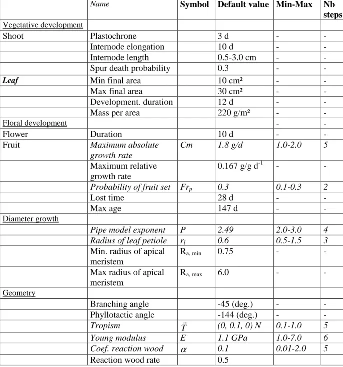
Regarding geometry, the global shape of the simulated trees emerged from the combination of each particular simulated topology with the biomechanical model. This global shape could not be predicted, as it results from the aggregation of a large number variables, and their integration throughout time. To quantify comparisons, a number of descriptors of shoot geometry, such as the basal diameter, length, inclination or curvature were calculated for both simulated and observed trees. In order to perform a preliminary sensitivity analysis, these descriptors were obtained for different values of seven main parameters of the model (see Table 2). Comparisons were made for branches 20 cm in length or more. Both length and basal diameters were under-estimated at orders 1 and 2, for all the values of the pipe model exponent and the radius of the leaf petiole. More correct values were obtained at higher orders

using the default value P = 2.5 (data not shown and Fig. 10a). This suggests that other

variables such as internode lengths and distal diameters must be further investigated. In particular, the model sensitivity to the variation of apex radius at the beginning of each growing season should be considered. Regarding branch geometry, our analysis mainly

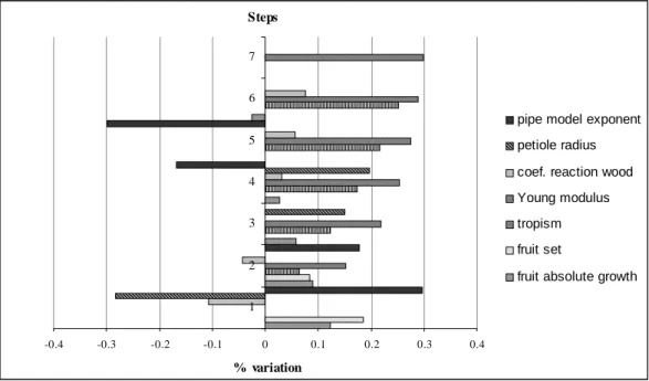
focuses on the branch chord inclination (Fig. 10b and Fig. 11). The independent variation of the seven parameters over 3 to 7 steps (see Table 2) induced a variation of branch chord inclination that ranged from 2 to 30% with respect to that obtained using default values of all parameters (Fig. 11). The parameters that induced the largest variations in branch inclination were the pipe model exponent, petiole radius and Young modulus. In contrast, the parameters related to fruits (fruit set probability and fruit absolute growth rate) had the lowest impact on

branch chord inclination. Moreover, we examined the impact of the pipe model exponent P on

branch chord inclination for different branch orders (Fig. 10b). As was the case for the branch basal diameter, the mean branch chord inclination was under-estimated for branches of order 1 while it was quite correct for higher orders. At coarser scales, convex hulls that included the fruiting branches and the distal part of the trees were calculated with PlantGL viewer (Fig. 12). The mean value of these hull surfaces compared between simulated and observed trees were in the same range than those obtained when the default value of the pipe model exponent was used in the simulations (data not shown).

Discussion and conclusion

Mixing stochastic and mechanistic model components, MAppleT is a useful tool for simulating the development of apple trees as affected by gravity. A distinctive characteristic of MAppleT is the close connection between the field data and simulations. This connection made it possible to integrate previously existing, but scattered data, and to estimate the model parameters on the basis of observations.

To model tree topology, we used a two-scale stochastic process inspired by previous work

(Fine et al. 1998). Although only two trees were analysed and the first year of growth were

insufficiently characterized, the large number of GUs and transitions between their types allowed us to estimate the model parameters accurately from the second third to the sixth year

of growth, as demonstrated by the confidence intervals in Table 1. Interestingly, a related approach has been previously used to simulate plant architectures for computer graphics purposes, but did not take into account the biological background and field data on the

modelled plants (Wang et al. 2006).

In MAppleT, an efficient strategy was proposed to keep the overall Markovian model

parsimonious, based on the study carried out by Renton et al. (2006). This strategy relies on

the analysis of similarities and discrepancies between branching structures during tree ontogeny. Some parameters (observation distributions) were found to be similar between HSMCs for long and medium GUs while others (transition probabilities and occupancy distribution) depended on the GU type and year of growth. Since the succession of states is almost deterministic in the case of apple tree (Fig. 1), the underlying “left-right” semi-Markov

chain is degenerated: for each state i, (except the “end” state), q_ii+1 =1 and q_ij =0 for

1

+ ≠i

j . Hence, there are very few independent transition probabilities. Moreover, the

branching zone modelled by state 2 in the HSMC shown in Fig. 1 only occurs in the two first

years of growth (Renton et al. 2006). Thus this state 2 is systematically skipped, except for

long GUs in the first two years. This leads to another decrease in the number of parameters. Branching sequences generated by the HSMCs for long and medium GUs are filtered (either accepted or rejected) according to a length criterion. We are aware that this strategy is not optimal and is likely to introduce a bias into the branching sequences. In future work, we intend to improve this estimation strategy in order to obtain a family of HSMCs that realizes a better compromise between the fit to the data and the parsimony of the overall family of HSMCs. Sophisticated parameterizations could be proposed, including (i) tied parameters between HSMCs, (ii) covariates that influence specific parameters (e.g. year of growth influencing transition distributions).

The model simulates the effect of gravity on the plant form, yielding simulated tree forms that are visually similar to the observed trees. However, the effect of gravity on morphogenesis (gravimorphism) is only partly introduced. The median location of long and medium lateral GUs along the parent GU that has been interpreted as a result from bending by

Renton et al. (2006), is taken into account in MAppleT through the HSMC models for

branching. In further developments of the model, the purely stochastic description of branching should be augmented by a causal feedback between shoot bending and lateral development.

As mentioned above, the present study is closely linked to a number of field observations. In the case of tree 3D geometry, available databases allowed us to perform extensive comparisons between simulated and observed trees. These comparisons revealed some discrepancies between observations and the model outputs. For instance, branch inclination for some orders is not simulated correctly (Fig. 8). This may be related to our use of a constant value for the pipe model exponent, independent of the shoot type and branching order. One approach to improve our results may be based on a refinement of the pipe model,

as proposed by Deckmyn et al. (2006) or on the introduction of a carbon allocation model

such as that used in L-Peach (Lopez et al. this issue).

Although a large number of field observations was used in the present study, more precise estimated or direct measurements might be necessary for some parameters, such as those used for calculating the radial portion of the outermost cambial layer that became reaction wood,

which presently come from Alméras’ study on apricot tree (Alméras et al. 2002).

Furthermore, the model is stochastic in nature which makes it necessary to use a statistical methodology for its validation. It is noticeable that a methodology to perform the model validation on objective bases is currently missing for Functional-Structural Plant Model (FSPM) validation. Despite these limitations, MAppleT is one of the fist attempt to simulate a

fruit tree that develop over years with a global shape reacting to gravity. With L-Peach (Allen

et al. 2005, Lopez et al. this issue), MAppleT contributes to the foundation of innovative tools

for fruit tree simulation. Considering that tree responses to gravity, via the induced changes in tree geometry, have an impact on light interception, within-tree micro-climate, and fruit production and quality, MAppleT will allow further investigations on horticultural practices, as recently initiated by Lopez et al. (this issue). Moreover, the genetic variation of shoot morphology that has been demonstrated in the apple tree (Segura et al., 2007) could also be simulated through virtual scenario. From a methodological point of view, the proposed modelling approach, which aggregates stochastic and mechanistic models, and the proposed first validation of the model outputs, that include tree topology and global shape changes in response to gravity, are likely to found applications in other plants as well.

Aknowledgements:

We thank Julia Taylor-Hell for kindly making her model of branch bending in poplar trees available. We also thank Fredéric Boudon for his assistance on the Geom module from PlantGL, Jean-Jacques Kelner and Jean-Luc Regnard for allowing us to use their observations of apple trees. This research was supported in part by the Natural Sciences and Engineering Research Council of Canada Discovery Grant RGPIN 130084-2008 to P.P. The postdoctoral positions of C. Smith and M. Renton were granted by the INRA Department of Genetics and Plant Breeding.

Bibliography

Adam B, Sinoquet H and Godin C (1999) 3A version 1.0: Un logiciel pour l'Acquisition de

AMAPmod et de la géométrie par digitalisation 3D. Guide de l'utilisateur. INRA-PIAF Clermont-Ferrand (France).

Allen M, Prusinkiewicz P, Dejong T (2005) Using L-systems for Modeling Source-Sink

Interactions, Architecture and Physiology of Growing Trees: the L-PEACH Model. New

Phytologist 166, 869–880.

Alméras T (2001) Acquisition de la forme des axes ligneux d'un an chez trois variétés d'abricotier: confrontation de données expérimentales à un modèle biomécanique, PhD. Thesis, Montpellier SupAgro.

Alméras T, Gril J, Costes E (2002) Bending of apricot-tree branches under the weight of

axillary productions: confrontation of a mechanical model to experimental data. Trees 16,

5-15.

Alméras T, Costes E, Salles JC (2004) Identification of biomechanical factors involved in

stem form variability between apricot tree varieties. Annals of Botany 93: 455-68.1

Ancelin, P, Fourcaud T, Lac P (2004) Modelling the Biomechanical Behaviour of Growing Trees at the Forest Stand Scale. Part I: Development of an Incremental Transfer Matrix

Method and Application to Simplified Tree Structures. Annals of Forest Science 61, 263–

275.

Benzing S. (1999) Patterns of vegetative and reproductive growth in apple (Malus x

domestica Borkh.). Master thesis, Fac. de Wiesbaden / Geisenheim.

Costes E, Lauri PÉ (1995) Processus de croissance en relation avec la ramification sylleptique

et la floraison chez le pommier. In ‘Architecture des arbres fruitiers et forestiers’. (Ed. J Bouchon) pp 41-50. (INRA Editions, Paris).

Costes E, Guédon Y (2002) Modelling branching patterns on 1-year-old trunks of six apple

Costes E, Lauri PE, Lespinasse JM. (1995) Modélisation de la croissance et de la ramification chez quelques cultivars de Pommier. In ‘Architecture des arbres fruitiers et forestiers’. (Ed. J Bouchon) pp 27-39. (INRA Editions, Paris).

Costes E, Fournier D, Salles JC (2000) Changes in primary and secondary growth as

influenced by crop load effects in 'Fantasme®' apricot trees. The Journal of Horticultural

Science & Biotechnology 75, 510-529.

Costes E, Lauri PE, Régnard JL (2006) Tree Architecture and Production. Horticultural

Reviews 32, 1-60.

Costes E, Sinoquet H, Kelner JJ, Godin C (2003) Exploring within-tree architectural

development of two apple tree cultivars over 6 years. Annals of Botany 91, 91-104.

Crabbé J, Escobedo-Alvarez JA (1991) Activités méristématiques et cadre temporel assurant la transformation florale des bourgeons chez le Pommier (Malus x Domestica Borkh., cv.

Golden Delicious). L'Arbre: Biologie et Developpement: Naturalia Monspeliensia Special

n°, 369-79.

Deckmyn G, Evans SP, Randle TJ (2006) Refined pipe theory for mechanistic modeling of

wood development. Tree Physiology 26, 703-717.

Durand J-B, Guédon Y, Caraglio Y, Costes E (2005) Analysis of the plant architecture via

tree-structured statistical models: The hidden Markov tree models. New Phytologist 166,

813-825.

Fine S, Singer Y, Tishby N (1998) The hierarchical hidden Markov model: Analysis and

applications. Machine Learning 32, 41-62.

Fournier M (1989) Mécanique de l’arbre sur pied: maturation, poids propre, contraintes climatiques dans la tige standard. PhD thesis, INP de Lorraine.

Fournier M, Chanson B, Guitard D, Thibaut B (1991a) Mechanics of standing trees: modelling a growing structure submitted to continuous and fluctuating loads. 1. Analysis

of support stresses. Annals of Forest Science 48, 513-525.

Fournier M, Chanson B, Guitard D, Thibaut B (1991b). Mechanics of standing trees: modelling a growing structure submitted to continuous and fluctuating loads. 2.

Tridimensional analysis of maturation stresses. Annals of Forest Science 48, 527-46.

Gautier H, Mech R, Prusinkiewicz P, Varlet-Grancher C (2000). 3D Architectural Modelling of Aerial Photomorphogenesis in White Clover (Trifolium repens L.) using L-systems.

Annals of Botany 85, 359-370.

Godin C (2000). Representing and encoding plant architecture: a review. Annals of Forest

Science 57, 413-438.

Godin C, Caraglio Y (1998) A multiscale model of plant topological structures. Journal of

Theoretical Biology 191, 1-46.

Godin C, Costes E, Sinoquet H (1999). A method for describing plant architecture which

integrates topology and geometry. Annals of Botany 84, 343-357.

Goldstein H (1980) Classical mechanics. Second edition. Reading: Addison-Wesley.

Guédon Y (2003) Estimating hidden semi-Markov chains from discrete sequences. Journal of

Computational and Graphical Statistics 12, 604-639.

Guédon Y, Barthélémy D, Caraglio Y, Costes E (2001) Pattern analysis in branching and

axillary flowering sequences. Journal of Theoretical Biology 212, 481-520.

Hanan J, Room P (1997) Practical aspects of virtual plant research. In ‘Plants to ecosystems’. (Ed. Michalewicz MT) pp 28-45. (Collingwood: CSIRO Publishing).

Hanan J, Hearn AB (2002) Linking physiological and architectural models of cotton.

Agricultural systems 14, 1-31.

Jirasek, C., Prusinkiewicz, P. and Moulia B (2000) Integrating Biomechanics into Developmental Plant Models Expressed using L-systems. In ‘Plant biomechanics 2000’. (Eds HC Spatz and T Speck) pp 615–624. (Freiburg-Badenweiler, Georg Thieme Verlag). Karwowski R, Prusinkiewicz P (2003) Design and implementation of the L+C modeling

language. Electronic Notes in Theoretical Computer Science 86(2), 134-152.

Kelner JJ (2000) AIP AGRAF: Pour l’élaboration de la composition et l’aptitude à l’utilisation des grains et des fruits. (INRA, Paris).

Lakso AN, Grappadelli LC, Barnard J, Goffinet MC (1995) An expolinear model of the

growth pattern of the apple fruit. Journal of Horticultural Science 70, 389-394.

Lauri PÉ (2002) From tree architecture to tree training - An overview of recent concepts

developed in apple in France. Journal of the Korean Society for Horticultural Science 43,

782-8.

Lauri PÉ, Térouanne E, Lespinasse JM (1997) Relationship between the early development of apple fruiting branches and the regularity of bearing - An approach to the strategies of

various cultivars. Journal of Horticultural Science 72, 519-30.

Lindenmayer A (1968). Mathematical models for cellular interaction in development, Part I

and II. Journal of theoretical biology 18, 280-315.

Lopez G, Favreau RR, Smith C, Costes E, Prusinkiewicz P, DeJong PM (2008) Integrating simulation of architectural development and source-sink behaviour of peach trees by incorporating Markov chains and physiological organ function sub-models into L-PEACH. This issue.

MacDonald, N (1983) Trees and networks in biological models (Chichester: J. Wiley & Sons).

Massonnet C (2004) Variabilité architecturale et fonctionnelle du système aérien chez le

pommier (Malus x Domestica Borkh.) : comparaison de quatre cultivars par une approche

de modélisation structure-fonction. PhD Thesis, Montpellier SupAgro.

Matsuzaki J, Masumori M, Takeshi T (2007) Phototropic bending of non-elongating and radially growing stems results from asymmetrical xylem formation. Plant Cell and

Environment 30, 646-653.

Mech R, Prusinkiewicz P (1996) Visual models of plants interacting with their environment. Proceedings of SIGGRAPH, 397-410.

Murray C (1927) A relationship between circumference and weight in trees and its bearing on

branching angles. The Journal of General Physiology 10, 725-729.

Niklas K (1992) Plant biomechanics. An engineering approach to plant form and function. (Chicago: The University of Chicago Press).

C. Pradal, F. Boudon, C. Nouguier, J. Chopard, C. Godin 2007. PlantGL : a Python-based geometric library for 3D plant modelling at different scales. INRIA Research Report n°

6367, Nov. 2007, <http://www-sop.inria.fr/virtualplants/Publications/2007/PBNCG07/>.

Prusinkiewicz P (1998) Modeling of spatial structure and development of plants. Scientia

Horticulturae 74, 113-149.

Prusinkiewicz P, Lindenmayer A (1990) The algorithmic beauty of plants (New York: Springer Verlag).

Prusinkiewicz P, Mündermann L, Karwowski R, Lane B (2001) The use of positional information in the modeling of plants. Proceedings of SIGGRAPH 2001, pp. 289-300. Prusinkiewicz P, Karwowski R, Lane B (2007) The L+C plant-modelling language. In

‘Functional-structural plant modeling in crop production’. (Eds. J Vos, LFM. de Visser, PC. Struick, JB Evers) pp. 27-42. (Springer: The Netherlands).

Renton M, Kaitaniemi P, Hanan J (2005a). Functional-structural plant modelling using a combination of architectural analysis, L-systems and a canonical model of function.

Ecological Modelling 184, 277-298.

Renton M, Hanan J, Burrage K (2005b). Using the canonical modelling approach to simplify

the simulation of function in functional-structural plant models. New Phytologist 166,

845-857.

Renton M, Guédon Y, Godin C, Costes E (2006) Similarities and gradients in growth unit branching patterns during tree ontogeny based on a stochastic approach in ‘Fuji’ Apple

Trees. Journal of Experimental Botany 57, 3131–3143.

Segura V, Denancé C, Durel CE, Costes E (2007) Wide range QTL analysis for complex architectural traits in a 1-year-old apple progeny. Genome 50: 159-171.

Sinoquet H, Rivet P, Godin C (1997) Assessment of the three-dimensional architecture of

walnut trees using digitising. Silva Fennica 31, 265-73.

Shinozaki K, Yoda K, Hozumi K, Tira T (1964) A quantitative analysis of plant form – the

pipe model theory. (i) basic analyses. Japanese Journal of ecology 14, 97-105.

Suzuki M, Hiura T (2000) Allometric differences between current-year shoots and large

branches of deciduous broad-leaved tree species. Tree Physiology 20, 203-209.

Taylor-Hell J (2005) Biomechanics in botanical trees. Master thesis, University of Calgary. Thornby D, Renton M, Hanan J (2003) Using computational plant science tools to investigate

morphological aspects of compensatory growth. Computational Science - Iccs 2003, Pt Iv,

Proceedings, 708-717.

Wang R, Hua W, Dong Z, Peng Q, Bao H (2006) Synthesizing trees by plantons. Visual

Comput 22, 238-248.

White J (1979) The plant as a metapopulation. Annual Review of Ecological Systems 10,

Wilson BF and Archer RR (1977) Reaction wood: induction and mechanical action. Annual

Table 1. Transition probabilities between successive growth units (GUs), with associated counts and 95% confidence intervals, depending on the year of growth for two apple trees, cultivar ‘Fuji’. Four types of GU were considered: long GU (L), medium GU (M), short GU (S) and floral GU (F). Successor GU after a floral GU arose from sympodial branching.

Years, Parent- Successor

Successor Count Parent L M S F Death

2-3 12 L 0.5 0.17 0 0.33 0 [0.22, 0.78] [0, 0.38] [0.07, 0.6] 1 M 0 0 0 1 0 9 S 0.45 0 0 0.44 0.11 [0.12, 0.77] [0.12, 0.77] [0, 0.32] 6 F 0.33 0 0.5 x 0.17 [0, 0.71] [0.1, 0.9] [0, 0.46] Total 28 3-4 65 L 0.25 0.18 0 0.57 0 [0.14, 0.35] [0.09, 0.28] [0.45, 0.69] 64 M 0.02 0.23 0.03 0.7 0.02 [0, 0.05] [0.13, 0.34] [0, 0.07] [0.59, 0.82] [0, 0.05] 60 S 0.07 0.07 0.31 0.55 0 [0, 0.13] [0, 0.13] [0.2, 0.43] [0.42, 0.68] 96 F 0.20 0.16 0.27 x 0.37 [0.12, 0.28] [0.08, 0.23] [0.18, 0.36] [0.28, 0.47] Total 285 4-5 98 L 0.34 0.1 0.01 0.51 0.04 [0.24, 0.43] [0.04, 0.16] [0, 0.03] [0.41, 0.61] [0, 0.08] 139 M 0.11 0.14 0.06 0.62 0.07 [0.06, 0.17] [0.08, 0.19] [0.02, 0.1] [0.54, 0.7] [0.03, 0.11] 526 S 0.01 0.08 0.4 0.39 0.12 [0, 0.02] [0.06, 0.11] [0.36, 0.44] [0.34, 0.43] [0.1, 0.15] 532 F 0.11 0.15 0.33 x 0.41 [0.08, 0.13] [0.12, 0.18] [0.3, 0.38] [0.37, 0.45] Total 1295 5-6 61 L 0.21 0.08 0 0.71 0 [0.11, 0.32] [0.01, 0.15] [0.59, 0.82] 324 M 0.02 0.04 0.02 0.85 0.07 [0.01, 0.04] [0.02, 0.07] [0, 0.03] [0.81, 0.89] [0.04, 0.1] 1234 S 0 0.02 0.15 0.58 0.25 [0.01, 0.03] [0.13, 0.17] [0.55, 0.61] [0.22, 0.27] 615 F 0 0.27 0.39 x 0.34 [0.24, 0.31] [0.35, 0.42] [0.3, 0.38] Total 2234

Table 2. List of parameters used in MAppleT, with those used in the sensitivity analysis indicated in italics. Default values are indicated for each parameter. The range of variation and the number of steps tested in the sensitivity analysis is indicated only for the parameters used. This table does not include Markovian model parameters.

Name Symbol Default value Min-Max Nb

steps

Vegetative development

Shoot Plastochrone 3 d - -

Internode elongation 10 d - -

Internode length 0.5-3.0 cm - -

Spur death probability 0.3 - -

Leaf Min final area 10 cm² - -

Max final area 30 cm² - -

Development. duration 12 d - -

Mass per area 220 g/m² - -

Floral development - -

Flower Duration 10 d - -

Fruit Maximum absolute

growth rate

Cm 1.8 g/d 1.0-2.0 5

Maximum relative growth rate

0.167 g/g d-1 - -

Probability of fruit set Frp 0.3 0.1-0.3 2

Lost time 28 d - -

Max age 147 d - -

Diameter growth

Pipe model exponent P 2.49 2.0-3.0 4 Radius of leaf petiole rl 0.6 0.5-1.5 3

Min. radius of apical meristem

Ra, min 0.75 - -

Max radius of apical meristem

Ra, max 6.0 - -

Geometry

Branching angle -45 (deg.) - -

Phyllotactic angle -144 (deg.) - -

Tropism _T2 (0, 0.1, 0) N 0.1-1.0 5 Young modulus E 1.1 GPa 1.0-7.0 6 Coef. reaction wood

α

Figure Captions

Fig 1. Hierarchical stochastic model representing tree topology. Successions and branching between entities are represented by ‘<’ and ‘+’ respectively. At the growth unit (GU) scale, the succession of GUs along an axis is modelled by a 4-state Markov chain. The four “macro-states” are long (L), medium (M), short (S) and flowering (F) GU. The long and medium macro-states activate HSMCs with between-scale transitions (doted arrows). The figure shows only the activation from a long GU macro-state. HSMCs model the GU branching structure at the metamer scale, as a succession of zones with specific composition of axillary GUs (for instance a mixture of long, medium and short axillary GUs is observed in state 2). The HSMC ends with an artificial final state which gives control back to the pending macro-state. Likewise, for each axillary position, between-scale transitions give the control back to the macro-state model corresponding to the type of axillary GU generated by the HSMC (the figure illustrates only these transitions from HSMC state 2).

Fig 2. Relationship between GU type and limits used in MAppleT to partition the sequence lengths (i.e. number of internodes per GU) into classes. Based on the distributions of number of internodes for medium and long GU (Fig. 1b,c), the limit between medium and long GU was fixed at 15 internodes (indicated with an arrow). Based on the distributions of number of internodes per year for long GU (Fig. 1c), the maximum possible length decreased with the year of growth.

Fig 3. Calendar of simulated events over a year in MAppleT. In this calendar, new metamers develop with a plastochrone of 3 days and each organ (i.e. leaves, internodes, flowers, and fruits) has its own chronology for development.