Geophysical Journal International
Geophys. J. Int. (2012)190, 457–462 doi: 10.1111/j.1365-246X.2012.05481.x
GJI
Seismology
Predictability of repeating earthquakes near Parkfield, California
J. Douglas Zechar
1,2and Robert M. Nadeau
31Swiss Seismological Service, ETH Zurich, Sonneggstrasse 5, NO H 3, 8092 Zurich, Switzerland. E-mail: jeremy.zechar@sed.ethz.ch 2Department of Earth Sciences, University of Southern California, 3651 Trousdale Pkwy, Los Angeles, CA 90089, USA
3Berkeley Seismological Laboratory, University of California, Berkeley, CA 94720, USA
Accepted 2012 March 27. Received 2012 February 13; in original form 2011 July 4
S U M M A R Y
We analyse sequences of repeating microearthquakes that were identified by applying wave-form coherency methods to data from the Parkfield High-Resolution Seismic Network. Be-cause by definition all events in a sequence have similar magnitudes and locations, the temporal behaviour of these sequences is naturally isolated, which, coupled with the high occurrence rates of small events, makes these data ideal for studying interevent time distributions. To characterize the temporal predictability of these sequences, we perform retrospective forecast experiments using hundreds of earthquakes. We apply three variants of a simple algorithm that produces sequence-specific, time-varying hazard functions, and we find that the sequences are predictable. We discuss limitations of these data and, more generally, challenges in identifying repeating events, and we outline the potential implications of our results for understanding the occurrence of large earthquakes.
Key words: Probabilistic forecasting; Probability distributions; Earthquake interaction,
forecasting, and prediction; Seismicity and tectonics; Statistical seismology.
1 I N T R O D U C T I O N
The study of earthquake interevent times is one of the oldest and most fundamental problems in seismology. Today, a common first-order approach to estimate the hazard that a particular fault poses is to compare the average recurrence interval with the time elapsed since the last large earthquake on the fault. If we consider an ideal-ized model of the earth in which tectonic loading and fault strength are relatively constant and stress is released only in earthquakes of a characteristic size, we might expect periodic or quasi-periodic earthquake sequences. Such a simple model was previously believed to describe the occurrence of earthquakes of about magnitude 6 at Parkfield, California. Indeed, this belief was the basis for an official earthquake prediction made by the US National Earthquake Pre-diction Evaluation Council (Shearer 1985; Jackson & Kagan 2006), and this belief also motivated the development of a multidisciplinary observatory at Parkfield, including the Parkfield High-Resolution Seismic Network (HRSN). The official Parkfield Earthquake pre-diction was indisputably wrong—no earthquake occurred within the specified space–time–magnitude window. Yet the observatory inspired by the prediction experiment made Parkfield one of the best-studied earthquake sources in the world, and it also aided the discovery of many small repeating earthquake sequences (Nadeau
et al. 1995; Nadeau & Johnson 1998).
Understanding the temporal behaviour of large earthquakes has obvious importance to society, as this is one of the crucial steps
in accurately assessing seismic hazard. More generally, studying the occurrence times of large earthquakes can improve our under-standing of the link between the accumulation of stress from plate tectonics and its release via seismicity. However, large earthquakes happen relatively rarely and therefore data are scarce. On the other hand, small earthquakes are plentiful, and there has been no rigorous demonstration that the scaled space–time–magnitude distribution of small earthquakes is different from that of large earthquakes; indeed, the exponential distribution of magnitudes and the scaling of average recurrence times seems to extend from large earthquakes to at least the smallest earthquakes that are reliably recorded (Chen
et al. 2007; Boettcher et al. 2009). And the Regional Earthquake
Likelihood Models experiment in California has provided evidence that a forecast of intermediate to large earthquakes based on the spatial distribution of small earthquakes has substantial predic-tive skill (Schorlemmer et al. 2010). Moreover, there is no obvious distinction between the source physics of small and large events, and many workers have conducted experiments in laboratory settings and proposed that the results might apply at the scale of tectonic earthquakes (e.g. Beeler 2004). Although it is not obvious how to transfer knowledge gained from studies of small earthquakes to ap-plications of large earthquake forecasting, analysing the temporal behaviour of small earthquakes is in and of itself important.
It has been suggested that earthquake physics should be stud-ied at multiple scales (Ben-Zion 2008); in parallel, earthquake pre-dictability should be studied at multiple scales. Of the recent surge in
earthquake forecast experiments, almost all cover large geographic regions, focus on intermediate and large earthquakes and emphasize spatial predictability (Jordan 2006; Zechar et al. 2010). To com-plement these ongoing efforts, we have conducted predictability experiments concerning repeating microearthquakes at Parkfield. A repeating earthquake sequence is a set of events that occur ef-fectively in the same hypocentral region and yield highly similar seismograms, implying that the events have similar source mecha-nisms and repeatedly rupture the same fault patch. Clearly, repeating earthquakes are in some qualitative sense predictable because they happen in the same place, and in early studies of the Parkfield mi-croearthquakes, the quasi-periodicity of these sequences was noted (e.g. Nadeau & Johnson 1998, fig. 4; Nadeau & McEvilly 1999, fig. 2). In this study, we use straightforward statistical approaches to establish the quantitative temporal predictability of the Parkfield microrepeater sequences.
2 D AT A
The waveforms used in this study were recorded by the HRSN between 1987 and 2010 April 10 (inclusive). The HRSN was in-stalled in 1986–1987 as part of the Parkfield Prediction Experiment (Bakun & Lindh 1985) to help construct a detailed picture of the dynamic process of fault-zone failure prior to an expected M6 earth-quake. Data from this local-scale borehole network are unique in their high-frequency content and sensitivity to very low amplitude seismic signals [e.g. microearthquakes (M< 0), ambient noise and non-volcanic tremor] that have substantially advanced our under-standing of fault-zone structure, evolution and process relative to the rupture zone of M6 earthquakes at Parkfield.
In its initial period of operation (1987–1998.5), the HRSN recorded earthquake data in triggered mode at 500 samples per second (sps) on 10, three-component stations. In early 1998 July, the HRSN’s recording system failed. In 2001, the recording system was repaired and upgraded, and the network was expanded to 13,
three-component stations, which, by 2001 July 25 (the start of the current period of operation), were recording continuous 250 sps data. Effectively no repeating earthquake data were recorded by the HRSN between the initial and current periods of operation (i.e. 1998 July 1 to 2001 July 24). Consequently, repeating events that occurred during this period are missing from our analysis.
We considered two sets of microrepeater sequences. One set con-sists of 160 sequences of repeating microearthquakes that occurred during the initial period of HRSN operation (Nadeau & McEvilly 1999). These sequences have between three and 19 repeats and sequence-averaged moment magnitudes that range between−0.6 and 1.6. The other set resulted from carefully re-analysing and ex-tending in time 34 of the original 160 sequences, and these data include repeats between early 1987 and early 2010 (Chen et al. 2010b). We note that these 34 sequences were arbitrarily chosen for extended analysis and were not extended specifically for this study; the primary motivation for selecting these sequences was to establish along-fault and downdip coverage. The locations of both sets of sequences are shown in Fig. 1.
In the first data set, repeating events were identified by first cross-correlating raw seismic waveforms among common HRSN data channels for all pairs of events catalogued during the initial period of HRSN operation. Maximum cross-correlation values averaged across all stations for each pair were used as a measure of similarity,
β, between the events, and events were then grouped into clusters
usingβ in an equivalency class algorithm. Waveforms from each cluster of events were then visually inspected and either confirmed as a single group of repeating events or divided into subgroups of repeating events based on subtle differences in waveforms (Nadeau
et al. 1995). In addition to these data, the second data set also
includes repeats identified by pattern matching scans of 34 reference event waveforms using cross-correlation through the continuous data recorded during the current HRSN period of operation. In lieu of visual inspection, groups of events having high cross-correlation matches to the reference events were either confirmed or rejected
Figure 1. Locations of analysed repeating microearthquake sequences. Small black dots denote the first data set (160 sequences) and white stars denote the
second data set (34 sequences). The locations of the San Andreas Fault Observatory at Depth (SAFOD) drilling site, the 2004 M6 Parkfield Earthquake (black star), the 1966 Parkfield Earthquake (grey star) and the Parkfield Cafe (asterisk) are also shown for reference. Sequences are presented (a) as a map view of the epicentres and (b) in a depth section that indicates hypocentral depth and epicentral distance from the 2004 M6 Parkfield earthquake. Note exaggeration of depth scale.
as repeats of the reference based on fixed (locked-in) phase and amplitude coherency criteria of their waveforms with the reference event waveforms.
These two data sets are complementary in many ways. The first data set is unaffected by the network outage that began in 1998 July, but it covers a shorter period of operation; moreover, it does not reflect the apparently strong influence of the 2004 Mw = 6.0
Parkfield Earthquake (Chen et al. 2010a). Due to the triggered mode of processing of the first data set, it is more susceptible to missed repeats. On the other hand, the second set is known to be incomplete in the period between the initial and current periods of HRSN operation, but the pattern scanning of continuous data during the current operational period minimizes the chances of missing events, and the second set also includes repeats in the wake of the 2004 M6 event.
3 M E T H O D S
To explore the temporal predictability of these repeating mi-croearthquakes, we performed a series of retrospective forecast experiments based on a time-varying hazard function for each se-quence. To compute the hazard function near the beginning of a sequence, we considered the first n0 repeats in the sequence and
calculated the corresponding (n0 − 1) interevent times. Several
functional forms have been proposed to model interevent times; we considered exponential, log-normal, Weibull and inverse Gaussian (commonly known in seismology as the Brownian passage time) distributions. Because there is no strong evidence to favour one functional form for all settings, we allowed the forms to compete: namely, we fit the (n0 − 1) interevent times with each functional
form and computed the Akaike Information Criterion (AIC; Akaike 1974) for each. We used the distribution that obtained the smallest AIC value—that is, the best fit after accounting for the number of parameters—to compute the hazard function h(t), which in general
can be expressed as
h (t)= f (t)
1− F (t), (1)
where t is the time elapsed since the last repeat, f (t) is the probability density at t and F(t) is the cumulative probability at t. To be clear, the functional forms of f and F were those of the distribution with the smallest AIC value and varied from sequence to sequence. To mimic the prospective experiments being conducted within the Collaboratory for the Study of Earthquake Predictability testing centres (Jordan 2006; Zechar et al. 2010), we computed the hazard at midnight following the n0th repeat and thereafter updated the
hazard at 24 hr increments of t.
Using this general approach, we tried three variants for comput-ing hazard. In what we call the static approach, we determined the best-fitting distribution and parameter values based only on the first
n0repeats and did not vary these for the remainder of the sequence.
In what we call the cumulative approach, we updated the best-fitting distribution and parameter values whenever a new repeat occurred, by repeating the AIC comparison with all previous interevent times. And in the moving-window approach, we updated the distribution and parameter values whenever a new repeat occurred, but we only used the most recent n0repeats. Note that we treated the period of
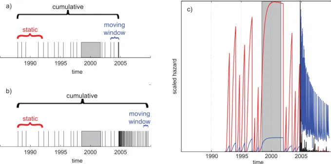
network non-operation as though no repeats occurred during this time, which likely biases our results for the second data set to indi-cate a lower degree of predictability. The static approach explores the question of how much one can learn using only the earliest events in a sequence; the cumulative approach imitates a learning proce-dure and incorporates a maximum amount of information; and the moving-window approach favours the idea that sequences may ex-perience important short-term variations associated with other fault zone phenomena (e.g. the nearby 2004 Parkfield M6 earthquake). We illustrate these three variants with an actual sequence from the second data set in Fig. 2. The strong clustering following the 2004
M6 Parkfield earthquake is apparent in Fig. 2(c), where the static
Figure 2. Illustration of method to construct hazard function, assuming n0= 5. Shaded region in (a–c) denotes period of HRSN non-operation. (a) Time line
of a sequence of repeating earthquakes prior to 2005; vertical lines indicate the occurrence of a repeat. Labels indicate which events are used to determine the best-fit model immediately following the last shown repeat. (b) Same as in (a) but now including all recorded repeats until early 2010. (c) Unit-free hazard functions corresponding to the data and method variants shown in (b), scaled to highlight temporal variation. Static variant shown in red, cumulative in black and moving-window in blue.
variant does not have time to grow between the rapid repeats, and the hazard from the moving-window approach changes drastically. We note that this sequence is not representative of the full range of behaviour of all sequences and is merely meant to demonstrate our methods. We offer sequence data and the codes used in this study in the online supplement (see Supporting Information).
Because we are interested in the general temporal predictability of earthquakes rather than any particular sequence, we concatenated the hazard functions for all sequences end-to-end, and we concate-nated the binned daily number of earthquakes for each sequence end-to-end. We ‘stacked’ the sequences in this way to reduce po-tential selection bias; this procedure guaranteed that we treated all sequences and their repeats equally, and we did not restrict our anal-ysis to sequences with a suspected high degree of periodicity (cf. Goltz et al. 2009). To determine the predictive skill of the concate-nated hazard functions, we examined the correlation between the hazard and the occurrence of repeats: we treated the hazard as an alarm function (Zechar & Jordan 2008) and performed a forecast experiment. In particular, we chose a threshold value, generated a corresponding set of alarms from the hazard function, and then cal-culated the fraction of time occupied by alarms and the fraction of target earthquakes that fell outside of alarm times (the miss rate). For a given threshold value and a given hazard value, an alarm was declared for the following 24 hr if the hazard value exceeded the threshold value. If no repeat occurred on that day, this alarm was counted as a false alarm. By choosing monotonically decreasing threshold values, we traced out a Molchan trajectory that charac-terizes the predictive skill of the alarm function. Molchan (1991) showed that the hazard function gives an unbiased estimate of the number of earthquakes in a time interval and may be optimal in terms of the Molchan diagram—the plot of alarm time fraction and miss rate.
Simply stated, this method quantifies the intuitive measure that hazard should be high just before repeats occur and low otherwise.
We note that the absolute values of the hazard are irrelevant as only the relative magnitude of the hazard is used to generate alarms.
4 R E S U L T S
To maximize the number of target earthquakes in these predictabil-ity experiments, we set n0= 3. (We found that the results are fairly
insensitive to changes to the value of this parameter.) The choice
n0= 3 yielded 524 target earthquakes in the first data set and 743
target earthquakes in the second data set. In Fig. 3, we present the corresponding Molchan trajectories. Here, the diagonal represents no predictive skill and any point falling below the diagonal indi-cates an alarm set that is better than random guessing. We have plot-ted the 95 per cent confidence bounds around the diagonal; points falling outside this region indicate performance that is significantly better (or significantly worse) than random alarms. Because each forecast variant obtains points inside and outside the confidence interval, we simplify the trajectories to a single quantity: the area
A above the trajectory, called the area skill score (Zechar & Jordan
2010).
We test the null hypothesis that the observed area skill score could have been obtained by chance; that is, by declaring alarms at ran-dom. For the given distribution of target earthquakes, we simulate the distribution of area skill scores obtained from random alarms (Zechar & Jordan 2010) and report in Fig. 3 the fractionα of simu-lated area skill scores that exceed the observed area skill score; this is analogous to a p-value. Except in the case of the static approach to the second data set, one can reject the null hypothesis with complete confidence. For the lone exception, the poor predictive performance is primarily caused by dramatically shortened interevent times in the wake of the 2004 M6 Parkfield Earthquake, a phenomenon that was qualitatively predicted by Langbein et al. (2005) as the result of increased loading by after-slip. The suddenly increased repeat rates
Figure 3. Molchan diagram—plot of fraction of time covered by alarms and miss rate—for both data sets and each of the three method variants. Dashed lines
indicate the 95 per cent confidence region about the unskilled diagonal. Circles mark the Molchan trajectory of the static variant; triangles mark the cumulative variant and squares mark the moving-window variant. N denotes the number of target earthquakes in the experiment, A denotes the area skill score for each variant’s trajectory andα denotes the percentage of 1000 random trajectories with an area skill score greater than A. (a) First data set, with 160 sequences and (b) second data set, with 34 sequences.
may also explain the apparent superiority of the moving-window approach to the second data set.
We note that both data sets, despite their many differences, seem to be characterized by a comparable degree of predictability. Nev-ertheless, we make no claims regarding the relative performance of each of the three modelling variants, other than noting that the static approach does very poorly when applied to the second data set.
5 D I S C U S S I O N A N D C O N C L U S I O N S
In this study, we conducted retrospective forecast experiments that demonstrate the temporal predictability of repeating mi-croearthquakes at Parkfield, California. Because these experiments were not fully prospective, we intentionally used very simple mod-elling approaches. For example, our analysis ignores any interaction between sequences or other earthquakes and does not incorporate other available data that could potentially improve forecasts (e.g. from geodetic instruments, the relative sizes of events within se-quences or the regional earthquake catalogue). Moreover, although we checked the robustness of our results with respect to variations in model parameter values, we made very few attempts to optimize our models. Indeed, the minor sophistication of this study—allowing the hazard models to update after each new repeat, and selecting the best model from several functional forms—is likely unnecessary to highlight the inherent predictability of these sequences. (In check-ing the robustness of our method, we also tried variants in which the functional form was fixed, and we obtained comparable results.)
Despite these caveats, we have a simple, quantitative method that allows a fundamental conclusion: the temporal behaviour of these sequences is predictable. However, it is not wholly satisfying to claim a posteriori that, if one had adopted this method, one would have performed better than random guessing (Werner et al. 2010). The logical next step is to determine how to exploit this predictabil-ity in a forward sense, and to begin conducting prospective forecast experiments. One could simply use the best-fit interevent time dis-tributions employed in this study: the cumulative distribution is a direct way to estimate the probability of a repeat within a given period. More sophisticated methods might yield more profound un-derstanding, and future studies should emphasize the development of physical models that might incorporate other geophysical data and that can produce probabilistic forecasts for each sequence. Per-forming more advanced prospective experiments is also important because these sequences are not stationary; in particular, most se-quences exhibited a strong rate increase following the 2004 M6 Parkfield event. Had we only analysed the first data set, which does not include the effect of the 2004 earthquake, one might reasonably conclude that the predictability of these sequences was due to pe-riodicity. However, given that our analyses of both data sets yield similar results, we conclude that the predictability is not simply a result of periodicity, or a result of clustering, but instead a mixture of both processes whose systematics may have a mechanical basis (Nadeau & Johnson 1998; Chen et al. 2007).
The identification of repeating earthquakes is also an important issue, and one that is not merely technical. The seismic moments and other source parameters among events in these repeating sequences are known to vary subtly from cycle to cycle (Dreger et al. 2007; Taira et al. 2009), so to decide that two earthquakes are enough alike that one can be considered a repeat of the other requires that some similarity criteria are satisfied; in other words, this is a model-dependent decision. And the data used to test against these criteria are themselves inherently uncertain. Because we observe some
vari-ation among events in any given sequence, we also cannot say that they are exact repeats. This is seemingly analogous to the sequence of M6 earthquakes at Parkfield, which was (and sometimes still is) treated as a sequence of repeating events, although distinctions between instrumentally recorded events in that sequence are sub-stantial and have specific physical implications (Langbein et al. 2005). Given the need, then, to replace an idealized definition of repeating earthquakes with a more relaxed set of similarity criteria, can we still say something useful regarding temporal predictability of earthquakes (of any size)? If so, this would suggest that the exact details of repeat identification are not particularly important, and it reinforces the idea that learning something about the occurrence of small earthquakes can improve our understanding of the occurrence of large earthquakes.
A C K N O W L E D G M E N T S
We thank Peter Shebalin and Ilya Zaliapin for fruitful discussions, and we thank Yan Kagan for constructive criticism. We thank Masami Okada for sharing results prior to publication. JDZ was supported in part by NSF grant EAR-0944202 and USGS grant G11AP20038. Support for RMN was provided through NSF grants EAR-0738342 and EAR-0910322. The HRSN is operated by the University of California, Berkeley Seismological Laboratory, with financial support from USGS grant G10AC00093.
R E F E R E N C E S
Akaike, H., 1974. A new look at the statistical model identification, IEEE
Trans. Autom. Control, 19, 719–723.
Bakun, W.H. & Lindh, A.G., 1985. The Parkfield, California, earthquake prediction experiment, Earthq. Predict. Res., 3, 285–304.
Beeler, N.M., 2004. Review of the physical basis of laboratory-derived re-lations for brittle failure and their implications for earthquake occurrence and earthquake nucleation, Pure appl. Geophys., 161, 1853–1876. Ben-Zion, Y., 2008. Collective behavior of earthquakes and faults:
continuum-discrete transitions, evolutionary changes and cor-responding dynamic regimes, Rev. geophys., 46, RG4006, doi:10.1029/2008RG000260.
Boettcher, M.S., McGarr, A. & Johnston, M., 2009. Extension of Gutenberg-Richter distribution to MW−1.3, no lower limit in sight, Geophys. Res.
Lett., 36, L10307, doi:10.1029/2009GL038080.
Chen, K.H., Nadeau, R.M. & Rau, R.-J., 2007. Towards a universal rule on the recurrence interval scaling of repeating earthquakes? Geophys. Res.
Lett., 34, L16308, doi:10.1029/2007GL030554.
Chen, K.H., B¨urgmann, R. & Nadeau, R.M., 2010a. Triggering effect of M 4–5 earthquakes on the earthquake cycle of repeating events at Parkfield,
Bull. seism. Soc. Am., 100(2), 522–531, doi:10.1785/0120080369.
Chen, K.H., B¨urgmann, R., Nadeau, R.M., Chen, T. & Lapusta, N., 2010b. Postseismic variations in seismic moment and recurrence interval of re-peating earthquakes, Earth planet. Sci. Lett., 299, 118–125.
Dreger, D., Nadeau, R.M. & Chung, A., 2007. Repeating earthquake fi-nite source models: strong asperities revealed on the San Andreas Fault,
Geophys. Res. Lett., 34, L23302, doi:10.1029/2007GL031353.
Goltz, C., Turcotte, D.L., Abaimov, S.G., Nadeau, R.M., Uchida, N. & Matsuzawa, T., 2009. Rescaled earthquake recurrence time statistics: ap-plication to microrepeaters, Geophys. J. Int., 176, 256–264.
Jackson, D.D. & Kagan, Y.Y., 2006. The 2004 Parkfield earthquake, the 1985 prediction, and characteristic earthquakes: lessons for the future,
Bull. seism. Soc. Am., 96(4b), S397–S409.
Jordan, T.H., 2006. Earthquake predictability, brick by brick, Seismol. Res.
Lett., 77, 3–6.
Langbein, J. et al., 2005. Preliminary report on the 28 September 2004, M 6.0 Parkfield, California earthquake, Seismol. Res. Lett., 76(1), 10–26, doi:10.1785/gssrl.76.1.10.
Molchan, G.M., 1991. Structure of optimal strategies in earthquake predic-tion, Tectonophysics, 193, 267–276.
Nadeau, R.M. & Johnson, L.R., 1998. Seismological studies at Parkfield VI: moment release rates and estimates of source parameters for small repeating earthquakes, Bull. seism. Soc. Am., 88(3), 790–814.
Nadeau, R.M. & McEvilly, T.V., 1999. Fault slip rates at depth from recurrence intervals of repeating microearthquakes, Science, 285, 718–721.
Nadeau, R.M., Foxall, W. & McEvilly, T.V., 1995. Clustering and periodic recurrence of microearthquakes on the San Andreas Fault at Parkfield, California, Science, 267, 503–507.
Schorlemmer, D., Zechar, J.D., Werner, M.J., Field, E.H., Jackson, D.D. & Jordan, T.H., 2010. First results of the Regional Earthquake Like-lihood Models experiment, Pure appl. Geophys., 167(8/9), 859–876, doi:10.1007/s00024-010-0081-5.
Shearer, R., 1985. Minutes of the National Earthquake Prediction Evaluation Council (NEPEC). Open-File Rep, U.S. Geol. Surv., 85–507.
Taira, T., Silver, P.G., Niu, F. & Nadeau, R.M., 2009. Remote triggering of fault-strength changes on the San Andreas fault at Parkfield, Nature, 461, doi:10.1038/nature08395.
Werner, M.J., Zechar, J.D., Marzocchi, W. & Wiemer, S., 2010. Retrospective evaluation of the five-year and ten-year CSEP-Italy earthquake forecasts,
Ann. Geophys., 53(3), 11–30, doi:10.4401/ag-4840.
Zechar, J.D. & Jordan, T.H., 2008. Testing alarm-based earthquake predictions, Geophys. J. Int., 172(2), 715–724, doi:10.1111/j.1365-246X.2007.03676.x.
Zechar, J.D. & Jordan, T.H., 2010. The area skill score statistic for evaluating earthquake predictability experiments, Pure appl. Geophys., 167(8/9), 893–906, doi:10.1007/s00024-010-0086-0.
Zechar, J.D., Schorlemmer, D., Liukis, M., Yu, J., Euchner, F., Maechling, P.J. & Jordan, T.H., 2010. The Collaboratory for the Study of Earthquake Predictability perspective on computational earthquake science, Concurr.
Comp-Pract. E., 22, 1836–1847, doi:10.1002/cpe.1519.
S U P P O RT I N G I N F O R M AT I O N
Additional Supporting Information may be found in the online ver-sion of this article:
Supplement. Sequence data and the codes used in this study.
Please note: Wiley-Blackwell are not responsible for the content or functionality of any supporting materials supplied by the authors. Any queries (other than missing material) should be directed to the corresponding author for the article.