HAL Id: hal-02997100
https://hal.archives-ouvertes.fr/hal-02997100v3
Preprint submitted on 8 Dec 2020
HAL is a multi-disciplinary open access
archive for the deposit and dissemination of sci-entific research documents, whether they are pub-lished or not. The documents may come from teaching and research institutions in France or abroad, or from public or private research centers.
L’archive ouverte pluridisciplinaire HAL, est destinée au dépôt et à la diffusion de documents scientifiques de niveau recherche, publiés ou non, émanant des établissements d’enseignement et de recherche français ou étrangers, des laboratoires publics ou privés.
Trade Liberalization, Income, and Multidimensional
Deprivation in Brazil
Louisiana Teixeira
To cite this version:
Louisiana Teixeira. Trade Liberalization, Income, and Multidimensional Deprivation in Brazil. 2020. �hal-02997100v3�
Trade Liberalization, Income, and Multidimensional
Deprivation in Brazil
Louisiana Cavalcanti Teixeira
University Paris Dauphine, DIAL-IRD
[email protected]
Abstract
The aim of this study is to treat the trade liberalization’s impacts in both monetary and non-monetary conditions. Using the difference-in-differences method and a panel from 1987-1997, the obtained evidence suggests that trade liberalization have differently impacted the labor force within formality and informality; import and export sectors; in terms of income and household’s deprivation. Trade have worsened the average income and implied a deterioration in the household’s multidimensional conditions in the formal sectors and contributed to the labor informalization process already underway, putting in evidence the migration of workers towards informality. Moreover, although the shock of trade harmed more intensely import sectors, export sectors would be expelling skilled better-paid workers to specialize in unskilled lower paid labor. The trade liberalization perpetuated the international division of labor and was unable to permit structural changes capable of adjusting distortions inherent to the national productive structure.
JEL classification: F12, F13, F14.
1
Introduction
Traditional trade theory often emphasizes long-run equilibria in which the reallocation of resources between economic activities is achieved without frictions. These models, endowed with a static character, have given little attention to the adjustment process in the transition from one equilibrium to another, creating a tension between academic economists who support trade liberalization and policymakers concerned with social and labor outcomes (Salem and Benedetto (2013); Hollweg, Lederman, Rojas, and Bulmer (2014); Dix-Carneiro and Kovak (2017)). Frequent changes in cross-sectional household surveys have forced researchers to focus on relatively short intervals to ensure consistency over the periods analyzed (Goldberg and Pavcnik (2007)).
Over the past few decades, expanding literature has been treating globalization and trade’s social outcomes. First for the advanced countries: in the 80s, the policy debate essentially in-volved industrialized countries with rising inequalities and increased international competition in domestic markets. Then, in the 1990s-2000s, for developing countries: the implementation of trade reforms in several developing and emerging economies (e.g., Brazil, Mexico, and In-dia, among others) and the growing availability of databases has led to more studies on the distributional and social effects of international trade in the developing world.
The debate gained relevance regarding income. Some expanding literature has analyzed the links between trade, income inequalities and poverty, becoming one of the most discussed topics in academic and policy circles. The debate on monetary poverty has generally pointed to the conclusion that liberalization generally boosts income in the long run and thus reduces poverty (Winters, McCulloch, and McKay (2004), Winters and Martuscelli (2014); Kelbore (2015); Sofjan (2018) among others). Nonetheless, other studies showed some evidence indicating that regions which were more exposed to trade liberalization experienced smaller reductions in poverty (Castilho, Menendez, and Sztulman (2012); Topalova (2005)). Regarding income inequalities, some authors highlighted the trade’s potential on inequality reduction (Wei and Wu (2001); Ferreira, Leite, and Wai-Poi (2007); Helpman, Itskhoki, Muendler, and Redding (2017) while other studies suggested that trade did not impact income inequalities (Topalova (2005); Sofjan (2018)). Castilho et al. (2012) mentioned that empirical studies that have tried to link trade liberalization and poverty or income inequality show contrasting results, depending on the methodology and country studied.
Authors such as Dollar and Kraay (2004) clarify the trade’s potential on poverty reduction by analyzing a set of developing countries that have globalized after 1980. Most of these economies experienced a remarkable growth process, accompanied by a reduction of absolute1
poverty. Countries that did not experience openness processes did not face a similar pattern of growth. They also stress that during the 1980s and 1990s, ”globalizers” were catching up to rich countries while the rest of the developing world was falling farther behind.
We can link this poverty reduction movement to the export sector. Hoekman, Michalopou-los, Schiff, and Tarr (2001) explore how to implement trade liberalization as a form of strategy to alleviate poverty in developing economies. The authors conclude that there are no examples of economies that have significantly reduced poverty without significantly increasing exports. Examining trade policy models that have reduced poverty permitted the authors to infer that liberalizing trade policies are necessary but not sufficient for growth or poverty reduction.
1Condition where household income is below a necessary level to maintain basic living standards (food, shelter, housing). Comparable between different countries and also over time.
Other studies, such as Harrison (2006), explore the links between globalization and poverty, noting that the poor in the export sectors have benefited from trade and FDI reforms. Chang, Kaltani, and Loayza (2006) also argue about the importance of globalization in increasing per capita income through the labor market flexibility. J. Balat, Brambilla, and Porto (2009) stress that trade gains are benefited by the availability of markets for agricultural export crops. Anderson (2005) analyzes the effects of agricultural trade reforms on poverty reduction in developing countries. According to the author, if developing countries wish to take complete advantage of the Doha Round’ new opportunities, multilateral trade reforms that liberalize the farmers’ product and factor markets are imperative.
Porto (2003), Porto (2006)) finds a poverty reduction effect of trade reforms in Argentina. The author studies the impact on household poverty through the estimation of general equilib-rium distributional effects, using the channel of prices and wage price-elasticities. In his first study, Porto (2003) shows that trade reforms as well as enhanced access to foreign markets has a poverty-decreasing effect; In his second study, Porto (2006) finds evidence of a positive impact on poverty reduction of the Mercosur trade agreement on Argentine families in the 90s.
Nevertheless, using a different methodological approach, McCaig (2011), looking at short run for Vietnamese provinces, finds that between 2002 and 2004 districts more exposed to tariff cuts may have experienced lower declines in poverty while those with increased access to U.S. export markets led to greater drops in poverty. In an analysis about the Indian provinces, Topalova (2005) obtained similar results: using a regional approach, she finds that trade liberalization in the 1987-1997 period led to an increase in poverty but had no effect on inequality in the Indian rural districts. The author also finds no impact of trade exposure on district poverty and inequality in urban India.
Winters and Martuscelli (2014) make a review on outstanding recent literature about the effects of trade liberalization on poverty in developing countries and attempt to identify whether our knowledge has changed significantly over a decade. The reasoning that liber-alization typically boosts income and consequently reduces poverty remains; some authors suggest that this finding is not valid for extremely impoverished countries, but this sugges-tion is far from proven at present. Regarding microeconomics, recent literature also confirms that liberalization has very heterogeneous effects on poor domestic establishments, depending, among other things, on the releasing of specific trade policies and how the family earns its living. According to the authors, literature points that someone working in the export sector predicts gains and someone else working in the import-competing sector predicts losses. New research has suggested that trade increases intra-sectoral wage inequality in several ways, but this research generally does not indicate that the poor lose.
There are different conclusions in different countries. Following Castilho et al. (2012), this fact encourages us to continue a case study that may be of particular interest, re-examining the question for the case of Brazil. While most economists agree that, in the long run, open economies fair better in aggregate than do closed ones, many fear that trade could be detrimental to the poor (Winters et al. (2004)).
The choice of the Brazilian case for the treatment of this theme is due to numerous reasons. First, Brazil liberalized its imports in the 1990s while maintaining certain levels of trade protection (Pereira (2006); Abreu (2004)). At the same time, according to OECD reports, Brazil has been among the emerging countries with promising results in terms of poverty and inequality reduction throughout the past decades. And despite being among the most unequal countries, Brazil has put in place transfer measures (pensions and retirement system, Fome Zero, Bolsa Familia) that have contributed to reducing poverty and inequality. It seems that the gains expected from opening up to international economic dynamisms, accompanied by social programs and transfer measures, have perhaps contributed to poverty reduction in
Brazil.
The availability of very high-quality individual and household datasets, representative of almost the whole country and sectors of activity, covering a period that starts before the trade liberalization, is another relevant point that makes possible an accurate analysis of the Brazilian case. It is therefore possible to establish long, reliable and comparable annual series at the sectorial-level. As often emphasized, within-country studies do not suffer from the long list of data quality problems encountered by cross-countries studies, such as differences in data definitions and collection methods leading to problems of comparability between countries and over time.
Our contribution to the economic literature lies in extending the existing empirical studies on the links between trade and its effects in terms of income, but also adding its non-monetary impacts. Despite the increasingly dissemination of methods in the economic literature in recent years, the existing works have been dealing with the theme of trade and poverty in its monetary form (Ferreira and Barros (2004); Ferreira, Ravallion, and Leite (2010); Castilho, Menendez, and Sztulman (2015); Helpman et al. (2017); among others). There is not to our knowledge any study on the direct relationship between trade and the multidimensional outcomes in Brazil to date. Bringing this thematic to poverty in its multidimensional form becomes an innovative solution to possibly face some of the limits related to the complexity of this issue. Using detailed micro-data across Brazilian states, from 1987 to 1997, we seek to measure whether manufacturing sectors that faced a greater degree of exposure to trade during the opening process in the 90s experienced these effects in terms of income and multidimensional deprivation in different ways. In this investigation, we examine the channels that linked trade to poverty and vulnerability. We analyzed two channels: 1) a direct and 2) an indirect. The first embodies a direct effect of trade, which represents impacts on income. The second denotes an indirect effect, i.e. the effects on the household’s multidimensional conditions, illustrated by the multidimensional deprivation. This indirect influence is represented by the trade impacts on the employees’ standards of living, education and health, which could be interpreted as infrastructure changes, access to consumption and technology (through lower prices amplified by increased competition and product supply) or even indirect earnings outcomes engendered by trade.
Our concern is to treat these issues as a channel analysis to studies on poverty and social development. We find some evidence that could indicate tariff cuts impacted differently the formal and informal sectors. The trade liberalization negatively impacted the formal sector’s average income, contributing to the informalization process already existing and confirming what we have already seen in the Brazilian economic literature (Dix-Carneiro and Kovak (2017); Maloney, Bosch, and Goni (2007)). Regarding the household’s multidimensional con-ditions, trade liberalization also deteriorated the household’s non-monetary conditions within formal activities and benefited informality.
2
The Capability Approach: Multidimensional Poverty
Poverty has long been understood as the lack of sufficient income or consumption to meet a basic living standard. The underlying assumption is that money, as a ”universally convertible asset”, can be ”translated into satisfying all other needs” (Scott, 2002, p. 488). Nonetheless, poverty may arise not only from tight income but also in relation to low levels of education and health, poor access to sanitation, clean water and public services, limited opportunities and freedoms.
The problem of the current debates treating poverty only in its monetary form resides in the fact that it disregards the real household’s conditions and capabilities. Sen (1999)
proposed the capability approach as a conceptual framework of well-being to the poverty discussion. This fact justifies the recent debate’s expansion to the so-called multidimensional poverty (J. F. Balat and Porto (2005); Barros, Carvalho, and Franco (2006); Alkire and Santos (2011); Alazzawi (2013), Fahel, Teles, and Caminhas (2016)). Despite the limitations of existing studies on this non-monetary measure, the poverty as a multidimensional phenomenon has been widely diffused in the scientific environment in recent years. The complexity of the channels through which globalization affects inequality as well as poverty within a country partially motivated the debate (Goldberg and Pavcnik (2007); Winters et al. (2004); Ferreira et al. (2007), for a survey on the various trade-transmission mechanisms).
Since the 1990’s we can identify this evolution of social-institutional thinking through the UNDP Human Development Report, which shifted the focus from poverty analysis to the human development approach. According to the UNDP, the process of expanding individual choices characterizes human development. In this perspective, if human development means the expansion of choices, in poverty there is a denial of more basic opportunities, interfering with the attainment of a long, healthy and creative life (UNDP, 1997). This new paradigm of conception of poverty has been expanding its acceptance in the world along with the use of the conceptual and measurable parameters of multidimensional poverty and it has been increasingly influencing the design and implementation of public social policies. In particular, in Brazil and in Latin America, one can observe the manifestation of these trends, mainly through the reconfiguration of their social protection systems.
In recent years, increasing literature has been treating poverty on its non-monetary form. Nonetheless, in terms of the links between trade and the multidimensional poverty, economic studies remain limited. In this restricted literature, some authors sought to compare the monetary and the non-monetary poverty indicators. Using monetary and non-monetary panel data from 1998-2006, Alazzawi (2013) investigate the dynamics of poverty and the impact of trade liberalization on poor and low waged workers in Egypt. The authors find a relatively low level of economic mobility in both income and non-income indicators, with the majority of those who were ”poor” in 1998, whether in the monetary or non-monetary dimension, remaining so by 2006. Trade reforms though tariff cuts and increased export promotion exerted a small positive influence on the poor’s incomes; however, the greater the informalization of the workers and the higher the incidence of low quality jobs have been observed. The authors also find greater gender inequalities among the private sector workers.
Zhang (2016) has expanded the analysis to the Chinese case. Using data from the China Health and Nutrition Survey (CHNS), covering the years 1989-2011, the author explains and applies the Alkire and Foster Method (AF Method) to examine and compare multidimensional and monetary poverty in China. The study points that China’s multidimensional poverty has declined dramatically from 1989-2011. Reduction rates and patterns, however, vary by di-mensions: multidimensional poverty reduction exhibits unbalanced regional progress as well as varies by province and between rural and urban areas. In comparison to income poverty, multidimensional poverty reduction does not always coincide with economic growth. This re-sult is corroborated by Santos, Dabus, and Delbianco (2019) who argue that economic growth has a far more significant impact on reducing income poverty than on reducing multidimen-sional poverty.
Ezzat (2017) explores the effects of trade openness on multidimensional poverty in Middle East and North Africa (MENA) countries. Using a dynamic panel model, the author sup-ports that trade openness restricts the efforts to alleviate multidimensional poverty in MENA countries. This model highlights the need for governments to provide complementary policies aimed at bringing the benefits of trade openness to those in extreme poverty.
There are different conclusions in different countries. This fact encourages us to examine the Brazilian case.
In Brazil, after the 1988 Constitution, the government adopted a new paradigm of social policies based on social rights, which meant a radical change from the traditional view of social assistance used until then and led to the implementation of several innovative social programs (Vaitsman, Andrade, and Farias (2009); Fahel et al. (2016)). Since then, the social protection system has expanded its coverage to the vulnerable population through the creation of policies and programs that promoted greater social inclusion in the country (pensions and retirement system, Fome Zero, Bolsa Familia). Almost three decades later, there was a significant reduction in poverty with a positive impact on social inequalities. These results are also associated with the price stability, reached in the mid-1990s, the trade liberalization and the economic growth that has occurred, especially in the last decade (Fahel et al., 2016, p. 3). However, the criteria for measuring poverty were traditionally restrictive because they took into account only economic aspects and did not adopt a more comprehensive approach. Only recently, and mainly driven by the implementation of several social programs starting from the 1990s, did the Brazilian government adopt the principle of multidimensional poverty, reconfirming its eligibility criteria and its portfolio of social measures and proposing new challenges for the design and implementation of policies in the country. A proposal for greater assimilation and use of the Multidimensional Poverty Index (MPI) can be seen from this period on Fahel et al. (2016).
3
Trade Liberalization, Income and Poverty in Brazil
in the 90s
In the late 1980s and early 1990s, Brazil was experiencing an economic and inflationary cri-sis. The country, then, adopted various reforms to promote macroeconomic stabilization and overcome this pessimistic scenario. This period was marked by the implementation of a new adjustment policy strategy, with some structural reforms strongly influenced by the recom-mendations of the Washington Consensus, which identified a number of measures deemed necessary for developing countries to create an economic and institutional environment con-ducive to entering a path of self-sustaining growth. In this context, the ECLAC’s Structuralist thought which had influenced the Brazilian policy since the 1950s suffered a significant weak-ening, resulting in a liberal thinking ascension for the ECLAC in the 90s.
The implemented changes in the 1990s included a set of initiatives aimed at inducing a more efficient allocation of resources through external competition and thereby improving the national economic growth performances. Briefly, the proposals led to the promotion of fiscal discipline, commercial and financial liberalization, and the reduction of state participation in the economy.
Regarding the impact of trade liberalization on income and poverty, authors arrive diver-gent conclusions. Using a CGE model, Kume, Piani, and Souza (2003) simulate the impacts of liberalizing policies on employment and on income during the Brazilian liberalization policies in the 90s. The study pointed out that tariff decreases would have positively impacted employ-ment and income. According to the authors, tariff reduction would have led to the devaluation of the Brazilian currency, bringing an improvement in the competitiveness of domestic goods, culminating to an increase on employment and income during this period.
Analyzing the period comprise between 1986 and 2003, Sidou (2007) shows that the in-crease in the export/GDP ratio tended to raise the real income of the 20% most indigent population, reducing inequalities. However, from a regional point of view, he finds different outcomes among the Brazilian regions2.
More recently, using linked employer-employee data, Helpman et al. (2017) find sizable effects of trade on wage inequality in Brazil. Castilho et al. (2015) study the impacts of trade on household income inequality and monetary poverty across Brazilian states from 1987 to 2005, showing that states that were more exposed to tariff cuts experienced smaller reductions in household poverty and inequality. When disaggregating into rural and urban areas within states, the study results suggested that trade liberalization contributed to poverty and inequality increases in urban areas and might be linked to inequality declines in rural areas. Using statistics for formal workers3, Dix-Carneiro and Kovak (2017) study the evolution
of trade liberalization’s effects on Brazilian local labor markets. The authors stress that regions facing more massive tariff reduction experienced prolonged declines in formal sector employment and in earnings relative to other regions. They also state that the impact of tariff changes on regional earnings twenty years after liberalization was three times the effect after ten years. The authors argue that this evolution was due to imperfect interregional labor mobility and other characteristics of the labor demand, driven by slow capital adjustment and agglomeration economies. According to the authors, rather than migrating away, many workers who lose formal employment in negatively affected regions moved to the informal sector in the same region. This mechanism would gradually amplify the effects of liberalization, explaining the slow adjustment path of regional earnings and quantitatively accounting for the magnitude of the long run effects.
Regarding non-monetary poverty, Cruz and Pero (2017) have analyzed the evolution of multidimensional poverty after the 1988 Constitution, from 1985 to 20054. Results show a
continuous decline in multidimensional poverty since 1985, with acceleration after 1995 and better performance in the period from 2003 to 2011. However, from a regional point of view, the authors point out that the decrease in poverty occurred continuously in almost all regions, but with an increase in regional differences - in rural areas compared to urban and metropolitan areas; in the North and Northeast regions compared to the rest of the country. Wealthier regions would have experienced more significant reductions in poverty than poorer regions, intensifying the already existing regional inequalities.
4
Methodology and Data
To empirically analyse the trade liberalization impacts in both monetary and non-monetary social indicators, this analysis exploits two different methods. The first one, model A, uses a difference in differences analysis, where 1987-1988 represents the pre-shock period and 1989-1997 the post-shock. The second one, model B, is a panel model, covering 1987-1989-19975.
4.1
MODEL A: Differences in Differences Model
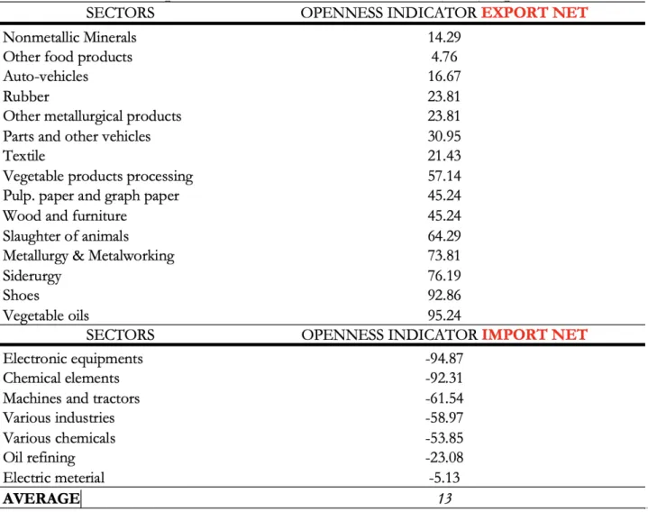
In our study, we considered the sectors most exposed to the liberalization of imports (net im-porters) as our group of treatment and the least exposed (net exim-porters) as our control group. We created an openness indicator in order to define sectors that were more exposed to trade in the period studied, disaggregating net importers from net exporters. As aforementioned, 1987-1988 represents the first period and 1989-1997 the second one, post-event.
South. On the other hand, an increase in imports/GDP ratio tends to reduce inequality in the Country and in the Midwest; nevertheless, worsens the inequality indices in the North.
3Data from the Rela¸c˜ao Anual de Informa¸c˜oes Sociais (RAIS).
4The authors use microdata from 1985, 1990, 1995, 2003, 2011 and 2015 National Household Sample Survey (PNAD/IBGE) to construct multidimensional poverty indicators.
5Model A is used to check the trade impacts in the import sectors in relation to the export sector’s. Subsequently, we keep model B to control the import and export coefficients and the tariffs impacts over time.
Mathematically, the equation for the difference-in-differences method can be represented as follows:
Y = g0 + g1 ∗ d2 + g2 ∗ dB + g3 ∗ d2 ∗ dB + ε (1) where dB, equal to one for individuals in the treatment group (net import sectors) and zero for individuals in the control group (net export sectors); d2, equal to one when the data refer to the second period (1989-1997), post-change, and zero if the data refer to the pre-change period (1987-1988). Y denotes the level of Income/households’ multidimensional conditions. g0 accurately captures the expected value of the studied variable when analyzing the control group before the change, which basically gives us the parameter of comparison. g1 represents the impact of being in the second period on the studied variable (time), g2 the impact of being in the treatment group (net import sectors) on the studied variable, and g3 the post-event impact of the treatment group vis-`a -vis of the control group on the studied variable (which is exactly what we want to discover, i.e., the difference in differences (did) estimator).
4.2
MODEL B: Panel Data Regression Model
The methodology implemented will use the panel data technique, in particular, the estimations by Ordinary Least Squares (OLS) for panel data (pooled OLS).
Here we will present the fixed effects and the random effects models, which are the most used in the economic literature.
4.2.1 Fixed-Effects
The equation for the fixed effects model is defined below:
(2) ln yst = θT arif fs(t−1)+ φImportCoef f icients(t−1)
+ δExportCoef f icients(t−1)+ n
X
j=1
βjlnXjst+ αs+ λt+ εst
where ln yst denotes the level of Income/households’ multidimensional conditions in sector
s at time period t. As it will be described in the data subsection, the multidimensional
deprivation indicator will be used to create the multidimensional conditions variable. In this study, T arif fs(t−1) is the key variable to represent the trade policy while
ImportCoef f icients(t−1)and ExportCoef f icients(t−1)represent the trade flows (lagged6
nom-inal tariff, lagged import and export coefficients). All these indicators represent different ways of capturing the degree of trade exposure of manufacturing sectors.
The vector Xjstincludes j control variables typically assumed to affect levels of income and
households’ conditions. Our main specification includes as controls: the share of individuals by different levels of years of schooling in each sector and the share of the informal workers in each sector (to consider the role of educational differentials and the labor market precariousness).
Finally, αs and λt are the sector and time specific fixed effects respectively and εst is the
error term.
6Regarding the causal relationship between variables, the theory would bring the interpretation that an increase in exports would bring an increase in incomes. However, we cannot make the same interpretation with imports since it could be a reverse causal relation, the increase on incomes that would bring an increase in imports (with increased incomes, we have an increase in consumption and, consequently, an increase in imports). So, in order to create some robustness to this interpretation, we created a panel regression where the explanatory variables are lagged, which means we considered the output for our dependent variable at the following year (1987-1997) from the imports, exports and tariff variations at the previous year (1986-1996).
4.2.2 Random-Effects
The random effects model can be represented as follows:
(3) ln yst = θT arif fs(t−1)+ φImportCoef f icients(t−1)
+ δExportCoef f icients(t−1)+ n
X
j=1
βjlnXjst+ αs+ λt+ ust + εst
The random effects present the same specificities as those illustrated for the fixed effects model. Nonetheless, we add ust which represents the between-sector error.
In order to proceed to our model’s selection, we will perform the Hausman test (between fixed and random effects), and other complementary robustness checks. After proceeding to the Hausman test, we identified the fixed effects method as the most appropriate.
4.3
Data
This study uses different sources of data. The first source is the individual/household level micro-data from the Pesquisa Nacional por Amostra de Domic´ılios (PNAD). It is conducted annually by the Brazilian Census Bureau, the Instituto Brasileiro de Geografia e Estat´ıstica (IBGE)7. PNAD’s micro-data consists of individual and household’s information on the main
socio-economic variables, such as the general characteristics of population, education, labor (covering formal and informal labor), income, housing, migration, fertility, marriage, health, nutrition. The survey samples about 300,000 individuals per year and it is nationally repre-sentative, ensuring coverage of both rural and urban areas of all states of the federation.
The imperfect intersectoral labor mobility within industry sectors observed during this period made us chose to use the manufacturing sectors level, obtained by the aggregation of the individual level information8. The purpose is to check how the trade would have impacted
sectors more exposed to the liberalization of imported goods, as a continuity to the debates on the structural changes that occurred in the industry during the decade. To proceed to this aggregation, we considered the head of household’s information and sector of occupation, keeping the average income and the average multidimensional deprivation index9 by the head
of the household’s sector, considering 22 manufacturing sectors, from 1987 until 199710.
Income is defined as the gross monthly individual monetary income, measured in 2015 Brazilian Reais (BRL R$)11. A major issue when using income information is the quality of
income data, which usually includes measurement errors and outliers, often more prevalent at
7There have been two years in which the PNAD was not carried out during the period of analysis: in 1994 for budgetary reasons and in 1991, because it was a census year.
8By this period, we may observe an increase in more unstable or precarious occupations (increased un-employment rates, informality and expansion of the tertiary sector in total occupation) due to an imperfect intersectoral labor mobility within industry sectors, driven by slow capital adjustment and a generalized de-crease on labor demand (see Freguglia, Teles, and Rodrigues (2002); Correa (1996).
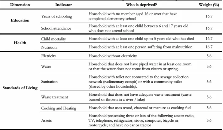
9The multidimensional deprivation indicator will be defined in Appendix A. It will be used to create the household’s multidimensional conditions variable.
10From 1995 on, there has been a change in the classification of the sectors of economic activities, which began to use the classification of CNAE (National Classification of Economic Activities). Thus, we have adapted the old classification to the new one, being guided by the correspondences provided by the CONCLA-IBGE (National Classification Commission); We chose to treat the period from 1987-1997 in order to capture only the effects of the liberalizing shock that occurred between 1988 and 1994, thus seeking to isolate possible reverse effects from crises in the world scenario from the second half of the 1990s.
11Monetary values are deflated to 2015 prices using the IBGE deflators derived from the INPC national consumer price index (see Corseuil and Foguel (2002); Cogneau and Gignoux (2009)).
the two tails of the distribution. A common practice is to simply trim a specific number or percentage of observations at the top and bottom of the income distribution12.
The second data source used to increase the robustness of the monetary results was the individual level micro-data from the RAIS (Rela¸c˜ao Anual de Informa¸c˜oes Sociais)13, a
socio-economic information report requested by the Brazilian Ministry of Labor and Employment to legal entities and other employers annually (covering only formal labor). It represents an essential governmental instrument that aims to respond to the need to monitor labor activity and to provide data for the compilation of statistics and the availability of labor market information. We used the manufacturing sectors level as for PNAD, obtained by the aggregation of the individual level information. However, instead of considering only the head of household’s information we considered all the individuals.
The advantage of working with both RAIS and PNAD lies in the fact that while RAIS brings us a more robust and broad sample of the formal market, PNAD allows us to assess data from both formal and informal sectors. A comparison between the two databases results’ might bring greater robustness to our conclusions. Results for RAIS will be presented in Appendix D.
The third data source is the International trade data provided by the Brazilian Foreign Trade Study Center, the FUNCEX - Funda¸c˜ao Centro de Estudos do Com´ercio Exterior, and the SECEX (MDIC) - Secretaria de Com´ercio Exterior (Minist´erio do Desenvolvimento, Ind´ustria e Com´ercio Exterior). We use the foreign trade statistics, Imports, Exports and Nominal Tariffs, with sectoral breakdown, from 1986 until 199614.
We constructed the Import and Export coefficients using the data for the level of sectoral production, from the PIA (Pesquisa Industrial Anual) provided by the Brazilian Census Bu-reau, the Instituto Brasileiro de Geografia e Estat´ıstica (IBGE), from 1986-1996. The PIA investigates information regarding products and services produced by the national industry. The openness indicator has been created using these variables, which was used to determine the sectors more exposed to the import’s liberalization15.
4.4
Variables description
The choice of the dependent variables used in the study seek to identify whether the house-hold’s multidimensional deprivation responded better to poverty reduction than income changes through trade. Hence, the dependent variable took these forms:
For the ”Difference-in-Differences” estimations (model A)
1. Income: the head of household’s income16 (PNAD - IBGE).
12Castilho et al. (2015), based on Hoffmann and Ney (2008), conclude that the proportion of households declaring zero income in the Census is suspiciously larger than in the PNAD. They also report some very extreme income values at the very top. They end up trimming all zero incomes as well as observations with household incomes over R$ 30,000 in 2000 Brazilian Reais (BRL R$). We followed the same procedure, trimming all zero and individual incomes over R$ 50,000 in 2015 Brazilian Reais (BRL R$).
13Basic data is collected on each individual in the household, in a sample of over 35 million individuals. In order to facilitate the data treatment, we collected a random sample of 20% of the universe of 35 million people, totalizing a new sample of 7 million individuals.
14As we considered the output (y: 1987-1997) at the following year from the imports, exports and tariff variations, the trade data we will use covers 1986-1996.
15The openness indicator will be defined in Appendix B
16Monthly income of the head of household - defined by the highest income family member. Monetary values were deflated based on year 2015.
2. Household0s M ultidimensional Conditions: (1 - the household multidimensional
de-privation indicator) (censored considering poor & vulnerable). In order to proceed to this sectoral aggregation, we considered the head of household’s occupation and its related sector
s (Self elaboration with data from PNAD - IBGE).
A positive coefficient indicates improvements on income levels and in the household’s mul-tidimensional conditions - through a reduction on deprivation17 -, while a negative coefficient
illustrates deterioration to both monetary and non-monetary measures.
For the ”Panel” estimations (model B)
In model B we will use the same variables used in model A. However, in a second moment we will disaggregate our variables in formal and informal sectors. Accordingly, the dependent variable took these forms:
1. Incomest: the head of household’s income , that worked in sector s during the period t
(PNAD - IBGE).
2. Income F ormal & IncomeInf ormalst: the head of household’s income within formality
& the head of household’s income within informality, for sector s and period t (PNAD - IBGE). 3. Household0s M ultidimensional Conditionsst: (1 - the household multidimensional
deprivation indicator) (censored considering poor & vulnerable), for sector s and period t. In order to proceed to this sectoral aggregation, we considered the head of household’s occupation and its related sector (Self elaboration with data from PNAD - IBGE).
4. Household0s M ultidimensional Conditions F ormal & Household0s M ultidimensional Conditions Inf ormalst: (1 - the household multidimensional deprivation indicator) for sector
s and period t, with the head of household within formality, & (1 - the household
multidi-mensional deprivation indicator) for sector s and period t, with the head of household within informality (Self elaboration with data from PNAD - IBGE).
For the opening indicator’s proxy, we added explanatory variables that are representative of the effective opening observed. We also added the control variables described below.
a) Import coef f icients(t−1): The ratio import18 (FUNCEX) / production19 (PIA-IBGE)
(M/P) for sector s in period t − 1;
b) Export coef f icients(t−1): The ratio export20 (FUNCEX)/ production (PIA-IBGE)
(X/P) for sector s in period t − 1;
c) N ominal T arif fs(t−1): Nominal Tariff21 (SECEX) for sector s in period t − 1.
Controls included: Fixed Effects: sector and time; share by levels of years of schooling
by sector; share of informal workers by sector.
4.5
Descriptive Statistics
Table 1 shows some descriptive statistics of the data used in the study. It describes the values assumed by the head of households for each variable in the study. In order to perform our log-linear analysis, being able to include zero values in the statistics and avoid any type of problems related to it, we proceeded a log(x+2) transformation.
17An improvement in the conditions of vulnerable households, which would be experiencing a decrease in deprivation levels among the ten indicators evaluated.
18Industry sectors’ import values (FOB). 19Gross value of industrial production. 20Industry sectors’ export values (FOB).
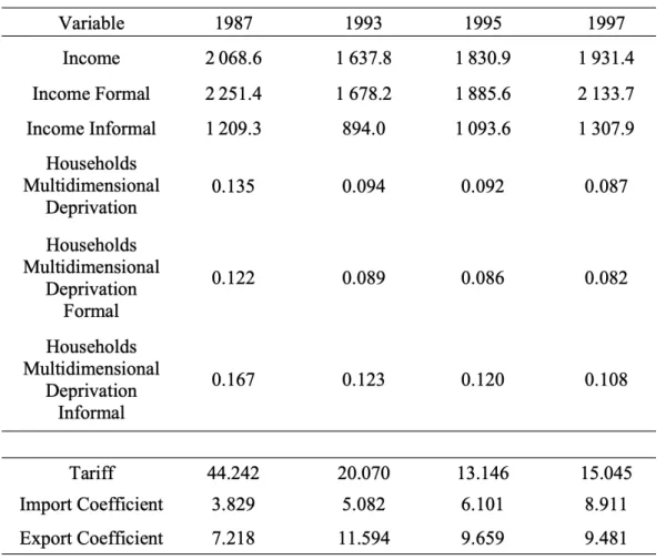
Table 1: Descriptive Statistics - Income (in 2015 R$), deprivation and trade variables
Self-Elaboration.
Table 2 illustrates how real wages, household’s multidimensional deprivation and trade flows evolved between 1987-1997. When evaluating real wages, we may perceive a movement of loss of the average income’s real value between 1987 and 1993 within formal and informal activities. This reality could be justified by the scenario of hyperinflation experienced by the Brazilian economy before the stabilization plan of 1994, accompanied by the trade liberaliza-tion side effects. However, since 1995, there has been a significant improvement in the average income’s value, specially within informality, which could be signaling the informal sector’s expansion. This growth could be justified by the end of hyperinflation, industrial structure changes and the increase in the share of skilled labor. Regarding the average deprivation evo-lution over the period, we can observe an improvement in the household’s conditions through a decrease in the average multidimensional deprivation index, especially between 1987 and 1993. Despite income’s losses and the negative effects of hyperinflation, household’s conditions were prospering. This might be due to certain social advances experienced through the adoption of redistributive policies in the post-1988’s Constitution and the access to consumption driven by the liberalizing policies of the 1990s.
When considering the trade openness indicators, we may perceive a decrease in nominal tariff values, specially between 1987-1993, illustrating the trade liberalization policies adopted by this period. Nonetheless, this trend is slightly reversed between 1995-1997. Regarding the trade flows, we can observe a general growth in the import coefficient over the whole period. In terms of the export coefficient, this positive trend was perceived only between 1987-1993, suffering a drop from 1995 on.
Table 2: Average income (in 2015 R$), deprivation and trade outcomes (1987-1997)
Self-Elaboration.
5
Empirical Results
In this section we will present the empirical results for model A (difference-in-differences) and model B (panel).
5.1
(MODEL A) Difference-in-Differences
The first estimations to be presented correspond to model A and consists of a difference-in-differences analysis. In this estimation, the results are observed for two groups for two periods. The treatment group is exposed to a ”shock” in the second period, but not in the first. The control group is not exposed to the shock either in the first or in the second period.
In our study, we use the manufacturing industry sectors’ level, considering the heads of household’s information on their sector of occupation. Sectors that were most exposed to import liberalization (net importers) were taken as our treatment group and the least exposed (net exporters) were considered as the control group. We distinguished two periods related to the shock (liberalization): the first one going from 1987 to 1988 and the second one (the incidence period), from 1989 to 1997.
Through model A, we intend to verify how trade would be affecting the sectors most exposed to the import liberalization policies (net importers) in relation to the least exposed (net exporters). Thus, we will use model A only initially, keeping model B to the rest of our analysis, in order to control the import and export coefficients as well as the tariffs impacts over time.
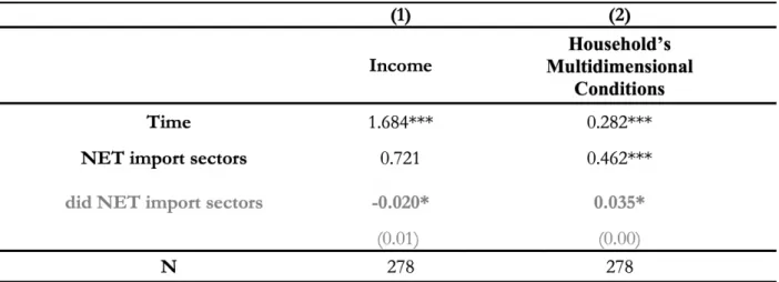
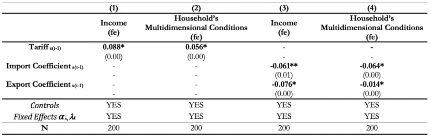
The estimated parameters are presented in table 322.
Table 3: Trade’s Outputs on Income & Multidimensional Conditions Differences-in-differences Regressions (1987 - 1997)23
Source: Self-Elaboration based on PNAD data. Notes: Regressions are weighted by the square root of the number of people in a sector. * p < 0.10; ** p < 0.05; *** p < 0.01. As shown in the first regression (1) for did NET import sectors, results suggest that be-ing an employee in a net import sector durbe-ing the liberalization policies in the 1990s implies a smaller level of real income at 2% if compared to employees in the net export sectors. These findings are consistent with the existent literature conclusions24. In terms of the house-holds’ conditions estimation (2), considering did NET import sectors, we observed a positive coefficient25, indicating that import sector’s employees faced a sharper improvement in the
households’ conditions - i.e, a greater decrease in the level of deprivation of vulnerable house-holds - if compared to those from net export sectors, despite the worst income performances. As importers consisted of sectors with higher technological content, better paid and skilled labor, while exporters were traditional sectors (raw materials, commodities and non-durable consumer goods), it’s feasible to expect that import sectors workers would enjoy from less vul-nerability when compared to workers in export sectors (Kupfer, Ferraz, and Iooty (2003))26.
22In addition to the did estimator ”did NET import sectors”, the model presents ”Time” and ”NET import sectors (Treated)” estimators. ”Time” represents the impact of being in the second period on the studied variable and ”NET import sectors” the impact of being in the treatment group on the studied variable. Thus, being in the second period (1989-1997) implies better household’s conditions at 28.2% and a greater level of income at 168.4% if compared to the first period (1987-1988). Being in the treatment group (net importers) implies better multidimensional conditions, at 46.2% and a greater level of income at 72.1% if compared to the control group (net exporters).
23Results from the PNAD data. Results from the RAIS data regressions are given in Appendix D.
24Literature points that working in the export sector predicts gains and working in the import-competing sector predicts losses (Winters and Martuscelli (2014)).
25Recalling that a positive signal coefficient indicates an improvement in the household’s situation through a drop in deprivation levels.
26Staveren, Elson, Grown, and Cagatay (2012) put light the center-periphery divergence trend. According to the theory, developing countries specialize in labor-intensive low skilled export production while center economies specialize in technology, resulting in significant discrepancies between the import and export sectors’ labor force within each country.
5.2
(MODEL B) Panel Data
In model B, we proceed with the aggregation of a combination of time series and cross-sectional observations multiplied by T periods of time (T=11, for a panel 1987-1997). While the differences in differences model has the advantage of comparing the impact of the shock between the most and the least exposed to the trade liberalization policies, the panel estimation will be able to enjoy a great amount of information to evaluate the sectorial trade impact evolution and with additional degrees of freedom.
5.2.1 Aggregating Formality and Informality
When considering all workers within formal and informal sectors, we first regressed in four different equations - deprivation and income against different measures of trade openness -tariff, Import and Export coefficients. We obtained the following results27:
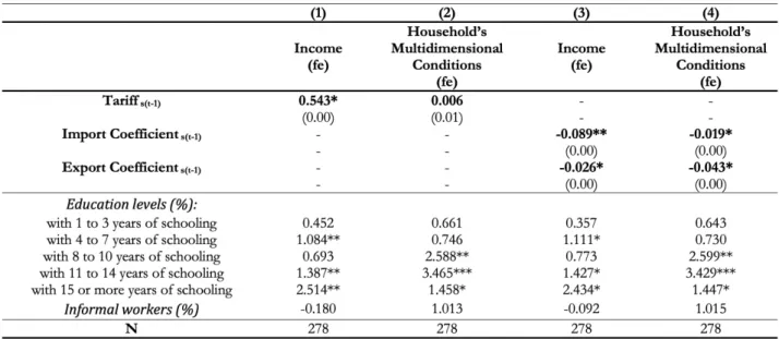
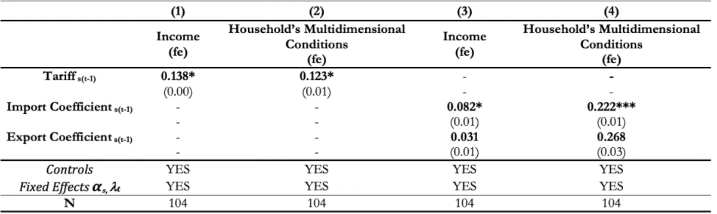
Table 4: Trade’s Outputs on Income & Multidimensional Conditions Panel Regressions (1987 - 1997) (Fixed Effects Model)
Source: Self-Elaboration based on PNAD data. Notes: Standard errors (in parentheses) are robust to heteroskedasticity. All regressions include sector fixed effects and year dummies. Regressions are weighted by the square root of the number of people in a sector. * p < 0.10;
** p < 0.05; *** p < 0.01.
As indicated by the Hausman test, the fixed effects method was determined to be the most appropriate (i.e., that gives more efficient and consistent results).
Analyzing the effect of nominal tariffs in regressions (1) and (2), we obtained a positive and significant impact for income and for the household’s conditions estimations, showing that an increase in the tariffs would lead to an improvement in the level of income and in the multidimensional conditions. When analyzing the coefficients for imports and exports in regressions (3) and (4), we observed a negative and significant relation regarding income and the household’s multidimensional conditions, indicating that increased trade flows implied a worsening in income levels as well as in the non-monetary conditions.
27In order to observe whether the stabilization plan of 1994 led to a structural change in the domestic market, which could have influenced the labor sensitivity to increased trade exposure, we present in Appendix C an empirical analysis of the trade effects before and after the Real Plan.
The evolution of the income estimations - (1) and (3) - may be explained in part by the competitive environment brought by the trade liberalization policies. The industry efforts in response to the increased competition from the process of opening to imported goods involved the organizational and productive restructuring of companies, responded by the downsizing of personnel28. The result would be a notable reduction in the level of employment in the sector,
and a negative impact on the level of income29 (Ramos and Reis (1997); Cirera, Willenbockel,
and Lakshman (2014); Dix-Carneiro and Kovak (2017)).
Considering exports, a positive effect on income is expected. However, the negative result can be due to the evolution of the production that correspond to the denominator of the export coefficient. The rising unemployment, negative production pressures and worst working conditions observed at this time could have negatively impacted the level of earnings. It would be feasible to expect that an increase in exports would not have been enough to compensate for the reverse effects of the downward trend in employment experienced at this period, explaining the negative estimations obtained. Moreover, in our sectorial analysis, income changes are primarily due to an intra-sectorial composition effect (skilled v.s. unskilled labor). As a country’ labor structure depends on the trade specialization of an economy, the negative parameter might be also indicating the replacement of skilled by unskilled labor in export sectors. Kupfer et al. (2003), in a study about the Brazilian economy, emphasized the rapid evolution of the import coefficient in industries with higher technological content and higher income elasticity, and the increase in the exports coefficient in traditional sectors, with low technological content and lower income elasticity. Thus, export sectors in Brazil would be specializing in less qualified lower paid labor to the detriment of skilled better paid workers, creating a negative intra-sectorial composition effect on income levels.
The greater exposure to liberalization would also lead to a deterioration in the households’ conditions, as shown in regressions (2) and (4). Pressures towards lower prices amplified by increased competition and increased product supply would not be compensating for the down-ward trend observed in the labor market by this period, negatively impacting non-monetary conditions.
In the estimation of our equations we included a few control variables that are considered to be usual determinants of income and household’s conditions. Concerning our income and the non-monetary conditions results in table 4, most of the controls are significant and have the expected signs. Education increases income levels and improves the households’ conditions at practically all levels of education. Nonetheless, an increase in the share of informal workers lowers income levels but improves the households’ conditions, going in the opposite direction to what would be expected when considering the non-monetary outcomes. Thus, in the following section we will try to understand intra-sectoral changes - considering formality v.s informality - that could clarify the parameters obtained for the share of informal labor.
28In the ECLAC’s debates on the central and peripheral countries, the development of an industry with high technological content, capable of alienating a country from its peripheral condition, would be its only way out to allow this country to face a competition environment brought by trade liberalizing policies. Despite the development of a considerable industry during the import substitution period, income dropped in the ’90s after trade liberalization. Despite having guaranteed the development of high technological content industries such as in the aeronautics sector, the process of import substitution privileged the intermediate and capital goods industries, failing to finalize the development of the durable consumer goods industry.
29As it will be explored later, it negatively affected formal sector employment and earnings and contributed to an expansion in the informal sector activities. However, Dix-Carneiro and Kovak (2017) point out that the secular ten percentage point contraction of formal employment across the 1990s suggests other forces at play. The authors establish that trade liberalization played a relatively small part in this increase but find suggestive evidence that several dimensions of the Constitutional reform, in particular, regulations relating to firing costs, overtime, and union power, explain much more. The authors then suggest both effects work mostly through the reduction in hiring rates, confirming the importance of labor legislation to firms’ decisions to create new formal sector jobs in Brazil.
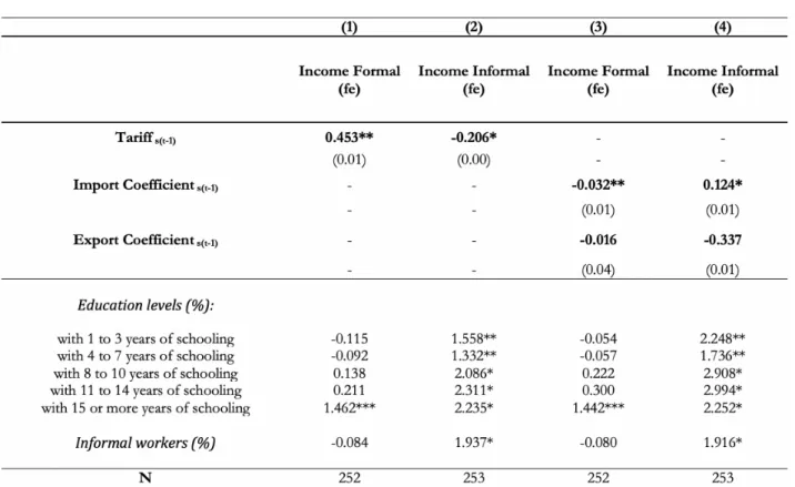
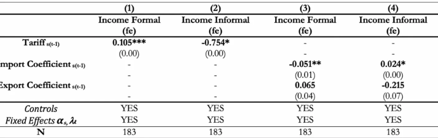
5.2.2 Disaggregating Formality v.s Informality
When disaggregating formal and informal sectors (table 30), regressions (1) and (2) shows that increased tariffs would be protecting income levels in formal sectors while its decrease permitted the income expansion in informal activities. Regressions (3) and (4) illustrate that a rise in the import coefficient implied a reduction in income levels within formality while income expansion within informality. Hence, trade liberalization would be worsening income’s conditions in the formal sector, contributing to a growth within informality. A consistent argument emphasizes that the wave of unemployment brought by the increased competition of imported goods within formal sectors would have led to a migration of workers towards informality30 (Dix-Carneiro and Kovak (2017)). The informal sector’s inflation marked a period of informality development within the Brazilian labor31.
Table 5: Trade’s Outputs on Income: Formality v.s Informality Panel Regressions (1987 - 1997) (Fixed Effects Model)
Source: Self-Elaboration based on PNAD data. Notes: Standard errors (in parentheses) are robust to heteroskedasticity. All regressions include sector fixed effects and year dummies. Regressions are weighted by the square root of the number of people in a sector. * p < 0.10;
** p < 0.05; *** p < 0.01.
Analyzing the control variables in table 5, education increases income levels at practically all levels of education. Nonetheless, an increase in the share of informal workers lowers income levels within formality while increases it within informality, confirming that the informality expansion would be contributing to an income inflation within informal activities.
30According to the classical theory (HOS), a country with abundant unskilled labor would specialize in the sectors in which this labor is used intensively. The informalization movement that occurred during this period could be illustrated by this phenomenon.
31For an explanation to the rising informality in Brazilian metropolitan labor markets from 1983-2002, see Maloney et al. (2007).
Table 6 shows the household’s multidimensional conditions. Liberalization brought a de-terioration in the non-monetary conditions in formal import sectors and in informal export sectors. The estimated parameters are presented below.
Table 6: Trade’s Outputs on Multidimensional Conditions: Formality v.s Informality
Panel Regressions (1987 - 1997) (Fixed Effects Model)
Source: Self-Elaboration based on PNAD data. Notes: Standard errors (in parentheses) are robust to heteroskedasticity. All regressions include sector fixed effects and year dummies. Regressions are weighted by the square root of the number of people in a sector. * p < 0.10;
** p < 0.05; *** p < 0.01.
Regarding the nominal tariff, regressions (1), (2) and (3) present positive and significant results, pointing to an improvement in the households’ deprivation conditions from an increase in tariff levels. When analyzing the import coefficients parameters in regressions (4) and (5), we may observe a negative impact within formality while a positive impact within informality, indicating that a rise of import flows harms the formal labor’s multidimensional conditions but benefits informality. Concerning the export coefficients results in regressions (4) and (5), we might perceive a greater vulnerability faced by informal export sectors.
Considering the control variables in table 6, education improves non-monetary conditions at practically all levels of education. However, an increase in the share of informal workers deteriorates the multidimensional conditions within formality while bring advances within informality, also suggesting that the informal sectors expansion contributed to informality development to the detriment of formality.
6
Conclusion
This paper aimed to treat income and deprivation issues as a channel analysis to studies on poverty and social development. The evidence suggests trade liberalization have differently impacted the labor force within formality and informality; import and export sectors; in terms of income and household’s deprivation.
Liberalization would have worsened the average income in the formal sector and con-tributed to the labor informalization process already underway, putting in evidence the migra-tion of workers towards informality (Dix-Carneiro and Kovak (2017); Maloney et al. (2007))32.
Moreover, although the shock of trade harmed more intensely import sectors - as evidenced in our difference-in-differences estimations -, confirming what is pointed out by the economic theory, export sectors would be expelling skilled better-paid workers to specialize in unskilled lower paid labor.
Liberalization also implied a deterioration in the household’s condition within formal activ-ities. Despite what has been already pointed out by the literature on the hypothesis that lower prices amplified by increased competition and increased product supply would permit infras-tructure changes and better access to consumption and technology (Lisboa, Menezes-Filho, and Schor (2010); Zhang (2016)), these positive outcomes would not be compensating for the downward trend observed in the formal labor market by this period, negatively impacting non-monetary conditions of the labor force within these sectors.
These findings are not consistent with the hypothesis that the indirect effects of trade, rep-resented by the household’s deprivation, have probably responded better to poverty reduction - via the improvement in the households’ multidimensional conditions - than income changes through trade. The negative effects of the Brazilian trade reforms outweigh potential gains in both monetary and non-monetary terms, harming formal labor and benefiting the informality expansion. Moreover, the trend towards informalization, unemployment and imbalances be-tween formal and informal, skilled and unskilled labor, would be expressing the limitations of the liberalization reforms in the absence of labor-oriented policies to help workers to adjust33.
32Nevertheless, the period after the Stabilization Plan of 1994 brought some changes to this tendency. While protectionist policies in terms of increasing import tariffs were more effective in protecting income levels and non-monetary conditions, import and export expansion in a scenario of better macroeconomic stability benefited both, formal and informal sectors, through an intra-sectorial composition effect brought by the increasing demand of skilled labor and the elimination of less qualified jobs, benefiting more significantly formal sector workers (Filho and Rodrigues-Jr (2003); Arbache (2003); Giovanetti and Menezes-Filho (2006); Maloney et al. (2007)). For more details about the influence of the Real Plan on the trade liberalization’s monetary and non-monetary impacts, see Appendix C.
33Despite the innumerable redistributive measures implemented by the Brazilian government in the post-1988 Constitution, especially in the first decade of the 2000s, Brazil still has a regressive tax system, which prevents the accomplishment of more in-depth social advances. Moreover, policies of ”positive discrimination” are still weak and premature, not being able to correct social and economic disparities historically developed and entrenched in Brazilian society. The labor market informality is one among the historical examples that are already rooted in Brazil. It has grown considerably in the past years, especially throughout the 1990s and the second decade of the 2000s. Notwithstanding the recent fall in unemployment, this recovery seems to have been accompanied by an increase in the number of workers without a formal contract. There is, therefore, a failure in the process of recovery of the Brazilian labor market in relation to the quality of employment and the existing policies are not being capable of solving the social delay that continues to deepen. In 2018 the number of workers without a formal contract has reached the highest level since 2012. Self-employment, for example, guaranteed the livelihood of almost one in four Brazilians (25.4%). Last year, there were 11.2 million informal employees in the private sector, in addition to 23.3 million people working on their own. The sum of these two numbers surpassed the total number of employees with a formal contract in the private sector (32.9 million). However, unemployment fell in 2018, something that did not happen in three years. The average unemployment rate was 12.3%, against 12.7% in 2017. The significant drop in unemployment was, however, accompanied by informality (IBGE).
By perpetuating the international division of labor34, the trade liberalization was unable to
permit structural changes capable of creating comparative advantages and thereby adjusting distortions inherent to the national productive structure. Hence, it has deepened the already existing imbalances and delays, converging towards the deepening of asymmetries pointed out by the heterodox thought (Prebisch (1950); Singer (1950)).
Accordingly, for a developing economy like Brazil to be able to enjoy the benefits of the international trade, policymakers should carefully design trade liberalization reforms focused in strategic sectors, accompanied by socioeconomic and industrial policies that favor the devel-opment of the national industry and creates intra-sectoral and interregional economic linkages.
34By not following the Prebish’s diagnosis about the deterioration of the terms of trade between developing and developed economies, Latin American countries ended up witnessing the formation of a state model subordinated to a growing process of modernization that undermined cultures to the benefit of national elites tied to international capital (Munari and Cabral (2015)).
References
Abreu, M. P. (2004). Trade liberalization and the political economy of protection in brazil
since 1987 (working paper siti = documento de trabajo ieci n. 8b). Institute for the
Integration of Latin America and the Caribbean IDB-INTAL. Retrieved from https:// books.google.fr/books?id=Hd4rIQHDkjcC
Alazzawi, M., S.and Said. (2013). Dynamics of multidimensional poverty and trade liberaliza-tion: Evidence from panel data for egypt. In V. Berenger & F. Bresson (Eds.), Poverty
and social exclusion around the mediterranean sea. Springer US.
Alkire, S., & Santos, M. E. (2011). Acute Multidimensional Poverty: A New Index for
Develop-ing Countries (ProceedDevelop-ings of the German Development Economics Conference, Berlin
2011 No. 3). Verein fur Socialpolitik, Research Committee Development Economics. Retrieved from https://ideas.repec.org/p/zbw/gdec11/3.html
Anderson, K. (2005). Agricultural trade reform and poverty reduction in developing coun-tries. In Trade Policy Reforms and Development (chap. 9). Edward Elgar Publishing. Retrieved from https://ideas.repec.org/h/elg/eechap/3070 9.html
Arbache, J. S. (2003). Comercio internacional, competitividade e mercado de trabalho:
algu-mas evidencias para o brasil (Tech. Rep.). Rio de Janeiro: Ipea.
Balat, J., Brambilla, I., & Porto, G. (2009). Realizing the gains from trade: Export crops, marketing costs, and poverty. Journal of International Economics, 78 (1), 21-31. Re-trieved from https://ideas.repec.org/a/eee/inecon/v78y2009i1p21-31.html Balat, J. F., & Porto, G. (2005). Globalization and complementary policies: Poverty impacts
in rural zambia (Working Paper No. 11175). National Bureau of Economic Research.
Retrieved from http://www.nber.org/papers/w11175 doi: 10.3386/w11175
Barros, R., Carvalho, M., & Franco, S. (2006). Pobreza multidimensional no brasil. Ipea. Retrieved from https://books.google.fr/books?id=KkayAAAAIAAJ
Castilho, M. R., Menendez, M., & Sztulman, A. (2012). Trade liberalization, inequality and poverty in brazilian states. World Development, 40 (4), 821-835.
Castilho, M. R., Menendez, M., & Sztulman, A. (2015). Poverty and inequality dynamics
in manaus: Legacy of a free trade zone ? (Working Papers No. DT/2015/18). DIAL
(Developpement, Institutions et Mondialisation). Retrieved from https://ideas.repec .org/p/dia/wpaper/dt201518.html
Chang, R., Kaltani, L., & Loayza, N. (2006, August). Openness Can be Good for Growth:
The Role of Policy Complementarities (Working Papers Central Bank of Chile No. 373).
Central Bank of Chile. Retrieved from https://ideas.repec.org/p/chb/bcchwp/373 .html
Cirera, X., Willenbockel, D., & Lakshman, R. W. (2014). Evidence on the impact of tar-iff reductions on employment in developing countries: A systematic review. Journal
of Economic Surveys, 28 (3), 449-471. Retrieved from https://ssrn.com/abstract=
2448758orhttp://dx.doi.org/10.1111/joes.12029
Cogneau, D., & Gignoux, J. (2009). Earnings Inequalities and Educational Mobility in Brazil over Two Decades. In K. S. & F. Nowak-Lehman (Eds.), Poverty, inequality and policy
in latin america. Cambridge MA.: MIT Press.
Correa, P. G. (1996). Abertura comercial e reestruturacao industrial no brasil: deve o estado
intervir? (Textos para Discussao). BNDES.
Corseuil, C. H., & Foguel, M. (2002). Uma sugestao de deflatores para rendas obtidas a partir
de algumas pesquisas domiciliares do ibge (Texto para Discussao No. 897). IPEA.
Cruz, G. F., & Pero, V. (2017). Pobreza multidimensional no brasil: progressos e desafios
pos-constituicao de 1988 (Texto nao publicado). Universidade Federal do Rio de janeiro.
American Economic Review, 107 (10), 2908-2946. Retrieved from https://ideas.repec
.org/a/aea/aecrev/v107y2017i10p2908-46.html
Dollar, D., & Kraay, A. (2004). Trade, Growth, and Poverty. Economic Journal, 114 (493), 22-49. Retrieved from https://ideas.repec.org/a/ecj/econjl/v114y2004i493pf22 -f49.html
Ezzat, A. M. (2017). Trade openness: An effective tool for poverty alleviation or an instrument for increasing poverty severity? (Working Paper). Cairo, Egypt: College of International Transport and Logistics, Arab Academy for Science, Technology and Maritime Transport. Retrieved from http://erf.org.eg/ publications/trade-openness-an-effective-tool-for-poverty-alleviation -or-an-instrument-for-increasing-poverty-severity/
Fahel, M., Teles, L. R., & Caminhas, D. A. (2016). Para al˜am da renda. uma an˜a¡lise da pobreza multidimensional no brasil. Revista Brasileira de Ci ˜ASociais, 31 .
Retrieved from http://www.scielo.br/scielo.php?script=sci arttext&pid=S0102 -69092016000300505&nrm=iso
Ferreira, F. H. G., & Barros, R. P. (2004). The slippery slope: Explaining the increase in extreme poverty in urban brazil, 1976-96. In F. Bourguignon, F. Ferreira, & N. Lustig (Eds.), The microeconomics of income distribution dynamics in east asia and latin
amer-ica (Vol. 1, p. 83-124). The World Bank Oxford University Press.
Ferreira, F. H. G., Leite, P. G., & Wai-Poi, M. (2007). Trade liberalization, employment flows,
and wage inequality in Brazil (Policy Research Working Paper Series No. 4108). The
World Bank. Retrieved from https://ideas.repec.org/p/wbk/wbrwps/4108.html Ferreira, F. H. G., Ravallion, M., & Leite, P. G. (2010). Poverty reduction without economic
growth? explaining brazil’s poverty dynamics, 1985-2004. Journal of Development
Eco-nomics, 93 (1), 20-36. Retrieved from https://doi.org/10.1016/j.jdeveco.2009.06
.001
Freguglia, R., Teles, J. L., & Rodrigues, B. D. (2002). A mobilidade no mercado de trabalho brasileiro: uma visao qualitativa. In J. A. de Paula & E. Alli (Eds.), Anais do x seminario
sobre a economia mineira [proceedings of the 10th seminar on the economy of minas gerais]. Cedeplar, Universidade Federal de Minas Gerais. Retrieved from https://
EconPapers.repec.org/RePEc:cdp:diam02:200239
Giovanetti, B., & Menezes-Filho, N. (2006). Trade liberalization and the demand for skilled labour in brazil. Economia, 7 (1).
Goldberg, P. K., & Pavcnik, N. (2007). Distributional effects of globalization in developing countries. Journal of Economic Literature, 45 (1), 39-82.
Harrison, A. (2006). Globalization and poverty (Working Paper No. 12347). National Bureau of Economic Research. Retrieved from http://www.nber.org/papers/w12347 doi: 10.3386/w12347
Helpman, E., Itskhoki, O., Muendler, M.-A., & Redding, S. (2017). Trade and inequality: From theory to estimation. Review of Economic Studies, 84 (1), 357-405. Retrieved from https://doi.org/10.1093/restud/rdw025
Hoekman, B., Michalopoulos, C., Schiff, M., & Tarr, D. (2001). Trade policy reform and
poverty alleviation (Policy Research Working Paper Series No. 2733). The World Bank.
Retrieved from https://ideas.repec.org/p/wbk/wbrwps/2733.html
Hoffmann, R., & Ney, M. G. (2008). A recente queda da desigualdade de renda no brasil:
analise de dados da pnad, do censo demografico e das contas nacionais (Vol. 10) (No. 1).
Hollweg, C. H., Lederman, D., Rojas, D., & Bulmer, E. R. (2014). Sticky feet: How
la-bor market frictions shape the impact of international trade on jobs and wages. The
World Bank. Retrieved from https://elibrary.worldbank.org/doi/abs/10.1596/ 978-1-4648-0263-8 doi: 10.1596/978-1-4648-0263-8