HAL Id: tel-01225707
https://tel.archives-ouvertes.fr/tel-01225707
Submitted on 6 Nov 2015HAL is a multi-disciplinary open access archive for the deposit and dissemination of sci-entific research documents, whether they are pub-lished or not. The documents may come from teaching and research institutions in France or abroad, or from public or private research centers.
L’archive ouverte pluridisciplinaire HAL, est destinée au dépôt et à la diffusion de documents scientifiques de niveau recherche, publiés ou non, émanant des établissements d’enseignement et de recherche français ou étrangers, des laboratoires publics ou privés.
l’Univers
Jerôme Gleyzes
To cite this version:
Jerôme Gleyzes. L’énergie noire et la formation des grandes structures de l’Univers. Cosmology and Extra-Galactic Astrophysics [astro-ph.CO]. Université Paris Sud - Paris XI, 2015. English. �NNT : 2015PA112076�. �tel-01225707�
Ecole Doctorale 564
Institut de Physique Th´eorique du CEA Saclay
Discipline : Physique
Sp´ecialit´e : CosmologieTh`
ese de doctorat
Th`ese sur travaux Soutenue le 05/06/2015 par
J´
erˆ
ome Gleyzes
L’´
energie noire et la formation
des grandes structures de l’Univers
Directeur de th`ese : Filippo Vernizzi IPhT-CEA Saclay
Composition du jury :
Pr´esident du jury : Francis Bernardeau IAP (Paris)
Rapporteurs : Olivier Dor´e JPL (Etats-unis)
Pedro Ferreira Oxford (Angleterre)
Examinateurs : Christos Charmousis LPT (Orsay)
This Ph.D has been a great adventure, for which I am extremely grateful. It has been a pleasure to share these moments with nice postdocs, such as Marco, Filippo and Juan and other Ph.D students at IPhT: from the old ones, with Alexandre, Julien and Katya, to the newcomers, Guillaume, Andrei, La¨ıs, Soumya, Rapha¨el, Luca, and Thibault, without forgetting my own generation, Antoine, Hanna, R´emi, Yunfeng and Ga¨elle. There are two people that I specially bothered during these three years, and that stand out from the crowd: Benoˆıt and Piotr. Thanks for having the patience to deal with me, I know I can be tiring sometimes. We did share some good laughs though ! Many thanks also to the students at ICTP, like Marko and Gabriele, whom I visited numerous times: I always came back wiser and happier. To Michele, I say thank you for sharing the work, writing notes, and being there to compare our codes.
More seriously, I have learnt a lot from a number of excellent people. In particular, I would like to thank Claudia de Rham, Andrew Tolley, Justin Khoury and Mark Trodden for the time I had with them last summer in the US, where our interactions were very fruitful. I would also like to give many thanks to Pedro Ferreira and Tessa Baker. My visits to Oxford where always enriching, both from a scientific and from a personal level. Finally, I would like to give special thanks to the people that played a crucial role during my Ph.D and have shaped the researcher I am today: Paolo Creminelli, David Langlois, Federico Piazza. The most important of them is Filippo Vernizzi, my advisor. Thanks for always being there to answer my questions, for treating me like an equal, for giving me so many opportunities to travel and present our work, and for guiding me through many aspects of the world of physicists.
Acknowledgements ii List of Figures v List of Tables vi Abbreviations vii Notations viii 1 Introduction 1
2 The Effective Field Theory of Dark Energy 3
2.1 The Unitary Gauge Action . . . 3
2.2 ADM formalism and the Effective Field Theory of Dark Energy . . . 5
2.3 Going from models to the EFT of DE . . . 8
2.4 Stability and theoretical consistency . . . 9
2.5 Evolution of cosmological perturbations . . . 11
2.5.1 Vector sector . . . 12
2.5.2 Tensor sector . . . 12
2.5.3 Scalar sector . . . 12
2.5.3.1 Obtaining the equations. . . 12
2.5.3.2 Interpretation . . . 15
2.6 Conclusions . . . 18
3 Beyond Horndeski 20 3.1 Horndeski theories . . . 20
3.2 General considerations on higher order derivatives . . . 22
3.3 Generalized Generalized Galileons G3 . . . 23
3.4 Hamiltonian analysis . . . 25
3.5 Field redefinitions . . . 27
3.6 Linear analysis and coupling to matter . . . 29
3.6.1 Stability and ghosts . . . 30
3.6.2 Newtonian gauge and Einstein frame . . . 31
3.7 Conclusions . . . 33
4 Predictions for primordial tensor modes 34
4.1 Tensor sound speed and quadratic action . . . 34
4.2 Other operators . . . 37
4.3 Conclusions . . . 38
5 Consistency relations of the large scale structure 39 5.1 Deriving consistency relations . . . 40
5.2 Going to redshift space. . . 42
5.3 Violation of the Equivalence Principle . . . 43
5.3.1 A toy model . . . 44
5.3.2 Estimate of the signal to noise . . . 45
5.4 Conclusions . . . 47
6 Conclusion 48 6.1 Summary . . . 48
6.2 Outlook . . . 49
A Essential Building Blocks of Dark Energy 58
B Single-Field Consistency Relations of Large Scale Structure Part II:
Resummation and Redshift Space 87
C Single-Field Consistency Relations of Large Scale Structure Part III:
Test of the Equivalence Principle 103
D Healthy theories beyond Horndeski 120
E Resilience of the standard predictions for primordial tensor modes 126
F Exploring gravitational theories beyond Horndeski 132
2.1 The unitary gauge . . . 4
2.2 Geometrical quantities . . . 5
5.1 Unequal time correlators . . . 41
5.2 Equivalence Principle violation . . . 44
5.3 Limits on α2 . . . 46
2.1 Understanding the αi . . . 9
GR General Relativity
EFT of DE Effective Field Theory of Dark Energy EOM Equation(s) Of Motion
DOF Degree(s) Of Freedom
FLRW Friedmann-Lemaˆıtre-Roberston-Walker ADM Arnowitt-Deser-Misner
EP Equivalence Principle WEP Weak Equivalence Principle EFTI Effective Field Theory of Inflation
Φ 00 part of the metric
Ψ trace of the spatial metric
fA≡ ∂A∂f
ϕµ≡ ∇µϕ,
ϕµν ≡ ∇ν∇µϕ, . . .
X ≡ ϕµϕµ
R≡(3)R When not specified, the Ricci scalar is the spatial one.
Introduction
I feel particularly lucky to have been working on my Ph.D at such an exciting time for cosmology. With the fantastic results of the Planck mission [1], our picture of the Universe and its history has become much clearer. The precision of these observations, as well as that of future large scale structure missions such as EUCLID [2] and LSST [3], has also highlighted the challenges that cosmology faces. One of them is that theorists need to build efficient ways to compare theory and observations to say anything quantitative about potential deviations from the standard model of cosmology, ΛCDM. Secondly, to make sure no theoretically consistent model is overlooked, the conditions to have stable theories need to be further investigated. These are the two ideas that fueled my research during my Ph.D.
In particular, this has led me to develop a way to parametrize deviations from ΛCDM at the level of linear perturbations, which is called the Effective Field Theory of Dark Energy (EFT of DE). While the background evolution of the Universe is now quite constrained by distance measurements, much less is known about the evolution of the inhomegeneities that give rise to the large scale structure. Studying their behavior in the linear regime, where theoretical control is still reachable, should prove very informative. I will show in Chapter 2 that the EFT of DE allows for a systematic and quantitative exploration of deviations from ΛCDM, because of its model independence and minimal number of parameters.
While working on the EFT of DE, we realized that what was thought to be the largest class of stable theories for gravity plus a scalar, Horndeski theories [4], could actually be extended. Usually, the stability of theories is obtained by imposing that the equations of motion do not contain terms with more than two derivatives. In Chapter3, I will argue that this is actually not a necessary condition for scalar-tensor theories. This means that before discarding higher derivatives theories, a more careful analysis needs to be performed. As we shall see, this opens the gate to new models.
Although most of cosmology has been focused on scalar perturbations since they have been actually observed, the precision reached by BICEP2 [5] seems to indicate that detecting primordial gravitational waves might well be within our grasp. They are potentially a great source of information on the early universe, since the standard pre-dictions for tensor modes from inflation give straightforward access to its energy scale.
In Chapter 4, I will present why, contrarily to the scalar case, the predictions for ten-sor modes are very robust. In particular, this implies that it is difficult to get a scale invariant power spectrum for gravitational waves without a period of inflation.
The final subject that I will discuss is the work I have done on consistency relations. These relations allow to express (n + 1)-point correlation functions of the cosmic density fields in term of the n-point ones in the limit where one density field is slowly varying in space. As I will show in Chapter 5, their strength comes from the fact that very little information on the n others fields is needed: only that they have Gaussian initial conditions and that they obey the Equivalence Principle. This is a huge advantage since taking correlation functions in the large scale structure typically requires to deal with non linear evolutions that are hard to control theoretically. This control is further lim-ited by the poorly known relation between the galaxy distribution, that we observe, and the underlying dark matter distribution, that we predict. The lack of an accurate under-standing of these phenomena reduces the amount of information that can be extracted from galaxy surveys. Since consistency relations do not rely on the knowledge of short scales physics, they do not suffer from this problem. In particular, this gives access to new ways of testing the Equivalence Principle on very large scales, where gravity is less tested.
In this thesis, I have chosen to present the main results of my work and to emphasize the intuition behind those results, as well as their physical implications. This is why I have tried to keep things short in the main text. Any potential thirst for technical aspects can be quenched by the full articlesA–Gat the end of this thesis.
The Effective Field Theory of
Dark Energy
When looking at alternatives to the standard ΛCDM+GR model, the simplest and most common way is to introduce an extra scalar field (see [6] for a review). It can either act as an additional dark energy fluid, or as a modification of the laws of gravity themselves. It is the easiest modification one can make and is as such the first that should be explored: there is only one additional degree of freedom to consider, making it an informative step before looking at more complicated scenarios. Even in some cases where multiple degrees of freedom are added, such as in massive [7] or bimetric gravity [8] for example, one recovers the case of a single scalar field in relevant limits.
This universality is yet more manifest for a second reason. The goal of the modifications at hand are to try and explain the current accelerated expansion of the Universe [9,10]. Thus, in general, any field added for this purpose will have a background value that is time dependent, since the homogeneous Universe evolves in time. This explicitly breaks the time diffeomorphism invariance, that can be restored as usual with Goldstone modes, which would be a single scalar in this case (see for example [11]). Therefore, the low energy perturbations around a time dependent background will generically be described by this scalar, regardless of the fundamental origin of the theory.
These ideas were first developed in the case of inflation in [12] under the name of the Effective Field Theory of Inflation and then used for example to compute higher order correlation functions, which allow to probe non-Gaussianities [13, 14]. Later, it was applied in the context of late time acceleration in the Effective Field Theory of Dark Energy (EFT of DE) in [15,16] and also [17].
In this section, I will present the concepts behind such an approach as well as its many advantages, based on the work I did in [GLPV1], later summarized in a review [GLV].
2.1
The Unitary Gauge Action
The first thing I will assume is the Weak Equivalence Principle, namely that there exists a metric that universally couples to the matter sector, even if the formalism I am going to present would apply if species coupled to different metrics.
Next, the goal is to look for a generic action that would describe cosmological pertur-bations around a FLRW background when looking at cosmology beyond ΛCDM. By this I mean either dark energy and/or modifications of the actual laws of gravity. For concreteness, I will consider the case of an extra scalar field, ϕ. However, the idea is to be as model independent as possible considering these assumptions.
As I mentioned before, this scalar field, in a cosmological context, is naturally expected to be spacelike, i.e. to have a gradient such that ∇µϕ∇µϕ < 0. In this case, the hypersurfaces of constant ϕ define a preferred foliation of time. It is convenient to use the gauge freedom in the theory to choose this specific time: this is called the unitary gauge.
Figure 2.1: The original time ˜t hypersurface in red. In black, the new time in unitary gauge, that is chosen to match the ϕ hypersurfaces (blue).
By doing so, the perturbation in the scalar field are hidden, since now we have
ϕ(˜t, ⃗x) = ϕ0(˜t) + δϕ(˜t, ⃗x) = ϕ0(t) , (2.1)
where the last equality holds because of the choice of specific time t that is made. Of course, the perturbation δϕ did not disappear, it is part of the perturbations of the metric. For example, the standard kinetic term for ϕ becomes in this gauge
X ≡ ∇µϕ∇µϕ = g00ϕ˙20, (2.2)
so that these quantities still contribute to the perturbative expansion through g00 =
−1 + δg00. The unitary gauge has therefore the advantage of having to deal only with
the metric, however it has a minor inconvenient. Since a choice of time was made, the invariance under time reparametrization is lost (while leaving the spatial one intact). This means that the theory will not be manifestly covariant, as can be seen already from eq. (2.2). Indeed, tensors with upper indices set to 0 are allowed in this gauge (they correspond to contractions with the gradient of the scalar field, e.g. P00∼ Pµν∇µϕ∇νϕ). This should not be worried over, as a simple redefinition of time
t→ t + π(t, ⃗x) , (2.3) allows to explicitly reintroduce the invariance under time reparametrization of the theory [11]. This is known as the Stueckelberg trick and the variable π is the field that non linearly realizes this invariance. This will be useful to change gauge. In particular, to go to Newtonian gauge, where the equations of motion (EOM) have an easier interpretation. Nevertheless, the unitary gauge will enable us to write the most general action for a scalar-tensor theory, without reference to a specific model. Indeed, in this gauge, all the terms that are invariant under spatial diffeomorphisms are in principle allowed. Further conditions can be imposed, such as second-order EOM for example, but the basic ingredients can be obtained from the geometry of the hypersurfaces of Fig. 2.1
• The normal vector orthogonal to the surfaces, nµ≡ −√∇−Xµϕ. This term is the one responsible for the presence of tensors with 0 as upper indices.
• The extrinsic curvature, Kµν. It quantifies the variation of the normal vector
Kµν ≡ (gµσ+ nµnσ)∇σnν. (2.4) This quantity tells us how the hypersurfaces are embedded in the full 4-D space.
• The final ingredient is the intrinsic curvature, given be the 3-D Ricci tensor Rij of the hypersurface. This is the equivalent1 of the 4-D Riemann tensor (4)Rµνρσ for the full space. In what follows, unless specified explicitly with a (4), the Ricci tensor Rij and scalar R will always be the 3-D ones.
Figure 2.2: The ϕ hypersurface and its geometrical quantities.
The numbers of combinations of these terms is infinite. This is why in the following I will impose restrictions on the categories of action I will consider. To be more quantitative, I will discuss these restrictions in the formalism of Arnowitt-Deser-Misner (ADM) [18].
2.2
ADM formalism and the Effective Field Theory of
Dark Energy
In order to be more specific about the action, I will go one step further in the distinction between space and time. To make more explicit the 3+1 decomposition, I will use the ADM form of the metric, namely write the line element as
ds2 =−N2dt2+ hij(dxi+ Nidt) (dxj+ Njdt) , (2.6) where N is the lapse, Ni the shift and h
ij is the spatial metric on constant time hy-persurfaces, which can be decomposed into a scalar part, ζ, and a tensorial one, γij as
hij = a2e2ζ(δij + γij) , ∂iγij = γii= 0 . (2.7)
1
In three dimensions, there is as much information in the Ricci tensor as in the Riemann tensor since
Rµνρσ= Rµρhνσ− Rνρhµσ− Rµσgνρ+ Rνσhµρ−
1
With this metric and in unitary gauge, the basic ingredients I mentioned above take the simpler form nµ=−δ0µN , g00=− 1 N2, (2.8) Kij = 1 2N [ ˙hij − DiNj− DjNi ] . (2.9)
The other components are not needed. Indeed, K0i= K00= 0 since by definition (2.4) the extrinsic curvature is orthogonal to the unit vector, nµKµν = 0. Di is the covariant derivative associated with the spatial metric hij. The 3-D Ricci tensor Rij is the standard one constructed from this metric. With this decomposition of the metric, any Lagrangian respecting the spatial diffeomorphisms invariance can be cast into the generic form
Sg = ∫
d4x√−g L(N, Kij, Rij, hij, Di, ∂0; t) . (2.10) As an example, the Einstein-Hilbert action of standard GR,
SGR = ∫ d4x√−gM 2 Pl 2 (4)R , (2.11)
can be rewritten in this form as
LGR = MPl2 2 [ KijKij− K2+ R ] , (2.12)
using the Gauss Codazzi relation
(4)R = K
µνKµν− K2+ R + 2∇µ(Knµ− nρ∇ρnµ) . (2.13) Virtually all known models of dark energy involving a single field can be mapped onto a specific form of the Lagrangian (2.10). However, the real strength of this approach is that it allows to generically look at modifications of ΛCDM, without the need to specify a model.
To be quantitative, I will only look at the linearized theory, which means the action will only contain perturbations up to second order. Secondly, I will discuss the case where the three DOF of the theory (the two tensor polarizations and the additional scalar) obey second-order dynamics, to ensure stability. Moreover, I will assume that the full theory is given by an action Sfull = Sg+ Smat, where Smat is an action that describes
minimally coupled matter. Then, one expands eq. (2.10) in terms of the perturbative quantities
δN ≡ N − 1 , δKij ≡ Kij− Hδij, Rij. (2.14) Let me concentrate more particularly on the scalar sector, since this is were restrictions need to be imposed in order to keep second-order dynamics. I will use the further parametrization
Ni = δij∂jψ , (2.15)
for the scalar part of g0i. Together with the form of the metric (2.7), the perturbations of the geometrical quantities read
δ√h = 3a3ζ , δKij = ( ˙ ζ− HδN ) δji− 1 a2δ ik∂ k∂jψ , (2.16)
and δ1Rij =−δij∂2ζ− ∂i∂jζ , δ2R =− 2 a2 [ (∂ζ)2− 4ζ∂2ζ]. (2.17) I will restrict to the case where no time derivatives ∂0appear explicitly in the Lagrangian, since it leads in general to extra DOF (see Article Gfor a discussion on including such derivatives). In this case, the variation with respect to δN and ψ gives constraint equations. They allow to express δN and ψ in terms of ζ and its derivatives, yielding an action only for this variable. It is on this action that conditions need to be imposed to get second-order dynamics2.
An example of such conditions concerns the derivative with respect to the extrinsic curvature, which is of the form
∂2L ∂Kij∂Kl k = ˆAKδjiδlk+AK ( δliδjk+ δikδjl ) , (2.18)
because of the FLRW symmetries of the background. In order to prevent higher order derivatives, one has to prescribe AˆK = −2AK. Two other conditions need to be imposed and then the most general action that abides by these criteria can be written as Sg = ∫ d4xa3M 2 2 [ δKµνδKµν− δK2+ (1 + αT) ( δ(2)R + δ√h a3 R ) + H2αKδN2 + 4HαBδN δK + (1 + αH)R δN ] +· · · , (2.19) where h = det hij and the· · · denotes terms that vanish when the background equations are enforced. The functions M and αi are all in principle dependent on time, which is allowed by the presence of the extra scalar field. Additionally, one can define
αM ≡ 2 ˙M
HM , (2.20)
which parametrizes the potential time dependence of the Planck mass. These coeffi-cients, originally introduced in [19], are defined so that the standard case of ΛCDM+GR would correspond to setting all of them to zero.
They can be related to the original Lagrangian (2.10) and its derivatives with respect to the various quantities N, Kij, . . . The starting point is to define the equivalent of the
Planck mass, M , which is associated with the normalization of the tensor kinetic term, ˙γij2. Since ˙γij only appears in Kij, the M is going to be given by the derivative of the Lagrangian with respect to the extrinsic curvature, eq. (2.18). More precisely,
M2 ≡ 2AK. (2.21)
Then, all the coefficients αi follow almost algorithmically. For instance,
αK ≡
2LN + LN N
H2M2 . (2.22)
2Indeed, it is too restrictive to impose no higher derivatives in all of the equations before the
constraint are solved. Indeed, such constraints might remove these higher derivatives so that the actual propagating DOF still obeys a second-order EOM. See Section3.2for more details.
The others, while being slightly more involved, are of the same form, as can be seen in Table 1 of Article G. In the next section, for concreteness, I will give examples on how to get these parameters in the case of specific models.
2.3
Going from models to the EFT of DE
Once a model is decomposed in 3+1 quantities, computing its parameters is completely automatic, making the link with possible constraints straightforward. Let me go through the functions αaone at a time, increasing the complexity of the model needed to illustrate the parameter.
• αK
Taking the simplest case of GR plus quintessence, [20] i.e.
L = M 2 Pl 2 [ KµνKµν− K2+ R ] −1 2∇µϕ∇ µϕ− V (ϕ) . (2.23) After going to unitary gauge, one finds
M = MPl, αK= ˙ ϕ20 H2M2 Pl , (2.24)
while all the others coefficients vanish. One can indeed check that ΛCDM corre-sponds to all the αi being zero: one recovers the cosmological constant for ˙ϕ0 = 0,
which would set αK = 0.
As a side note, it might seem odd that the potential V does not appear in eq. (2.24). The reason is that this parametrization is specifically designed to look at linear perturbations, while V is a background quantity in unitary gauge. More precisely, the Friedmann equations impose
V = M 2 Pl 2 [ 2 ˙H + 3H2(2− Ωm) ] . (2.25)
Therefore, if the history of H and the matter content are known, V is fixed.
• αB
This example requires a more complicated model: kinetic braiding [21]. This theory is characterized by a Lagrangian of the form
L3 = LGR+ G3(X)□ϕ = LGR−
∫
G3X
√
−X dXK . (2.26) Since the □ operator is made with covariant derivatives, □ϕ contains derivative couplings (∂g)(∂ϕ) between gravity and the scalar, hence its name kinetic gravity braiding.
The last term is going to give a nonzero αB in the EFT Lagrangian (2.19), and the whole set of coefficients is given by
M = MPl αK = 12 ˙ϕ30 G3X− ˙ϕ20G3XX HM2 Pl , αB =− G3Xϕ˙30 HM2 Pl , (2.27)
where I have used the fact that in unitary gauge X = − ˙ϕ20/N2, so that a depen-dence on X can be seen as a dependepen-dence on N and vice versa.
• αT
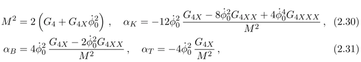
To get a non zero αT, one needs a model that does not preserve the relation be-tween the intrinsic and the extrinsic curvatures in eq. (2.12). Since the extrinsic curvatures give terms in ˙γij2 while the intrinsic one gives (∂kγij)2, changing the relation between them brings a change in the speed of sound of tensors. This hap-pens for example for what is known as the quartic galileon [22], whose Lagrangian is L4= G4(X)(4)R− 2G4X(X) [ (□ϕ)2− (∇µ∇νϕ)(∇µ∇νϕ) ] . (2.28)
The covariant second derivatives of the scalar field introduce first derivatives for the metric through the Christoffel symbols, which modifies the kinetic terms for gravity and gives a non zero αT. In unitary gauge this Lagrangian reads
L4 = G4R + (2XG4X− G4)(K2− KijKij) , (2.29) so that the EFT coefficients are
M2 = 2 ( G4+ G4Xϕ˙20 ) , αK =−12 ˙ϕ20 G4X− 8 ˙ϕ20G4XX + 4 ˙ϕ40G4XXX M2 , (2.30) αB= 4 ˙ϕ20 G4X− 2 ˙ϕ20G4XX M2 , αT =−4 ˙ϕ 2 0 G4X M2 , (2.31)
I will not discuss here the case of αH, which parametrizes deviations from Horndeski theories, since the next chapter is specifically focused on theories beyond Horndeski. In particular, the effect of αH will be explored in Section 3.6.
The theoretical origin of the parameters αaof eq. (2.19) is summarized in the following Table
M2 αM αK αB αT αH
Normalization
of the Planck mass Kinetic term Kinetic braiding Modification of Theories Interpretation tensor rate of change for between tensor beyond
quadratic action the scalar gravity and scalar sound speed Horndeski
≡ Planck mass
Example GR f (R) [23] k-essence Cubic Galileon Quartic Galileon G3theories
(when constant) Brans-Dicke [24] [25] [21] [22] (see Chapter3)
Table 2.1: In the first row, the parameters αi introduced in eq. (2.19).
2.4
Stability and theoretical consistency
Even if the terms in eq. (2.19) passed the first condition of yielding second-order dynam-ics (which guarantees the absence of extra, ghost-like DOF), further restrictions need to be imposed on the EFT parameters. Indeed, before thinking about comparing the
predictions of a theory to observations, stringent constraints must be imposed in order for the theory to be stable. This is where using a parametrization at the level of the action and not of the EOM has a clear advantage, since these stability conditions can in principle be read off directly from the action. The idea can be simplified thusly: in the case of two scalar fields3 ψ1(t, ⃗x), ψ2(t, ⃗x) their quadratic Lagrangian is generically
of the form:
L = ξ ˙ψ12− c1∂iψ12+ ˙ψ22− c2∂iψ22+ Vint(ψ1, ψ2). (2.32)
In this illustrative case, the stability of the theory requires the coefficient ξ to be positive. When this is not the case, the field ψ1is called a ghost and in general violent instabilities
are present in the theory.
Let me give some intuition on why that is, by thinking of the Lagrangian as L = T− V , where T is the kinetic energy and V the potential one. If the two signs are not the same in T , kinetic energy can flow without limits from one field to the other without changing the total energy E = T + V , meaning that the ground state of the theory is not stable (see [26] for a discussion on classical and quantum ghosts).
On top of this, one needs to impose that the coefficients c1 and c2 (which represent the
squared sound speeds) are positive, to avoid gradient instabilities. These instabilities can be understood very easily from the EOM: when varying (2.32) with respect to ψ1
for example, one gets
¨ ψ1− c1∆ψ1 = 1 2 ∂Vint ∂ψ1 . (2.33)
If c1 is negative, this equation admits in Fourier space a solution ψ⃗k proportional to
e √
|c1|kt, which is divergent.
The analysis in the case of the action (2.19) is more involved, since tensor modes are present on top of the scalar. Moreover, other non dynamical variables are present (scalar and vector), so that at first glance the form of the quadratic action is not as simple as (2.32). If we parametrize the unitary gauge metric as before
N = 1 + δN , Ni= ∂iψ + NVi , hij = a2e2ζ(δij+ γij) , (2.34) with ∂iNVi = 0 and γii= ∂iγij = 0, only ζ and γij are dynamical4. Once the constraints are solved, the quadratic part of the action can be rewritten in terms of dynamical DOF only, in a manner very similar to eq. (2.32):
S = ∫ d4xM 2a3 2 { α (1 + αB)2 [ ˙ ζ2− c2s∂iζ 2 a2 ] + ˙γ 2 ij 4 − (1 + αT) ∂kγij2 4a2 + (∂iNjV + ∂jNiV)2 4a4 } . (2.35) I have used the following definitions
α ≡ αK+ 6α2B, (2.36)
3
I will not treat the case of one field, as it present less interests. In particular, one cannot have a ghost field in this case: the sign of the kinetic term does not matter when there is nothing to compare it to. Moreover, in cosmology, the scalar field is always coupled to gravity.
4In general, the spatial metric contains also a (non-dynamical) vectorial part, which can be set to
and c2s≡ 2 { 1 + αT −1 + αH 1 + αB ( 1 + αM − H˙ H2 ) − 1 H d dt ( 1 + αH 1 + αB )} , (2.37)
the latter being valid only in the absence of matter. The stability conditions discussed above can be stated as
M2 > 0 , αK+ 6α2B > 0 ,
c2T ≡ (1 + αT) > 0 , c2s > 0 ,
(2.38) which defines the tensor sound speed.
The presence of matter, both at the background and perturbative levels, slightly com-plicates the situation. In the case αH = 0, one finds
c2s = 2(1 + αB) 2 α { 1 1 + αB ( 1 + αM − ˙ H H2 ) − (1 + αT)− ˙ αB H(1 + αB)2 } − ρm+ pm α M2H2 , (2.39) while the speed of sound for matter and tensors are unchanged. In the case αH ̸= 0, which will be treated in more details in Chapter 3, both the sound speed of matter and the extra scalar field are affected.
Of course, the conditions (2.38) can be translated into conditions on parameters of models, using for example Section 2.3. However, the advantage of the EFT of DE is that those conditions are really imposed on deviations from ΛCDM, not just on a specific model. It might well be that the regions of the parameter space they allow are not fully explored by any of the known theories (which lead us to the theories beyond Horndeski of Chapter 3). As we will see, the same kind of reasoning applies to the comparison with observations.
2.5
Evolution of cosmological perturbations
In this section I will discuss the effects of the deviations from ΛCDM on the evolution of perturbations, in the vector, tensor and scalar sectors, the latter being the richest–and most complicated–in term of phenomenology. The matter sector will be parametrized by its total stress energy tensor, decomposed at linear order as
T00 ≡ −(ρm+ δρm) , (2.40) T0i ≡ ∂iqm+ ( T0i)T ≡ (ρm+ pm)∂ivm+ ( T0i)V , (2.41) Tij ≡ (pm+ δpm)δji+ ( ∂i∂j− 1 3δ i j∂2 ) σm+ ( ∂iCj+ ∂jCi )V +(Tij)T T , (2.42) where δρm and δpm are the energy density and pressure perturbations, qm and vm are
respectively the 3-momentum and the 3-velocity potentials; σm is the anisotropic stress
potential. (T0i)V is the transverse part of the matter energy flux, (∂iCj + ∂jCi )V
and (Tij)T T are respectively the transverse and the transverse-traceless parts of the spatial matter stress tensor.
2.5.1 Vector sector
As we have seen from eq. (2.35), the vector sector is the simplest one as it does not contain propagating DOF. However, the presence of a time varying Planck mass, char-acterized by αM ̸= 0 still affects the perturbations. Indeed, when considering the full action supplemented by matter, the vector equation reads:
1 2∇ 2NV i = a2 M2 ( T0i)V . (2.43)
For a perfect fluid where CiV = 0, the conservation of the matter stress-energy tensor implies that (T0i)T ∝ 1/a3 [27]. Thus, the metric vector perturbations scale as
NVi ∝ 1 aM2 =
1
a1+αM , (2.44)
where the last equality holds for a constant αM. It is therefore interesting to see that the evolution of the vector sector only depends on a single parameter.
Since they typically decay, vector modes are very difficult to observe. This very fact already signals that αM cannot be too negative, i.e. the Planck mass cannot have been growing too strongly in time, otherwise they would not necessarily be negligible today. If vectors mode were to be detected, this would allow to constrain αM without having to treat the other parameters.
2.5.2 Tensor sector
The tensor sector, slightly more complicated, leads to the evolution equation ¨ γij + H(3 + αM) ˙γij − (1 + αT)∇ 2 a2 γij = 2 M2 (Tij) T T . (2.45)
Thus, even for a perfect fluid where the anisotropic stress is zero, the propagation of tensor modes is affected both by an additional friction term proportional to αM, as well as a different speed of propagation. In principle, the combined observation of vector and tensor modes could therefore provide constraints on αM and αT independently of each other and of the other αi.
2.5.3 Scalar sector
2.5.3.1 Obtaining the equations
In principle, five (non independent) scalar equations can be derived from the action (2.19). Four are the Einstein scalar equations (00, 0i, ii and ij traceless), where one needs to further introduce the scalar part of the traceless component of the spatial metric, χ
hij = a2(1 + 2ζ) [ δij + ( ∂i∂j − δij 3 ∂ 2 ) χ ] . (2.46)
Then, the action needs to be varied with respect to ζ, δN, ψ and χ, giving the four Einstein equations.
The fifth equation is the one for the scalar field ϕ. However, in unitary gauge this field is not explicit. One can still derive what would be the unitary gauge version of this equation (that will depend only on metric quantities) by imposing the invariance under time reparametrization of the action. Indeed, by definition of the unitary gauge,
δS[ϕ, gµν] δϕ(x) ϕ=t = δSu.g.[t, gµν] δt , (2.47)
where the time derivative is understood as a partial one (that is to say, not taking into account the time dependence of the metric).
For a general infinitesimal diffeomorphism xµ→ xµ+ ξµ, the metric changes as δgµν =
∇µξν +∇νξµ. Therefore, δSu.g.= ∫ d4x δSu.g. δgµν(x) (∇µξν(x) +∇νξµ(x)) + δSu.g. δt ξ 0 = 0 . (2.48)
After integrating by parts and combining this with eq. (2.47), one obtains that the equa-tion of the scalar field in unitary gauge is simply the zero component of the divergence of Einstein’s equations5, δS[ϕ, gµν] δϕ(x) ϕ=t = δSu.g. δt = 2g 0ν∇ µ δSu.g. δgµν = 0 , (2.49)
where the last equality holds when Einstein’s equations δSu.g.
δgµν = 0 are inforced. Hence,
this yields the fifth scalar equation, which is not independent from the others.
These five equations are for the scalar variables of the metric, namely ζ, δN, ψ and χ. To describe scalar perturbations and their physics, the Newtonian gauge is more adapted than the unitary gauge. In order to go from one to the other, a time diffeomorphism is performed
t→ t + π(t, ⃗x) , (2.50) where π describes the fluctuations of the scalar field
ϕ = t + π . (2.51)
In Newtonian gauge the scalar part of the metric is parametrized as
ds2 =−(1 + 2Φ)dt2+ a2(t)(1− 2Ψ)δijdxidxj . (2.52) One can relate the metric perturbations in unitary gauge defined in eq. (2.34) to he metric perturbations Φ and Ψ, as well as the scalar fluctuation π by6
δN = Φ− ˙π , ζ =−Ψ + Hπ , ψ = a−2π , χ = 0 . (2.53) Then, the five equations can be put in the following form (in Fourier space):
5
Since we assumed the presence of a Jordan frame, where matter is minimally coupled, its stress energy tensor is conserved independently.
6More precisely, to remove also the variable χ one needs a spatial diffeomorphism xi→ xi+ ∂ iβ,.
• The Hamiltonian constraint ((00) component of Einstein’s equation) is 6(1 + αB)H ˙Ψ + (6− αK+ 12αB)H2Φ + 2(1 + αH) k2 a2Ψ + (αK− 6αB) H 2˙π + 6 [ (1 + αB) ˙H + ρm+ pm 2M2 + 1 3 k2 a2(αH − αB) ] Hπ =−δρm M2 , (2.54)
• The momentum constraint ((0i) components of Einstein’s equation) reads
2 ˙Ψ + 2(1 + αB)HΦ− 2HαB˙π + ( 2 ˙H + ρm+ pm M2 ) π =−(ρm+ pm)vm M2 . (2.55)
• The traceless part of the ij components of Einstein’s equation gives
(1 + αH)Φ− (1 + αT)Ψ + (αM − αT)Hπ− αH˙π =−
σm
M2 , (2.56)
• The trace of the same components gives, using the equation above,
2 ¨Ψ + 2(3 + αM)H ˙Ψ + 2(1 + αB)H ˙Φ + 2 [ ˙ H−ρm+ pm 2M2 + (αBH)· + (3 + αM)(1 + αB)H 2 ] Φ − 2HαB¨π + 2 [ ˙ H + ρm+ pm 2M2 − (αBH)·− (3 + αM)αBH 2 ] ˙π + 2 [ (3 + αM)H ˙H + ˙ pm 2M2 + ¨H ] π = 1 M2 ( δpm− 2 3 k2 a2σm ) . (2.57)
• Finally, the evolution equation for π reads H2αKπ +¨ {[ H2(3 + αM) + ˙H ] αK+ (HαK)· } H ˙π + 6 {( ˙ H + ρm+ pm 2M2 ) ˙ H + ˙HαB [ H2(3 + αM) + ˙H ] + H( ˙HαB)· } π− 2k 2 a2Hπ˙ − 2k2 a2 { ρm+ pm 2M2 + H 2[1 + α B(1 + αM) + αT − (1 + αH)(1 + αM)] + (H(αB− αH))· } π + 6HαBΨ + H¨ 2(6αB− αK) ˙Φ + 6 [ ˙ H +ρm+ pm 2M2 + H 2α B(3 + αM) + (αBH)· ] ˙ Ψ + [ 6 ( ˙ H +ρm+ pm 2M2 ) + H2(6αB− αK)(3 + αM) + 2(9αB− αK) ˙H + H(6 ˙αB− ˙αK) ] HΦ + 2k 2 a2 { αHΨ + [H(αM˙ + αH(1 + αM)− αT)− ˙αH] Ψ + (αH− αB)HΦ } = 0 . (2.58) These equations are much more involved than in the two other sectors and as such are not readily useful. Nevertheless, one has to remember that there is only one propagating degree of freedom, which means that 4 of these equations are just constraints. Therefore, the five equations can be combined into a single equation for a single variable, e.g.
¨ Ψ +β1β2+ β3α 2 Bk˜2 β1+ α2B˜k2 H ˙Ψ + β1β4+ β1β5 ˜ k2+ c2 sα2B˜k4 β1+ α2B˜k2 H2Ψ = − 1 2M2 [ β1β6+ β7α2B˜k2 β1+ α2Bk˜2 δρm+ β1β8+ β9α2Bk˜2 β1+ α2B˜k2 H(ρm+ pm)vm− αK α δpm ] , (2.59)
where ˜k ≡ k/(aH), α is defined in eq. (2.36) and for simplicity, I have assumed that the anistropic stress of matter is zero. The βi are functions of the coefficients αj, whose–rather cumbersome–expressions are given in Appendix C of ArticleGin the case
αH = 0. Although this equation is enough to describe the dynamics of the scalar sector, it is useful to have the relation between the two metric potentials Φ and Ψ to connect with observations (in particular lensing). This relation takes the form
α2B˜k2 [ Φ− Ψ ( 1 + αT + αT − αM αB )] + β1 [ Φ− Ψ(1 + αT) ( 1 + ααT − αM 2β1 )] = αT − αM 2H2M2 { αB [δρm− 3H(ρm+ pm)vm] + HM2α ˙Ψ + H αK 2 (ρm+ pm)vm } . (2.60)
To complete the system of equations, one needs to provide the evolution equations for the matter sector. Since it is assumed to be minimally coupled, these equations come from the conservation of the stress energy tensor. At linear order in the perturbations, treating one species of matter only for simplicity, they read
˙δm− 3H(wmδm− δpm)− (1 + wm) ( k2 a2vm+ 3 ˙Ψ ) = 0 , (2.61) ˙vm− [ 3Hwm− ˙ wm 1 + wm ] vm+ δpm 1 + wm + Φ = 0 , (2.62)
with the definitions
wm≡ pm ρm , δm≡ δρm ρm , (2.63)
where wmis the usual equation of state parameter and δmthe density contrast. Note that
in general, when the fluid is not at rest, the relation between the pressure perturbation and the density contrast involves more than just the speed of sound (see for example [28]) which is why I kept explicitly δpm in these equations.
2.5.3.2 Interpretation
The system of equations (2.59)–(2.62) is complete (provided δpm and wm are specified)
and can in principle be solved to get the evolution of the matter perturbations and gravitational potentials. To do so without approximations would require a numerical implementation. However, the physics can be discussed analytically in specific cases, that give an idea of the effects expected. In particular, I will focus on the role played by
kinetic braiding. Indeed, one can see appearing in eq. (2.59) a new scale when αB ̸= 0:
kB =
aHβ1/21 αB
, (2.64)
which has been called braiding scale [19]. We shall explore two examples that show it is associated with noticeable modifications of gravity.
• αB = 0:
It can be seen as the extreme limit where kB → ∞, meaning that all modes are outside of the braiding length, k≪ kB. In this case most of the scale dependences go away. We are left with the simpler expression
¨ Ψ + (4 + 2αM + 3Υ) H ˙Ψ + ( β4H2+ c2s k2 a2 ) Ψ = − 1 2M2 { c2s[δρm− 3H(ρm+ pm)vm] + (αM − αT + 3Υ)H(ρm+ pm)vm− δpm } , (2.65) where Υ is defined in Appendix C of Article G. Although both αM and αT can be nonzero here, the form of this equation is very similar to that obtained in the standard k-essence case [25]. One recovers in the quasistatic limit (i.e. by neglecting time derivatives and taking k≫ aH/cs)
−k2 a2Ψ = 1 2M2δρm, Φ = (1 + αT) [ 1 + αKαT − αM 2β1 ] Ψ . (2.66)
This means that no scale dependence is introduced in the effective Newton constant defined as
−k2
a2Φ≡ 4πGeffδρm. (2.67)
As we will see, this no longer necessarily holds when αB ̸= 0.
• α2
B ≫ αK:
This case corresponds to having most of the kinetic energy of the scalar field coming from kinetic braiding. Indeed, one can see in this case that the kinetic energy (the term in ˙ζ2 in eq. (2.35)) is dominated by the contribution of α
B. For simplicity we consider only the case αT = 0. Moreover, to avoid gradient instabilities the following relation is required (see eq. (2.39))
αB≲ O(αM) . (2.68)
However, no restrictions are imposed on αM, whose value can affect the braiding scale. Indeed, when α2B ≫ αK, this is given by
k2B
a2 ≃ 3(H 2α
which can be inside the Hubble horizon. In this case, considering modes with k≫ kB, eq. (2.59) simplifies to ¨ Ψ + (3 + αM)H ˙Ψ + ( k2Bβ5 a2 + c 2 s k2 a2 ) Ψ≃ − 1 2M2 ( k2Bβ6 k2 + c 2 s+ 1 3− αM 3αB ) δρm, (2.70) where we have neglected relativistic terms on the right hand side of (2.59). If the ratio β5/c2s is larger than one, the scale dependence cannot be neglected even in the case k≫ kB. Therefore, a non vanishing αB, or the fact that kB <∞, brings a transition scale in the effective Newton constant7, which is a strong signal that gravity is modified.
Another interpretation would be that dark energy clusters: one can write Einstein equations as
Gµν = T µν m + TDµν
M2 , (2.71)
which defines effective fluid variables for dark energy/modified gravity. Thus, for subhorizon scales, the Poisson equation has the form
−k2 a2Φ =
1
M2 (δρm+ δρD) . (2.72)
For a cosmological constant, there are no perturbation in the dark energy fluid,
δρD = 0, and the standard behavior is recovered. However, as soon as dark energy clusters, i.e. δρD ∼ O(δρm), the relation between the gravitational potential
and matter is no longer as simple, leading to a different (and potentially scale dependent) effective Newton constant.
The equations (2.59) and (2.60) can be seen as the generalization to arbitrary scales of the usual parametrization in term of Geff (defined in eq. (2.67)) and the slip parameter
γ ≡ Ψ
Φ, (2.73)
that are employed in the quasistatic limit. However, if this limit is clearly defined in GR where it means focusing on subhorizon scales k≫ aH, its definition in the presence of an extra scalar field is more ambiguous. Indeed, in general, new scales (see [29] for a general discussion concerning new scales in modified gravity) and time dependences appear and its not always clear how this limit would translate, although in general it is expected to hold well inside the sound horizon of the scalar perturbations, kcs ≫ aH. To alleviate this uncertainty, one can look at what is called the extreme quasistatic limit [19] corresponding to wavenumber k much bigger than any scale in the problem, i.e. taking k→ ∞ in eqs. (2.59)–(2.60). This yields the following expressions
8πGeff = α c2s(1 + αT) + 2 [αB(1 + αT) + αT − αM]2 α c2 s M−2, (2.74) γ = α c 2 s+ 2αB[αB(1 + αT) + αT − αM] α c2 s(1 + αT) + 2 [αB(1 + αT) + αT − αM]2 , (2.75)
7Although the standard relation defining G
eff involves Φ and not Ψ, it easy to convince oneself that
where I have expressed both quantities directly in terms of the functions αa(recall that
α = αK+ 6α2B and αH is here set to zero). These two quantities are observable since the first affects directly the growth of structures and therefore affects the power spectrum of the large scale structure. The second is related to the gravitational potential felt by photon, Φ + Ψ, and thus can be probed in weak lensing experiments (see for example [30]).
In this Section, I have shown that by looking at the evolution of cosmological pertur-bations, one can relate the parametrization of the action in eq. (2.19) to observable quantities. The simplest cases from the theoretical side are the vector and tensor sec-tors. They only depend on the time variation of the Planck mass, αM, and on the deviation from unity of the tensor sound speed, αT. However, these sectors are precisely the fields of observations where the signals are the weakest.
The more experimentally accessible scalar sector corresponds to the most complicated domain, where all five functions αi play a role. Although their effects are understood from a theoretical point of view (see Table 2.1), they appear in a non trivial way when going to observable quantities such as the growth of structures or weak lensing. This can be seen analytically in the quasistatic limit with the modifications of the way matter sources the gravitational potential (through Geff) or the way the two potentials are
related to each other (through γ). This is why, to break the degeneracies that remain, one may need to go beyond the quasistatic limit, starting for example from eq. (2.59). One idea would be to solve perturbatively eqs. (2.59)–(2.62) around k → ∞ without necessarily making assumptions on the time derivatives. This would be a way to see the range of validity of the quasistatic approximation (see also [31]). We have actually started looking into this, but taking care of the time dependence is rather subtle and requires more work.
2.6
Conclusions
In this chapter, I presented a method called the Effective Field Theory for Dark Energy, that allows to explore the vast landscape beyond the standard model of cosmology, ΛCDM. It is based on the parametrization of an action, describing scalar-tensor theories in a very broad sense. I used the preferred time foliation that the scalar field offers, along with its 3+1 geometry, to construct a very generic Lagrangian that describes linear perturbations with second-order dynamics. This Lagrangian depends only on five functions of time, provided the expansion of the Universe and its matter content are known.
This has many advantages, both theoretically and observationally. The stability condi-tions that one needs to impose for a theory to be sensible can be easily read from this action. Moreover, this reduces to a single channel of analysis the comparison to exper-iments. The straigthforward links that we developped between wide classes of models and the parameters make it particularly convenient to use, since constraints on the five parameters easily translate to constraints on models.
However, this point of view is somewhat limiting the potential of this approach. The action (2.19) explores domains beyond the models currently known, potentially leading to new models, as we shall see in the next chapter. Indeed, it is solely based on the fact
that in general, the background solution of an additional field in a cosmological setting explictly breaks time reparametrization invariance. This opens the possibility of new terms in the action beside the standard Ricci scalar. It really is deviations from ΛCDM +GR that are captured by this formalism.
Because of its minimal number of parameters, the EFT of DE has started to be used by the community. It first started with people developing codes, in particular [32], that is based on the popular CMB code CAMB [33] and others doing forecasts for galaxy surveys [34]. Now, the parametrization, conveniently optimized by [19], is being used in the analysis of the Planck collaboration [35]. Hopefully, future surveys such as EUCLID [2] and LSST [3] will also use it, and the constraints on the αa will improve.
From a theoretical point of view, there is still work to be done. As I mentioned above, there is a yet untamed wealth of information contained in eq. (2.59), which includes for example relativistic effects that become important when looking at increasingly large surveys. It would be interesting to see how much of this information can be extracted using numerical solutions, or analytical method generalizing the quasistatic limit. Another point I have been working on recently consists of extending this formalism to the case of where the Weak Equivalence Principle (WEP) is violated, i.e. species couple to different metrics. This has been studied for ΛCDM under the name of interacting dark energy (see for example [36–39]). The idea is to investigate the interplay between these two properties, namely modifications of gravity and violation of the WEP. In particular, one can generalize the stability conditions (2.38), as well as the evolution equations (2.59)–(2.62) to include the different couplings of the matter fields, to look at the effect on the power spectrum and weak leasing.
Beyond Horndeski
Although using parametrizations such as the EFT of DE (for other examples, see [40,41]) proves useful when testing our understanding of cosmology, finding a more complete de-scription through a specific model provides advantages. For example, it allows to go beyond the linear approximation, which is necessary when looking at smaller scales, where it breaks down. A very important step in this endeavour was the work of Horn-deski [4] and its rediscovery [22, 42]. What are now known as Horndeski theories, or generalized galileons, are the most general Lorentz invariant scalar-tensor theories lead-ing to second-order equations of motion, both for the scalar and for the tensors. This property guarantees that they are well behaved and free of ghosts. The fondness for these theories comes from the standard lore that theories ruled by EOM with more than two derivatives should be automatically discarded because they suffer from instabilities, according to Ostrogradski’s theorem. However, this reasoning is too hasty. Indeed, in order for this statement to be correct, the theory needs to be non degenerate, in a sense that I will make clear later.
In this chapter, I will describe scalar-tensor theories that are not contained in Horn-deski’s. As a consequence, their EOM contain terms with three derivatives, but I will show that the theories are still “healthy”, meaning devoid of Ostrogradski’s instability. First, I will spend some time on what Horndeski theories are, before moving to these new theories, that we dubbed G3 for “Generalized Generalized Galileons”. Finally, I will use the formalism of Chapter 2 to explore the novel phenomenology that appears when going beyond Horndeksi.
3.1
Horndeski theories
As I have said before, the easiest way to modify ΛCDM is to introduce a scalar field. The goal is therefore to write a Lagrangian for this scalar field
L(ϕ, ϕα ≡ ∇αϕ, ϕβγ ≡ ∇β∇γϕ, gµν, . . .) . (3.1)
Usually, when writing such Lagrangians, only first derivatives of the scalar field are involved. However, one can be more general and include terms such as □ϕ ≡ gµνϕµν. They are slightly more delicate, as they can lead to extra, unstable DOF. A sufficient
condition to avoid this is to require that the EOM derived from the Lagrangian are at most second-order in derivative. Before turning to the case of a general metric gµν it is instructive to focus on the Minkowski limit, where the only dynamical DOF is the scalar. The key ingredient are the so-called galileons Lagrangians of [43]:
Lgal,12 = X , (3.2) Lgal,13 = X□ϕ − ϕµϕµνϕν , (3.3) Lgal,14 = X[(□ϕ)2− ϕµνϕµν ] − 2(ϕµϕνϕ µν□ϕ − ϕµϕµνϕλϕλν) , (3.4) Lgal,15 = X[(□ϕ)3− 3(□ϕ)ϕµνϕµν+ 2ϕµνϕνρϕµρ ] (3.5) − 3[(□ϕ)2ϕµϕµνϕν − 2□ϕϕµϕµνϕνρϕρ− ϕµνϕµνϕρϕρλϕλ+ 2ϕµϕµνϕνρϕρλϕλ ] ,
which are can be generalized to
LMink2 = A2(ϕ, X) , (3.6) LMink3 = A3(ϕ, X)□ϕ , (3.7) LMink4 = A4(ϕ, X) [ (□ϕ)2− ϕµνϕµν ] , (3.8) LMink5 = A5(ϕ, X) [ (□ϕ)3− 3(□ϕ)ϕµνϕµν+ 2ϕµνϕνρϕµρ ] , (3.9)
where here ϕµν = ∂µ∂νϕ since this is in flat space. For the choice of functions Aa∝ X one recover the previous expressions up to total derivatives.
The action S = ∫ d4x∑aLMinka constitutes the most general action for a scalar in flat space that leads to second-order EOM. What is essential in order to avoid higher derivatives is the antisymmetric structure that appears, in particular in the quartic (3.8) and quintic (3.9) galileons. Note that the same sort of structure appears in ghost-free massive gravity [44, 45] when focusing on the scalar mode (taking the so-called decoupling limit).
If we now want to write a covariant version of the most general action leading to second-order EOM in curved spacetime, the allowed Lagrangians can be decomposed into four classes LH2 [G2]≡ G2(ϕ, X) , (3.10) LH3 [G3]≡ G3(ϕ, X)□ϕ , (3.11) LH4 [G4]≡ G4(ϕ, X)(4)R− 2G4X(ϕ, X) [ (□ϕ)2− ϕµνϕµν ] , (3.12) LH5 [G5]≡ G5(ϕ, X)(4)Gµνϕµν+ 1 3G5X(ϕ, X) [ (□ϕ)3− 3 □ϕ ϕµνϕµν+ 2 ϕµνϕνρϕρµ ] . (3.13) The first type (3.10) corresponds to quintessence and k-essence, while the second (3.11) corresponds to the kinetic gravity braiding Lagrangian (2.26).
The third Lagrangian (3.12) contains the Einstein Hilbert action (2.12), for G4 =
MPl2/2. When G4X ̸= 0 the second piece has the structure inherited from the
quar-tic galileon (3.8). However, when the metric is dynamical and the partial derivatives are replaced by covariant ones, a non minimal coupling term, G4(ϕ, X)(4)R, is needed
quintic generalized galileon, is the extension of (3.12) to more fields ϕ. The list stops there because any Lagrangian with more fields satisfying Horndeski’s conditions would be a total derivative.
In the following section, I am going to argue that one can in fact write a more general action that is still stable, even though it possesses terms with more than two derivatives in the EOM.
3.2
General considerations on higher order derivatives
The desire for second-order EOM stems from Ostrogradski’s theorem, which can be stated as following: imagine the position q(t) of a particle is described by a Lagrangian
L(q, ˙q, ¨q) . (3.14) Note that, usually, the Lagrangian does not depend on the second derivative of the position. In this peculiar case, one can define the conjugate momenta to these variable as P1 ≡ ∂L ∂ ˙q − d dt ∂L ∂ ¨q , P2 ≡ ∂L ∂ ¨q . (3.15)
Ostrogradski’s theorem states (see for example [46]) that if the system is non-degenerate, i.e. if one can express the variable ˙q and ¨q as functions of P1 and P2, the system will
suffer from ghost instabilities as discussed in Section 2.4. In this simple case, the non degeneracy conditions translates simply to the invertibility of the 2x2 matrix
∂L ∂q(i)
∂L
∂q(j), (3.16)
where q(j) denotes the j-th derivative of q w.r.t. time. It is easy to convince oneself that when this is the case, the EOM contains terms with more than two time derivatives. Indeed, even though Ostrogradski’s proof is formulated at the level of the action, its consequences can be directly seen in the EOM. Let’s take the case of single DOF, ψ(t), whose EOM contains three time derivatives1. This means that, in order to evolve ψ from an initial state, one needs three conditions: the usual “position” ψ(t0) and “velocity”
˙
ψ(t0) but also the “acceleration” ¨ψ(t0). This goes against the idea that a DOF is given
by the couple position-momentum. It signifies the presence of an extra DOF, which, according to Ostrogradski, is a ghost (in the sense of eq. (2.32) with ξ < 0).
At the root of the proof is a notion of non degeneracy. This is not apparent in the case of one field since as soon as there is a higher derivative in the EOM, one must specify more initial conditions. However, when considering an action for more than one field, the non degeneracy conditions are not always this trivial: one can have the coefficient in front of higher derivative non zero but still have a degenerate system. A simple example
1
Note that the case of three derivatives is somewhat particular, since only one additional initial condition in needed, instead of the two associated with a full DOF. Moreover, it is not possible to construct a Lagrangian for a single field ψ that gives odd number of time derivatives. However, it can happen when more than one field are present and constitutes thus a case worth mentioning.
is the following set of equations ... ψ +...ϕ + H1ψ + H¨ 23ϕ = 0 , ¨ ψ + ¨ϕ− H3ϕ = 0 ,˙ (3.17)
where the Hi are arbitrary constants. Naively, one could think this would require three initial conditions for ψ and ϕ, for a total of six, and the apparition of a third DOF. How-ever, by plugging the second equation in the first, one can see the system is degenerate, since it is equivalent to
H3ϕ + H¨ 1ψ + H¨ 23ϕ = 0 ,
¨
ψ + ¨ϕ− H3ϕ = 0 ,˙
(3.18)
which is a standard second-order system describing two DOF.
The case of Lorentz invariant scalar-tensor theories is even more involved. Indeed, be-cause of the gauge freedom, the system is degenerate: we saw for example in Section2.4
that the lapse N and the shift Ni yielded constraint equations. This explains the fact that even GR, which a priori has ten DOF (the ten components of the metric), propa-gates only two.
In the case of eqs. (3.4) and (3.5) (as well as the other quartic (3.12) and quintic (3.13) Lagrangians), the degeneracy is increased by the specific antisymmetric structure of the Lagrangians: in particular, one can see that because of this structure, ∂2La
∂ ¨ϕ2 = 0. Of
course, as I said above, the degeneracy condition is really on the full matrix (3.16), but intuitively this is a sign that the theory is more degenerate.
It is exactly this degeneracy that would render the proof of Ostrogradski inapplicable in the Lagrangians of Horndeski, even before studying the EOM. Therefore, this realization gives hope that one can construct theories that are more general than Horndeski with-out introducing ghost DOF by considering Lagrangians that are deignerate enough. It should be noted that this is not a miracle recipe that would get rid of every ghost. The larger the number of derivatives, the more degenerate the theory needs to be, making it harder and harder to conceive one.
3.3
Generalized Generalized Galileons G
3Before introducing G3 theories, let me make a general remark here. When taking the flat space limit of any scalar-tensor theory, the possibility of non trivial degeneracy disappears since only the scalar remains. There, the number of possibilities is limited to the Lagrangians (3.6)–(3.9). This is why a necessary condition for any scalar-tensor theory to be ghost free is to reduce to these Lagrangians when gµν → ηµν2.
With this idea in mind, in [GLPV2,GLPV3] we studied the following Lagrangians
L4= LH4 [B4(ϕ, X)] + F4(ϕ, X)Lgal,14 , (3.19)
L5= LH5 [B5(ϕ, X)] + F5(ϕ, X)Lgal,15 , (3.20)
2
When this is not the case, the theory might be ghost free around specific background, but the property might not be Lorentz invariant.
where Lgal,14 and Lgal,15 the Lagrangians from eqs. (3.4) and (3.5) with the replacement
ηµν → gµν, ∂µ→ ∇µ. (3.21)
Under this form it is easy to see that the Horndeski case corresponds to F4 = F5 = 0.
However, when these functions are not zero, the EOM contain terms with three deriva-tives. More precisely, the metric equations contain three derivatives of the scalar and the scalar field equation contains three derivative of the metric. This means that when going to flat space, the scalar field recovers its second-order EOM, which is expected since it flat space these Lagrangians reduce to eq. (3.8)–(3.9) (up to total derivatives, see Article F).
This is not how we first discovered these Lagrangians. The first hint we had was when looking at the EFT of DE and realizing that, at linear order, one could be more general than Horndeski theories: we had an additional parameter αH in eq. (2.19) that accounted for a deviation from Horndeski, while keeping the right number of DOF. We then built a non linear theory that respected this property. Therefore, when we first wrote it, it was in the context of the EFT of DE and as such it was in unitary gauge. Using eqs. (2.4) and (2.13), the Lagrangians (3.19) and (3.20) can be recast into:
L4 ≡ A4(ϕ, X) ( K2− KµνKµν ) + B4(ϕ, X)R , L5 ≡ A5(ϕ, X) ( K3− 3KKµνKµν+ 2KµνKνρKµρ ) + B5(ϕ, X)Kµν ( Rµν− 1 2hµνR ) , (3.22) where A4≡ −B4+ 2XB4X− X2F4, A5≡ − XB5X 3 + (−X) 5/2F 5. (3.23)
This yields the expression of the Horndeski Lagrangians in terms of 3+1 quantities in the case F4 = F5 = 0, which was first derived in [GLPV1]. On top of making the
connection with Chapter 2 easier, these expressions are going to allow us to prove that the theory has no extra DOF. In order to do so, we will specialize to the case where the scalar field is spacelike, so that we can go to unitary gauge.
One could rightfully argue that proving the soundness of the theory under this assump-tion does not guarantee it will hold on a different background. This is indeed true. However, it is a necessary condition and under this assumption one can actually say something quantitative about the number of DOF. Moreover, the fact that it also re-duces to galileons in Minkowski is a strong signal that the theory is safe around any background. I will give a purely Lorentz invariant proof in a following section, which relies on knowing a priori a transformation of the metric that maps subsets of G3 onto