Exploiting independence in a decentralised and incremental approach of diagnosis

HAL Id: inria-00110584

https://hal.inria.fr/inria-00110584

Submitted on 31 Oct 2006

HAL is a multi-disciplinary open access

archive for the deposit and dissemination of

sci-entific research documents, whether they are

pub-lished or not. The documents may come from

teaching and research institutions in France or

abroad, or from public or private research centers.

L’archive ouverte pluridisciplinaire HAL, est

destinée au dépôt et à la diffusion de documents

scientifiques de niveau recherche, publiés ou non,

émanant des établissements d’enseignement et de

recherche français ou étrangers, des laboratoires

publics ou privés.

Exploiting independence in a decentralised and

incremental approach of diagnosis

Alban Grastien, Marie-Odile Cordier

To cite this version:

Alban Grastien, Marie-Odile Cordier. Exploiting independence in a decentralised and incremental

approach of diagnosis. IJCAI 07, Jan 2007, Hyderabad. �inria-00110584�

Exploiting independence in a decentralised and incremental approach of diagnosis

Marie-Odile Cordier

University of Rennes1 / Irisa

Rennes – France

[email protected]

Alban Grastien

National ICT Australia

Canberra – Australia

[email protected]

Abstract

It is well-known that the size of the model is a bottleneck when using model-based approaches to diagnose complex systems. To answer this problem, decentralised/distributed approaches have been proposed. Another problem, which is far less considered, is the size of the diagnosis itself. How-ever, it can be huge enough, especially in the case of on-line monitoring and when dealing with un-certain observations. We define two independence properties (state and transition-independence) and show their relevance to get a tractable represen-tation of diagnosis in the context of both decen-tralised and incremental approaches. To illustrate the impact of these properties on the diagnosis size, experimental results on a toy example are given.

1

Introduction

We are concerned with the diagnosis of discrete-event sys-tems [Cassandras and Lafortune, 1999] where the system be-haviour is modeled by automata. This domain is very active since the seminal work by [Sampath et al., 1996]. Its aim is to find what happened to the system from existing observations. A classical formal way of representing the diagnosis prob-lem is to express it as the synchronised product of the system model automaton and an observation automaton. This formal definition hides the real problem which is to ensure an effi-cient computation of the diagnosis when both the system is complex and the observations possibly uncertain.

It is now well-known that the size of the system model is a bottleneck when using model-based approaches to di-agnose complex systems. To answer this problem, decen-tralised/distributed approaches have been proposed [Pencol´e and Cordier, 2005; Lamperti and Zanella, 2003; Benveniste

et al., 2005; Jiroveanu and Bo¨el, 2005]. Instead of being

ex-plicitly given, the system model is described through its com-ponent models in a decentralised way. The global diagnosis is computed by merging local diagnoses in order to take into account the synchronisation events which express the depen-dency relation which may exist between the components.

∗_{This work was mainly made when the author was Ph.D student}

at University of Rennes1/Irisa, Rennes, France.

A problem, which is far less considered, is the size of the diagnosis itself. However, it can also be a problem, es-pecially when dealing with a long-lasting flow of uncertain observations as remarked in [Lamperti and Zanella, 2003]. We define in this paper two independence properties

(state-independence and transition-(state-independence) and show that

they make it possible to get a decentralised representation of the diagnosis without any loss of information. When the di-agnosis is performed on a long-lasting temporal window, the transition independence property, which expresses the con-currence between subsystems, has little chance of being satis-fied. The idea then is to slice the diagnosis period into smaller periods and to compute the diagnosis in an incremental way. The problem which appears is that the slicing generally re-moves the state-independence property. The solution we fi-nally propose is to enrich the representation with an abstract description of the diagnosis trajectories and show that it al-lows us to keep the benefits of the transition-independence based decentralised representation.

After preliminaries in Section 2, two independence prop-erties (state and transition-independence) on automata are defined in Section 3. In Section 4, the decentralised ap-proach is proposed and the decisive role played by the

state-independence property in the diagnosis computation is

high-lighted. Then it is shown how to take advantage of the

transition-independence property to get an efficient

represen-tation of the diagnoses. The incremental compurepresen-tation and the use of an abstract representation is considered in Section 5. To illustrate the impact of our proposal on the diagnosis size, experimental results on a toy example are given in Section 6.

2

Preliminaries

We suppose in this paper that the behavioural models are de-scribed by automata. We thus begin by giving some defini-tions concerning automata (see [Cassandras and Lafortune, 1999]). Then, we recall the diagnosis definitions and state some hypotheses.

2.1

Automata, synchronisation and restriction

An automaton is a tuple (Q, E, T, I, F ) where Q is the set

of states, E the set of events, T the set of transitions(q, l, q′₎ with l ⊆ E, and I and F the sets of initial and final states.

A trajectory is a path in the automaton joining an initial state to a final state. The set of trajectories of an automaton

A is denoted Traj(A). In the following, we consider trim

automata. The trim operation transforms an automaton by removing the states that do not belong to any trajectory.

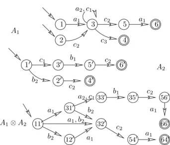
Example: Let us consider the first trim automaton in

Fig-ure 1. The initial states are represented by an arrow with no origin state, and the final states by a double circle. Then,

1{a−→ 31} {a2,c1} −→ 3{c3} −→ 4−→ 4 is a trajectory.∅ replacements 1 2 3 4 5 6 a1 c2 c2 c3 a1 a2, c1 A1 1′ 2′ 3′ 4′ 5′ ₆′ c1 b2 b1 c2 c2 A2 11′ 31′ 33′ ₃₅′ ₅₆′ 66′ 12′ 32′ 54′ ₆₄′ a1 a2, c1 b1 c2 a1 b2 b2 a1 c2 a1 a1, b2 A1⊗ A2

Figure 1: Two automata and their synchronisation The synchronisation operation on two automata A1 and

A2 builds the trim automaton where all the trajectories of both automata which cannot be synchronised according to the synchronisation events (i.e E1∩ E2) are removed. For-mally, given two automata A1 = (Q1, E1, T1, I1, F1) and

A2 = (Q2, E2, T2, I2, F2), the synchronisation of A1 and

A2, denoted A1⊗ A2, is the trim automaton A= Trim(A′)

with A′= (Q1×Q2, E1∪E2, T′, I1×I2, F1×F2) such that:

T′ = {((q1, q2), l, (q′1, q′2)) | ∃l1, l2 : (q1, l1, q1′) ∈ T1∧

(q2, l2, q2′) ∈ T2∧ (l1∩ (E1∩ E2) = l2∩ (E1 ∩ E2)) ∧

l= l1∪ l2}. When E1∩ E2 = ∅ (no synchronising events), the synchronisation results in the concurrent behavior of A1 and A2, often called the shuffle of A1and A2. The number of states of the shuffle is the product of the number of states of

A1and A2and no trajectory is removed.

Example: Figure 1 gives an example of synchronisation. The

synchronising events are the cievents.

The restriction operation of an automaton removes from I all the initial states which are not in the specified set of states. Due to the trim operation, all the states and transitions which are no longer accessible are removed from Q. Formally, given an automaton A= (Q, E, T, I, F ), the restriction of A by the

states of I′, denoted A[I′], is the automaton Trim(A′) with A′ _{= (Q, E, T, I ∩ I}′_{, F).}

2.2

Diagnosis

Let us recall now the definitions used in the domain of discrete-event systems diagnosis where the model of the

sys-tem is represented by an automaton. t0 corresponds to the starting time and tnto the ending time of diagnosis. More de-tails can be found for instance in [Pencol´e and Cordier, 2005].

Definition 1 (Model).

The model of the system, denoted Mod, is an automaton.

The model of the system describes its behaviour and the trajectories of Mod represent the evolutions of the system. The set of initial states IMod is the set of possible states at

t0. We suppose as usual that F Mod = QMod (all the states

of the system may be final). The set of observable events is denoted EMod_Obs ⊆ EMod.

Let us turn to observations which can be uncertain and are represented by an automaton, where the transition labels are observable events of EMod

Obs.

Definition 2 (Observation automaton).

The observation automaton, denoted Obs, is an automaton describing the observations possibly emitted by the system during the period[t0, tn].

The diagnosis of a discrete-event system can be seen as the computation of all the trajectories of the model that are con-sistent with the observations sent by the system during the period[t0, tn]. The automaton defined as the synchronisation of the model and the observations represents all these trajec-tories.

Definition 3 (Diagnosis).

The diagnosis, denoted ∆, is a trim automaton such that ∆ = Mod ⊗ Obs.

3

Independence properties

In this section, we present two independence properties that enable a decentralised (compact yet sufficient) representation of the diagnosis presented in the next section.

Let us first define the state-independence property which concerns the decomposition of an automaton A into two au-tomata A1and A2.

Definition 4 (Decomposition of A).

Two automata A1 and A2are said to be a decomposition of

an automaton A iff A= (A1⊗ A2)[I] where I are the initial

states of A.

Let A′ = A1⊗ A2. Note that we do not require that A=

A′, but that A′ is a super-automaton (i.e an automaton that contains all the trajectories of A and possibly more). The reason is that, when decomposing A into A1and A2, the links existing between the initial states of A1 and A2 can be lost. We thus have Q ⊆ Q′_{, I ⊆ I}′_{, and F ⊆ F}′ _{where A}′ ₌

(Q′, E′, T′, I′, F′) and A = (Q, E, T, I, F ).

The state-independence property is a property of a decom-position A1and A2which ensures that A= A′.

Definition 5 (State-independence decomposition wrt A).

Two automata A1and A2are said to be a state-independent decomposition wrt A iff A= A1⊗ A2.

Property 1: If A1 and A2 have both a unique initial state, and if they are a decomposition of A, then A1and A2are a state-independent decomposition wrt A.

Let us turn now to the transition-independence property which states that two (or more) automata do not have any transition labeled with common synchronisation events.

Definition 6 (Transition-independence).

A1 = (Q1, E1, T1, I1, F1) and A2 = (Q2, E2, T2, I2, F2)

are transition-independent (TI) iff every label l on a transition of T1or T2is such that l∩ (E1∩ E2) = ∅.

Two transition-independent automata are concurrent au-tomata and their synchronisation is equivalent to a shuffle op-eration (see Section 2). Moreover, we have :

Property 2: Let A1 and A2 be two transition-independent automata and state-independent automata wrt A. The states (resp. initial states, final states) of A correspond exactly to the Cartesian product of the states (resp. initial states, final states) of A1and A2.

4

Improving diagnosis representation in a

decentralised approach

In this section, we first highlight the role of state-independence property when computing diagnoses in a de-centralised way. We propose then an efficient diagnosis rep-resentation based on transition-independence property.

4.1

The decentralised approach and the role of

state-independence

The global model of a real-world system is too large to be explicitly built. To answer this problem, decentralised / distributed approaches have been proposed [Lamperti and Zanella, 2003; Pencol´e and Cordier, 2005; Benveniste et al., 2005; Jiroveanu and Bo¨el, 2005]. In this article, we consider the decentralised approach of [Pencol´e and Cordier, 2005].

The idea (see Figure 2) is to describe the system behaviour in a decomposed way by the set of its subsystems mod-els. The so-called decentralised model is thus dMod = {Mod1, . . . , Modn} where Modiis the behavioural model of the subsystem (possibly a component) si. The decentralised model is designed as a decomposition of the global model

Mod. It is generally assumed that the global model has a

unique initial state and that the subsystems models also have a unique initial state. They are thus a state-independent decom-position wrt Mod and the global model can thus be retrieved, if needed, by Mod= Mod1⊗ . . . ⊗ Modn.

The observations Obs can be decentralised as follows:

dObs = {Obs1, . . . , Obsn} such that Obsi contains the ob-servations from the subsystem si and such that: Obs =

Obs1⊗ . . . ⊗ Obsn.

Given the local subsystem model Modi and the local sub-system observations Obsi, it is possible to compute the lo-cal diagnosis ∆si = Modi ⊗ Obsi. These diagnoses

rep-resent the local subsystem behaviours that are consistent with the local observations. It was shown in [Pencol´e and Cordier, 2005] that the set of local diagnoses is a decom-position of ∆. As they all have a unique initial state, it

is also a state-independent decomposition of∆. It is then

possible to directly compute the global diagnosis of the sys-tem by synchronizing the subsyssys-tem diagnoses as follows:

∆ = ∆s1 ⊗ . . . ⊗ ∆sn. This synchronisation operation of

subsystem diagnoses is often also called a merging operation.

{Mod1, . . . , Modn} Mod {∆s1, . . . ,∆sn} ∆ local diagnosis synchronisation merging diagnosis

Figure 2: Principle of the decentralised diagnosis approach

It is clear that, rather than directly merging all the subsys-tems diagnoses together, it is possible to compute the global diagnosis by successive synchronisation operations. Let s1 and s2 be two disjoint subsystems (possibly being compo-nents) and let s12 = s1⊎ s2be the subsystem that contains exactly s1and s2. The subsystem diagnosis∆s12can be

com-puted as∆s12 = ∆s1 ⊗ ∆s2. The diagnosis of the system is

equivalently obtained by replacing∆s1 ⊗ ∆s2 by∆s12. We

have∆ = ∆s12⊗ ∆s3⊗ . . . ⊗ ∆sn.

Algorithm 1 computes the system diagnosis by starting from the component local diagnoses and merging them until ExitLoopCondition is satisfied. In this case, ExitLoopCondi-tion checks that all pairs of diagnoses have been merged.

Algorithm 1 Computing diagnoses in a decentralised way input: local diagnoses{∆s1, . . . ,∆sn}

d∆ = {∆s1, . . . ,∆sn} while¬ ExitLoopCondition do Choose∆s1,∆s2 ∈ d∆ s= s1⊎ s2 ∆s= ∆s1⊗ ∆s2 d∆ = (d∆ \ {∆s1,∆s2}) ∪ {∆s} end while return: d∆

4.2

An efficient diagnosis representation based on

transition-independence

The diagnosis∆ built with a decentralised approach is equal

to the synchronisation Mod⊗ Obs. It can be expected Obs

sufficiently contraints the behaviours of the system to signif-icantly reduce the size of the∆ compared to Mod. However ∆ can still be large, especially because merging concurrent

diagnoses corresponds to computing the shuffle of these diag-noses. It is why we propose to avoid these expensive shuffles by representing the system diagnosis as a set of transition-independent subsystem diagnoses.

Definition 7 (Decentralised diagnosis).

A decentralised diagnosis d∆ is a set of subsystem diagnoses {∆s1, . . . ,∆sk} such that ∆si is the diagnosis of the sub-system si, {s1, . . . , sk} is a partition of the system Γ, and

∀i, j ∈ {1, . . . , k}, i 6= j ⇒ ∆si and∆sj are transition-independent.

As seen before, a decentralised diagnosis d∆ = {∆s1, . . . ,∆sk} is a state-independent decomposition

of the global diagnosis. We get an economical represen-tation of the global diagnosis which can be computed, if needed, by synchronising all the subsystem diagnoses, by

∆ = ∆s1⊗ . . . ⊗ ∆sk, which, due to Property 2, corresponds

to a shuffle operation. Its final states can be obtained by a simple Cartesian product on the final states of all∆si (see

Property 2).

Algorithm 1 can be used to compute the decentralised di-agnosis from the local (component) diagnoses by changing ExitLoopCondition into ∀∆s1,∆s2 ∈ d∆, ∆s1 and ∆s2

are transition-independent. Until all pairs of diagnoses are independent, the algorithm chooses two transition-dependent diagnoses and merges them.

An important point to remark is the decisive role of the state-independence property of the decomposition which, combined to the transition-independence property, allows us to get an efficient representation of the system diagnosis. The state-independence property comes directly from the unique initial state property of the system and subsystems models.

5

Improving diagnosis representation in a

decentralised and incremental approach

In this section, we propose to build the diagnosis on succes-sive temporal windows, to benefit from the short duration independences. We then show that the state-independence is generally no longer satisfied, and present in the last part the abstraction operation that enables us to deal with state-dependent subsystems.

5.1

Incremental diagnosis

In the previous section, we assumed that the diagnosis was computed on a unique period. This means that the obser-vation automaton represents the obserobser-vations emitted dur-ing [t0, tn]. The problem of this approach is that long pe-riods transition-independent behaviours are infrequent, be-cause each component eventually interacts with most of its neighbours. Thus, all the local diagnoses will eventually be merged in a huge global diagnosis. For this reason, it can be interesting to divide the diagnosis period into temporal win-dows as presented in [Pencol´e and Cordier, 2005], to benefit from short duration independent behaviours.

Let us consider that the diagnosis∆i−1 of[t0, ti−1] was built and that the set of final states of this diagnosis is

F∆i−1. Given the observations Obs i

of the temporal window

[ti−1, ti], it is possible to compute the diagnosis of this tem-poral window by:∆i_{= (Mod}−_{⊗ Obs}i_)[Fi−1

∆ ] where Mod− is the system model Mod where all the states are considered as initial states. The trajectories consistent with the observa-tions for the period [t0, ti] (i.e the trajectories of ∆i if this automaton were built) can be retrieved by the concatenation of the trajectories from∆i−1and the trajectories of∆i. It can also be proved that the final states of∆iare the final states of

∆i_{. It is thus possible to incrementally add the observations} of[ti, ti+1] and compute the diagnosis.

5.2

Loss of the state-independence property

Our goal is to use a decentralised computation based on a de-centralised model and to represent the diagnosis of the tempo-ral windowWi _{= [t}

i−1, ti] by a set of transition-independent

subsystem diagnoses similar to Section 4. However, con-trary to Section 4, the unique initial state hypothesis can no longer be made and thus the state-independence decomposi-tion property can no longer be considered as satisfied.

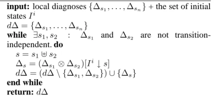
Let Ii_{be the set of initial states on the system for the} tem-poral windowWi_{. Given I}i_{, the set of initial states of a} sub-system s is called the projection of Ii_{on s and denoted I}i_{↓ s.} Let us remark that(Ii _{↓ s) × (I}i _{↓ s}′_{) ⊇ I}i _{↓ (s ⊎ s}′_). Al-gorithm 1 can be modified as presented in AlAl-gorithm 2 to compute a set d∆i_{of transition-independent subsystems} di-agnoses.

Algorithm 2 Computing transition-independent diagnoses in

case of non state-independence

input: local diagnoses{∆s1, . . . ,∆sn} + the set of initial

states Ii

d∆ = {∆s1, . . . ,∆sn}

while ∃s1, s2 : ∆s1 and ∆s2 are not

transition-independent. do s= s1⊎ s2 ∆s= (∆s1⊗ ∆s2)[I i_{↓ s]} d∆ = (d∆ \ {∆s1,∆s2}) ∪ {∆s} end while return: d∆

Let us now consider the transition-independent diagnoses of d∆i_{and more precisely their final states F}i

∆_sj. The prob-lem is that, due to the loss of the state-independence property,

Fi_{is only a subset of F} ∆i

s1× . . . × F∆isk. Let us illustrate the

problem on an example (Figure 3).

OO′ OF′ F O′ O F O′ _F′ f1 f2

Figure 3: Example of loss of information in a naive decen-tralised representation of the incremental diagnosis

Example Figure 3 deals with the diagnosis of two

compo-nents which can be either in a Ok state or a F aulty state. The figure presents a two-windows diagnosis, each in a box. During the first window (Figure 3, left), one of the two ponents failed but it is not possible to determine which com-ponent did. The initial states of each comcom-ponent at the be-ginning of the second window are obtained by projecting the final states of the first window and they are O and F for one component and O′ and F′ for the other one. Nothing hap-pened during the second window. Since the local diagnoses are transition-independent, the algorithm proposes the two lo-cal diagnoses (top and bottom in Figure 3, right) but it can be seen that the links between the initial states were lost during the projection. The decomposition of the global diagnosis is

not state-independent. We have F2 ⊂ {O, F } × {O′_{, F}′_}. To get the exact final states F2, one solution would be to syn-chronise the local diagnoses in conjunction with the restric-tion operarestric-tion on the set of final states of the first window as argument, which we want to avoid.

5.3

TI + abstract representation

To obtain the final states Fi _{we propose, instead of} merg-ing the state-dependent diagnoses of d∆i_{, to merge their} ab-stract representations, which is much more efficient. We thus propose to enrich the set of transition-independent diagnoses with the abstract representation of the state- and transition-independent diagnoses.

The information required relies on the initial and final states only. Thus, we define an abstraction that keeps only the in-formation that there exists a trajectory between an initial state and a final state.

Definition 8 (Abstraction).

Let A = (Q, E, T, I, F ) be a trim automaton. The

abstrac-tion of A, denoted Abst(A), is the (trim) automaton A′ ₌

(I ∪ F, {e}, T′, I, F) where T′ = {(q, {e}, q′) | ∃traj = q0

l1

−→ . . . ln

−→ qn∈ Traj(A) ∧ q0= q ∧ qn = q′}. The following two properties can be easily proved.

Property 3: Let A1 and A2 be two transition-independent automata. Then, Abst(A1) ⊗ Abst(A2) = Abst(A1⊗ A2).

Property 4: Let A1 and A2 be two transition-independent automata and let I be a set of states. Then, (Abst(A1) ⊗

Abst(A2))[I] = Abst((A1⊗ A2)[I]).

It is now possible to merge the abstract representations of the state-dependent, transition-independent diagnoses as pre-sented in Algorithm 3 until getting a set of state- and transi-tion independent diagnoses. This result is called the abstract

decentralised diagnosis, and denoted ad∆i_{. Given the} prop-erties 3 and 4, we have the following result:

Proposition 1.

The set of final states Fi is the set of final states of ad∆i_,

i.eΠ∆∈ad∆iF∆.

Let us define an extended decentralised diagnosis as follows :

Definition 9 (Extended decentralised diagnosis).

An extended decentralised diagnosis on Wi _{is a pair}

(d∆i_{, ad∆}i_{) such that}

• d∆i_{is the decentralised diagnosis of the system onW}i_,

• ad∆i is the abstract decentralised diagnosis on Wi_. The transition-independent diagnoses d∆i _{provide the set} of trajectories during the temporal windowWi _{and the} ab-stract representation of state- and transition-independent di-agnoses ad∆i_{provides the set of final states of the temporal} windowWi_{. It is thus a safe representation of the} diagno-sis on Wi_{. It can be used as shown in 5.1 to compute the} diagnosis on the whole period in an incremental way.

6

Experiments

We present the experimental results on a simplified case in-spired by a real application on telecommunication networks.

Algorithm 3 Computation of the abstract decentralised

diag-nosis ad∆i

input: local transition-independent diagnoses d∆i ₌

{∆i s1, . . . ,∆ i sk} + the set I i_{of initial states} ad∆i_{= {a∆}i sj | ∃∆ i sj ∈ d∆ i_{: a∆}i sj = Abst(∆ i sj)} while∃a∆i s1, a∆ i s2 ∈ ad∆ i_{such that a∆}i s1 and a∆ i s2 are

not state-independent wrt(a∆i s1⊗ a∆ i s2)[I i_{↓ s} 1⊎ s2] do s= s1⊎ s2 a∆i s= (a∆is1⊗ a∆ i s2)[I i_{↓ s]}

ad∆i _{= (ad∆}i_{\ {a∆}i s1, a∆ i s2}) ∪ {a∆ i s} end while return: ad∆

6.1

System

The system to diagnose is a network of14 interconnected

components as presented in Figure 4.

1 2 3 4 5 6 7 8 9 10 11 12 13 14

Figure 4: Topology of the network

Each component has the same behaviour: when a fault oc-curs, it reboots, sends a IRebooti observation and forces its neighbours to reboot by sending them a reboot! message. A component can also be asked to reboot by one of its neigh-bours. In this case, it enters into a waiting state W before rebooting and sends the IRebooti observation. In this state, it can be asked to reboot by another component (and sends then the IRebootiobservation). When the reboot is finished, the component sends the observation IAmBacki and reen-ters the state O.

The model is presented in Figure 5. The reboot! message indicates that reboot is sent to all the neighbours, and the

re-boot? message indicates that a neighbour has sent the reboot

message to the component. So, for example, on component1,

there are three transitions from state O to state W correspond-ing to a reboot? message received respectively from one of its three neighbours2, 3 and 14. They are respectively

la-beled by{reboot2→1, IReboot1}, {reboot3→1, IReboot1} and

{reboot14→1,IReboot1}. O W R F fault,reboot!,IReboot end,IAmBack reboot? end,IAmBack reboot?, IReboot start-reboot

reboot?, IReboot reboot?

Figure 5: Model of a component

ex-actly 4 × 14 states, while the global model would contain

nearly414_{≅250 000 000 states.}

6.2

Results

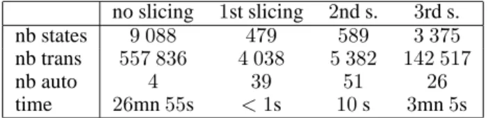
The algorithms were programmed in Java, and run on a Linux machine with a 1.73 GHz Intel processor. We deal with 45 observations. The experiments results are given Table 1.

The first experiment was made with a unique temporal win-dow as presented in section 4. The computation was more than 26 mn and produced4 automata, one of which contains 9 085 states and 557 836 transitions. It can be noted that

taking into account the transition-independence property of diagnoses in the decentralised representation is interesting as four independent subsystems are identified. It saves us from computing the shuffle for these subsystem diagnoses, which is certainly very beneficial. However, due to the length of the window, one of the automata is still very large.

Using the method described in section 5, the observations are now sliced into4 temporal windows. The diagnosis was

com-puted in less that1 second, producing 39 small automata. The

number of states (479) is 5% of the number of states used in

the previous automaton, and the number of transitions (4 038)

is less than1% of the transitions of the previous automaton.

It confirms that slicing observations is beneficial in that it in-creases the number of independent subsystems, and thus di-agnoses. no slicing 1st slicing 2nd s. 3rd s. nb states 9 088 479 589 3 375 nb trans 557 836 4 038 5 382 142 517 nb auto 4 39 51 26 time 26mn 55s <1s 10 s 3mn 5s

Table 1: Results of the experimentations

Let us stress now the importance of the slicing on the good results of the method. In a third experiment, the first temporal window of the previous experiment was sliced into two. The number of states of the diagnosis increased by about20%

and the number of transitions by30%. Moreover, the

com-putation time increased to 10 seconds. The reason is that you sometimes need to have enough observations on a sub-system to conclude that this subsub-system did not communicate with another subsystem. In a fourth experiment, two tem-poral windows of the first slicing are merged into a unique window. The corresponding computation time is then about3

minutes and the number of states and transitions exploded. It confirms that the slicing operation is a critical operation and that deciding what is the best slicing is an interesting area for further works.

7

Conclusion

In this paper, we consider the diagnosis of discrete-event sys-tems modeled by automata. To avoid the state-explosion problem that appears when dealing with large systems, we use a decentralised computation of the diagnosis. We show that the global diagnosis can be safely and economically rep-resented by the set of diagnoses of its transition-independent

subsystems. An important point is that this decentralised rep-resentation relies on the state-independency property.

When the period of observation is important, independent subsystems occur infrequently, since each component even-tually interacts with most of its neighbours. A solution is to slice the diagnosis period into temporal windows, in or-der to get, on these windows, transition-independent subsys-tems. The problem is that the state-independency property does not hold anymore. It is then impossible to get the ex-act final states, at least in an economical way. On the one hand, such a set of diagnoses for transition- but not state-independent subsystems gives us only a superset of the global diagnosis, which is not satisfying. On the other hand, com-puting the set of transition-independent and state-independent subsystem diagnoses would be too expensive.

We propose in this paper to keep the decentralised diag-nosis representation (a set of transition-independent subsys-tem diagnoses), and to add an abstract representation of both state- and transition-independent diagnoses, which produces the final states in an economic and efficient way. We show that we get a safe and efficient representation of the global diagnosis.

This work opens at least two interesting prospects. As can be seen in Algorithm 3, it is necessary to have an efficient way to check whether two abstract diagnoses are or are not state-independent, and we are currently working on this point. Another concern is about the slicing. As shown in section 6, a bad slicing can lead to a very little benefit. An interesting prospect would be to automatically find the best slicing to obtain a diagnosis represented as efficiently as possible.

Acknowledgements

A. Grastien is currently supported by National ICT Australia (NICTA) in the framework of the SuperCom project. NICTA is funded through the Australian Government’s Backing Australia’s

Ability initiative, in part through the Australian National Research

Council.

References

[Benveniste et al., 2005] A. Benveniste, S. Haar, E. Fabre, and Cl. Jard. Distributed monitoring of concurrent and asynchronous systems. Discrete Event Dynamic Systems, 15(1):33–84, 2005. [Cassandras and Lafortune, 1999] C. Cassandras and S. Lafortune.

Introduction to Discrete Event Systems. Kluwer Academic

Pub-lishers, 1999.

[Jiroveanu and Bo¨el, 2005] G. Jiroveanu and R. Bo¨el. Petri net model-based distributed diagnosis for large interacting systems. In Sixteenth International Workshop on Principles of Diagnosis

(DX-05), pages 25–30, 2005.

[Lamperti and Zanella, 2003] G. Lamperti and M. Zanella.

Diag-nosis of Active Systems. Kluwer Academic Publishers, 2003.

[Pencol´e and Cordier, 2005] Y. Pencol´e and M.-O. Cordier. A for-mal framework for the decentralised diagnosis of large scale dis-crete event systems and its application to telecommunication net-works. Artificial Intelligence Journal, 164(1-2):121–170, 2005. [Sampath et al., 1996] M. Sampath, R. Sengupta, S. Lafortune,

K. Sinnamohideen, and D. Teneketzis. Failure diagnosis using discrete-event models. Control Systems Technology, 4(2):105– 124, 1996.