Time-frequency tools of signal processing for EISCAT data analysis

HAL Id: hal-00329066

https://hal.archives-ouvertes.fr/hal-00329066

Submitted on 1 Jan 1996

HAL is a multi-disciplinary open access

archive for the deposit and dissemination of sci-entific research documents, whether they are pub-lished or not. The documents may come from teaching and research institutions in France or abroad, or from public or private research centers.

L’archive ouverte pluridisciplinaire HAL, est destinée au dépôt et à la diffusion de documents scientifiques de niveau recherche, publiés ou non, émanant des établissements d’enseignement et de recherche français ou étrangers, des laboratoires publics ou privés.

Time-frequency tools of signal processing for EISCAT

data analysis

J. Lilensten, Pierre-Olivier Amblard

To cite this version:

J. Lilensten, Pierre-Olivier Amblard. Time-frequency tools of signal processing for EISCAT data analysis. Annales Geophysicae, European Geosciences Union, 1996, 14 (12), pp.1513-1525. �hal-00329066�

Ann. Geophysicae 14, 1513—1525 (1996) ( EGS — Springer-Verlag 1996

Time-frequency tools of signal processing

for EISCAT data analysis

J. Lilensten, P. O. Amblard

CEPHAG, URA 346, BP 46, 38402 St Martin d’he`res Cedex, France Received: 5 February 1996/Revised: 19 June 1996/Accepted: 6 August 1996

Abstract. We demonstrate the usefulness of some signal-processing tools for the EISCAT data analysis. These tools are somewhat less classical than the familiar peri-odogram, squared modulus of the Fourier transform, and therefore not as commonly used in our community. The first is a stationary analysis, ‘‘Thomson’s estimate’’ of the power spectrum. The other two belong to time-frequency analysis: the short-time Fourier transform with the spec-trogram, and the wavelet analysis via the scalogram. Because of the highly non-stationary character of our geophysical signals, the latter two tools are better suited for this analysis. Their results are compared with both a synthetic signal and EISCAT ion-velocity measure-ments. We show that they help to discriminate patterns such as gravity waves from noise.

1 Motivation

In 1992, we had the opportunity to analyse several nights of coordinated EISCAT-MICADO experiments (Lilen-sten et al., 1992). MICADO (Michelson interferometer for coordinated auroral Doppler observations) is a Michelson interferometer (Thuillier and Herse´, 1988; 1991) thermally stabilized and field compensated, that allowed to get a measurement of horizontal as well as vertical winds. This interferometer was located at the Sodankyla¨ site for two consecutive winters, and then moved to Tromsø. Over the three winter campaigns, only six nights met the condi-tions for coordination with EISCAT. We compared the F-region meridional wind measured by MICADO from the Doppler shift of the oxygen O1D emission line, with the meridional wind induced from EISCAT measure-ments. The latter included the optical vertical measured wind.

Correspondence to: J. Lilensten

The experimental modes were the following: in Sodan-kyla¨, MICADO was used with an operating mode of 15 min, looking first in the Tromsø direction at 250-km altitude (Azimuth 305.5°, elevation 32.2°), and then point-ing to the zenith, west and zenith again. In Tromsø, its measurement cycle was: geographic north, zenith, geo-graphic west, zenith, geogeo-graphic south, zenith, geogeo-graphic east and zenith again, on a 22-min cycle. EISCAT was operated in a mode similar to CP1I with the Tromsø beam parallel to the local magnetic field line. This operat-ing mode provides height profiles of electron density, ion velocity and electron and ion temperatures between roughly 80 and 450 km. The long pulse provides a height resolution of 22 km in the F region from the single pulse. The power profile provides measurements of electron densities with a height resolution of 4.5 km in the F re-gion. The integration time ranged from 1 to 5 min.

The results were both encouraging and surprising: the overall agreement was very good. However, the radar estimate oscillated permanently around the interferometer measurement. These oscillations clearly showed up also in the ion velocity, but not (or to a very small extent) in the diffusion velocity. A typical period of oscillation was about 25 min. The amplitude of the oscillations was bigger than the uncertainties of the interferometer wind measure-ment (about 10 m s~1) as well as the uncertainties in the radar estimates. We concluded that when the radar esti-mate is averaged over about 2 h, the two meridional winds fit quite nicely.

Unfortunately, from this study, it was impossible to determine:

1. whether the oscillations were coherent or should be considered as noise,

2. and if real, whether they were a phenomenon in the atmosphere or of the ionosphere.

Indeed, MICADO possibly did not see them because its integration volume and integration time were too large.

Should the 25-min oscillations be real, they could be gravity waves. But gravity waves with such small periods

usually last for less than a couple of hours, and our observations showed permanent oscillations.

Our first step was to check the validity of our computa-tion on more nights. We then compared our computacomputa-tion with two models currently used: the horizontal wind model (HWM) (Hedin et al., 1991), built after a data base that includes several instruments, including incoherent-scatter radars. It is very well suited for low-/middle-lati-tude ionospheric studies, and its improvement for the high-latitude ionosphere is in progress. The second, based on the MICADO experiments (Fauliot et al., 1993, refer-red to as FTH), was of course very well designed for our EISCAT comparisons. We selected two long compaigns of experiments: the first, a 2-day experiment, took place during active magnetic conditions, and the second, a 5-day experiment, during a 10-5-day international MLTCS campaign (Forbes, 1990) met quiet conditions. EISCAT was operating in a CP2 mode: at each site, the pointing cycle is 360 s and consists of four antenna positions, 90 s each. Position 1 is vertical, position 2 southmost, position 3 eastmost and position 4 (used in this study) is field aligned. This operating mode provides height profiles of electron density, ion velocity and electron and ion temperatures between roughly 80 and 450 km, with a height resolution of 22 km in the F region from the single pulse.

In order to compare our results with the models, we averaged the radar wind over 2 h, and on the two altitudes 234.5 and 256.5 km. The agreement turned out to be very good with the FTH model. Any discrepancy could be related to an electric-field event. The fact that this agree-ment was good despite our setting the vertical wind to 0 indicated that during the two long periods of ex-periment, the 2-h-averaged vertical wind never took big amplitudes. The HWM model exhibited a systematic underestimation of the northward wind, and its south-ward behaviour did not always follow the experimental one. But again, this was expected, when considering that at the moment, this model is better suited to low and middle latitudes. This study gave us confidence that the real meridional winds may be derived from EISCAT data. We also tried to answer question 1 above, by perform-ing Fourier analysis of the short-period oscillations. It revealed that the 25-min oscillations are a clear pattern during the active experiment, but that during the quiet experiment, there are several small excitations of 30—20-min oscillations, with much smaller amplitudes. However, this was simple but incorrect: the Fourier analysis is based on the assumption that the signal is stationary, while our signal was undoubtedly not. Therefore, the correct ap-proach is to use time-frequency signal-analysis tools. This is the aim of this paper.

The second question has started to receive an answer through the comparison of EISCAT meridional winds with the instantaneous measurement of the WINDII in-terferometer onboard the spacecraft UARS. The first re-sults seem to show that the oscillations are indeed an atmosphere phenomenon (Lathuille`re et al., 1996).

In the next section, we present different tools of signal processing. Some are well suited to stationary signals, others can analyse non-stationary signals. We then show

the results of these analyses for synthetic signals, and use them for the ion velocity of some EISCAT experiments.

2 Signal-processing tools

The aim of this section is to describe the tools we use to analyse the oscillations in the EISCAT signals.

Two points of view are presented. The first considers the signals as stationary. This approach implicitly as-sumes that the oscillations are present during the whole observation. Obviously, some of the oscillations die out after some time and appear again later. This suggests that the signals are indeed non-stationary: this fact leads to the second family of tools.

To explain the different methods, we will apply them to a synthetic signal typical of our real signals. This signal has been created using a sampling period of 1 min and consists of 1024 samples. It thus represents an observation of about 17 h. It reads

y(t)"cos (2nt/6)#sin (2n2t)#1

2cos (2n(4t#0.1t2)) s*0,5+(t)

#12cos(2n(10t!0.1t2))s*3.3,8.3+(t), (1) where s*a,b+(t) is the indicator function of the interval [a, b], i.e. is 1 within this interval and 0 outside. Hence, y(t) contains four features:

1. A constant frequency at 1/6 h~1, i.e. an oscillation with a period of 6 h.

2. A constant frequency at 2 h~1, i.e. an oscillation with a period of 30 min. This oscillation has a 90° phase shift with respect to the first frequency.

3. A so-called ‘‘chirp’’, whose instantaneous frequency is a linear function of time, is present only during the first 5 h of the ‘‘observation’’. The frequency of this chirp begins at 25 min and grows with a rate of 0.1. 4. A second chirp begins after about 3 h and ends after

about 8 h. The frequency of this chirp begins at 6 min and decreases with a rate of 0.1.

Note that the frequency supports of the four items are disjoint, whereas the time supports of the two chirps intersect for about 1 h. Such a synthetic signal is not meant to represent a full real EISCAT experiment, but could resemble some special ionospheric features (short-frequency tides, high-(short-frequency TIDS).

The content of y(t) will be clearly shown in the coming sections, where this signal will be analysed with or without additive noise.

2.1 Spectral analysis: Thomson’s method

We are looking for oscillations. A Fourier analysis of the signals therefore seems appropriate. A closer look at the signal shows that they are corrupted by noise. Hence, we have to take average in the analysis. The adequate tool is therefore the power spectral density (or spectrum) of the signals. It is defined as the Fourier transform of the cor-relation function of the signal.

Spectral analysis tells us how to estimate the spectrum of a signal. Several methods exist, such as the smooth

periodogram or the WOSA (Welch’s overlapped-segment averaging). These methods are efficient when one can average a lot, and hence when a lot of data are available. They can of course be applied to data of short length, but in general at the expense of a loss in resolution.

For this reason, we have adopted here a different ap-proach due to Thomson (1982) called multitaper s-1pectral

analysis. We present here the philosophy of that method.

The general theory of this method is described in Thom-son (1982) or Percival et al. (1993).

Let x(t) be a random signal whose power spectrum is denoted by Sx(l), l being the frequency. Let xT(t) be an observation of x(t) on the interval [!¹/2, ¹/2], and let

XT(l) be its Fourier transform (F¹ ). Then it can be shown

that (this equation is sometimes considered the definition of the spectrum)

Sx(l)" lim

T?`= 1

¹E[DXT(l)D2], (2)

where E[ · ] stands for the mathematical expectation or the average on an ensemble of functions.

Equation 2 suggests a classical method to estimate Sx(l): observe x(t) for t3[0, N¹ ], evaluate DXi(l)D2"DF¹Mx(t) s*iT,(i`1)T+(t)ND2 and obtain an estimate of the spectrum via 1/N+N~1_i/0 DXi(l)D2. Furthermore, before Fourier

trans-forming, one usually ‘‘tapers’’ the data to smooth out the finite size effect. For example, the signal is multiplied by a taper window such as the Hamming window.

The philosophy behind this method is to consider each

Xi(l) as a sample of X(l), independent of other Xj(l). This

is correct if the correlation time is much lower than ¹. But, as mentioned earlier, this method requires a lot of data to be efficient. Nevertheless, it can be used for short data length, at the expense of a loss in resolution. Typi-cally, the resolution is here of 1/¹. For a signal composed of 1024 time samples, with a sampling frequency of 1 Hz, we get a resolution of 1/128 Hz if we average eight seg-ments (by overlapping segseg-ments, we can achieve a resolu-tion of 1/256 Hz for the same number of segments).

Thomson’s method is quite similar to this approach, but uses the observation xNT(t) to create other ‘‘indepen-dent’’ samples of the same length. These samples are obtained by tapering the original observation by several

orthogonal taper windows hi(t). The orthogonality is

ex-pressed by: hi(t)hj(t)dt"Ehdij, where Eh is the energy of the window and dij stands for the Kronecker symbol. Thus, Thomson’s estimate SK x(l) is given by

SK x(l) "1 nw nw + i/1DF¹ MxNT(t)hi(t)ND2, (3) where nw is the number of ‘‘independent’’ time-series cre-ated by using nw orthogonal windows._{The choice of the orthogonal windows is not an easy} problem. Thomson proposes to use the so-called prolate

spheroidal functions (PSFs). For a given interval [0, ¹ ]

and a given frequency band [!¼, ¼ ], PSFs are the functions that lie in [0, ¹ ] (i.e. they are zero outside) which concentrate most of their energy in the band con-sidered. They are orthogonal because they are the eigen-functions of an Hermitian operator.

When working with discrete time and frequency sig-nals, the best frequency resolution one can achieve is 1/N¹, where N¹ is the number of time samples of the observed signal. PSFs are in the discrete case defined as follows: they are defined on M0, . . . . , N¹!1N and con-centrate most of their energy in the band [!¼, ¼ ], where ¼"k/N¹, k being an integer. Then, the eigen-value problem mentioned earlier is a discrete problem, and the number of PSFs (solutions of this problem) is 2k. Therefore, Thomson’s method is described by the fol-lowing steps:

1. select a resolution ¼"k/N¹ ;

2. evaluate the 2k PSFs hi(t), i"0,. . . ,2k!1; 3. estimate the spectrum using Eq. 3.

Algorithms to obtain the PSFs may be found in Thomson (1982) or Percival et al. (1993).

Usually, the 2k PSFs are not used in the average because the last windows introduce too much bias into the estimation. For example, for k"4, one (in general) uses six windows out of the eight possible (Percival et al., 1993). This method is now applied to the synthetic signal y(t) already described. We examine both the noise-free and noisy cases.

2.1.1 Noise-free case

Even if y(t) is noise free, we perform a spectral analysis using Thomson’s estimate to show the behaviour of this method. The top of Fig. 1 shows the estimated power spectrum of y(t) in decibels (dB). The frequency resolution

Fig. 1. Thomson’s estimate of the power spectrum of the synthetic signal in the noise-free case (top) and in the noisy case (middle); the

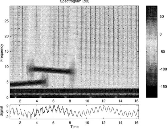
Fig. 2. Spectrogram of the synthetic signal in the noise-free case; frequencies are in h~1

is about 0.23 h~1. Therefore, we clearly see two pure tones, one in the first frequency bin and the second around 2 h~1. The two other important features are two wide peaks of power, the first around 5 h~1 and the second around 9 h~1. These wide peaks cannot be interpreted as pure frequencies in view of the frequency resolution. Fur-ther, without the knowledge of the model, nothing can be inferred concerning these features.

2.1.2 Noisy case

We have added to y(t) a random white Gaussian noise of variance 0.5. The non-stationarity of the signal makes it difficult to give a clear definition of a signal-to-noise ratio. The middle panel of Fig. 1 shows the estimated power spectrum of the noisy y(t) in decibels. The two pure tones are sufficiently powerful to be clearly seen. The two wide peaks are still visible (this is not so clear in the case of the square modulus of the Fourier transform of the data, or periodogram, as seen in the bottom panel of Fig. 1). How-ever, the average induced by Thomson’s method causes a smoothing of these features.

2.2 Non-stationary signal analysis: spectrogram and scalogram

We now turn to time-frequency analysis. Since some of the oscillations seem to vanish after some time, it is useful to analyse EISCAT signals using non-stationary tools. The first we describe is the spectrogram which consists in a time-dependent Fourier analysis; although the spectro-gram is now well known, we think it worthwhile to recall some basics. The second is based on the wavelet transform

and is called the scalogram (Cohen, 1995; Flandrin, 1993; Grossman et al., 1989).

2.2.1 Spectrogram

A natural approach to generalize the spectral analysis of stationary signals to non-stationary signals is to make time dependent the Fourier transform. Hence, the short-time Fourier transform is defined as

Xx(t, l)":h(t!q)x(q)e~2inlqdq, (4)

where h(t) is some window. To obtain an energy inter-pretation, we take the square modulus of the short-time Fourier transform to obtain the spectrogram

SPx(t, l)"D: h(t!q)x(q)e~2inlqdqD2. (5)

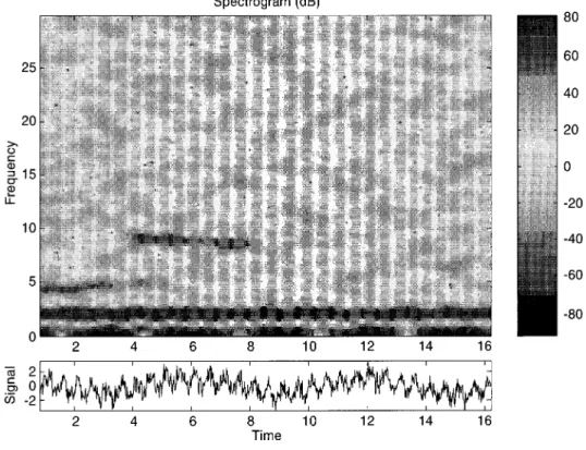
The spectrogram may thus be interpreted as a time-depen-dent spectrum. Its application on the synthetic signal is presented in Fig. 2 for the noise-free case, and in Fig. 3 for the noisy case. These spectrograms have been obtained with a Hamming window of length 100 samples (100 min). Figure 2 clearly depicts the real structure of the syn-thetic signal by showing the two pure frequencies and the two chirps. The time-limited character of the chirps is demonstrated by this analysis, a fact which was neglected by the classical spectral analysis. In the noisy case, things are less evident. The two pure frequencies are clearly visible, but the two chirps are greatly altered by the noise. However, they are still apparent.

The length of window h(t) defines the frequency resolu-tion. The larger the length, the greater the frequency resolution, but the poorer the time localization. It is to be noted that this resolution is constant over all frequencies. For rapid phenomenon, this can be a drawback of the

Fig. 3. Spectrogram of the synthetic signal in the noisy case; frequencies are in h~1

spectrogram, since rapid events will appear ‘‘delocalized’’ in time. A solution to this problem is to use the scalogram. 2.2.2 Scalogram

To overcome the constant resolution of the spectrogram, one wants a tool which gives a good time localization of rapid phenomena and a good frequency resolution for low-frequency events (which are delocalized in time).

The wavelet transform achieves these wishes. For a sig-nal x(t) the wavelet transform reads

¼x(a, b)"_Ja1 : x(t)W*

A

B

In this definition,W is called the wavelet, b is the time-location parameter, a is called the scale and * denotes a complex conjugate;W is typically an oscillating function whose mean is zero.

To obtain an energy representation, we consider the square modulus of ¼x(a,b), which is called the scalogram (Grossman et al., 1989; Flandrin, 1993) and reads

¼x(a, b)"

K

A

B

K

2

. (7)

In this paper, we use the so-called Morlet wavelet which reads

W(t)"ejctMe~t2_@2!J2e~c2_@4e~t2_{N, (8)}

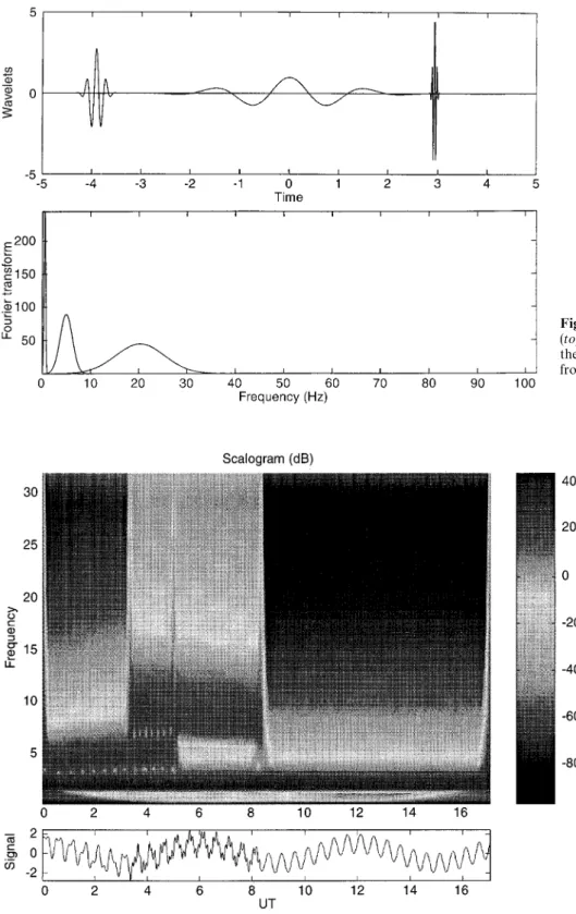
where c is a parameter we will discuss later. We plot at the top of Fig. 4 the waveform ofW (t/a) for some values of the scale: a"1, 1/8 and 1/32, whereas at the bottom appears the modulus of the corresponding Fourier transforms. This figure highlights the behaviour of the wavelet

trans-form: the greater the scale, the greater the frequency res-olution, but the poorer the time localization. Note that large scales correspond to low frequencies, whereas small scales correspond to high frequencies. The behaviour of the Fourier transform of W (t/a) explains why the fre-quency resolution decreases when the scale decreases: the wavelet acts as a filter with a constant surtension factor. Indeed, the wavelet is in general a band pass function whose centre frequency is denoted byl0, see Fig. 4. The scale may be associated to the notion of frequency via

a"l0/l. Hence, it is not universal, since it depends on the

wavelet. All the scalograms are represented here in terms of frequencyl"l0/a.

Parameter c in Eq. 8 is related to the centre frequency l0 of the Fourier transform of the wavelet via l0"c/2n. It therefore defines the band analysis of the scale a"1. Furthermore, c rules the intersection between the band analysis of two different scales: when c is small, about 2, the wavelets at two different scales share a lot of their band (two events which are close in frequency will not be separated). When c is greater, the wavelets at two different scales are more separated in terms of their frequency bands, and therefore two events close in frequency will be more clearly separated. Taking c higher is possible, but Shannon’s Theorem of sampling then forbids the use of very small scales (since the Fourier transform of the dilated wavelet will have its maximum frequency higher than half Shannon frequency). As recommended in Flan-drin (1993), we choose c"5.34, a value which gives a good compromise between the two extreme behaviours explained above.

Finally, parameter a is taken in this paper to be a power of two (octaves). But in order to get a better resolution in scale, we evaluate between two octaves

Fig. 5. Scalogram of the synthetic signal in the noise-free case; frequencies are in h~1

Fig. 4. Some dilated versions of the wavelet (top, from left to right: a"1/4, 1, 1/8) and their Fourier transform in modulus (bottom, from left to right: a"1, 1/4, 1/8)

several ‘‘sub-octaves’’, called tracks. In this paper we evaluate 15 tracks per octave.

The application of the scalogram to the synthetic sig-nals is shown in Figs. 5 and 6 for the noise-free case and the noisy case, respectively.

The features of the synthetic signal clearly appear in the noise-free case. The chirps appear on overlapping inter-vals of scales: this is due to the nature of the wavelet transform as explained in Fig. 4. Moreover, strong

side-effects appear at the edges of the chirp because the wavelet transform has the ability to point discontinuities.

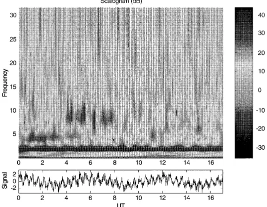
In the noisy case, the overlapping makes the readability of the scalogram poorer than that of the spectrogram. However, comparing the spectrogram and the scalogram allows to confirm the presence of the four features.

The conclusion to this is that several different time-frequency (or scale) analyses should be performed in order to understand the structure of a non-stationary signal.

Fig. 6. Scalogram of the synthetic signal in the noisy case; frequencies are in h~1

The two methods described allow to have two different representations of the same information. Therefore, they allow to confirm or disconfirm some inferences made on the structure of the signal. We now turn to the application of these three analyses on EISCAT signals.

3 Application to EISCAT data

3.1 Detailed analyses of the 24 March 1995 experiment

In order to demonstrate the use of the time-frequency tools of signal processing for EISCAT data, we first select the experiment held on 24 March 1995. It consists in a CP1 experiment that we processed at an integration time of 1 min. The plot of the overall experiment is shown in Fig. 7. It starts at 1300 UT and lasts for about 11 h. The F-region ionosphere starts to become empty at about 1700 UT when the sun sets, until about 1930 UT. Shortly after, soft precipitations occur that last for more than 1 h. They harden around 2030 UT. The effect is clearly seen both on the electron density and temperature. The north-ward electric field exhibits two maxima above 50 mV m~1 at 1940 and 2010 UT while the westward electric field peaks at more than 30 mV m~1 at 2205 UT. Except for these two events, the electric field remains low. The effects of these events are obvious in the ion-temperature plot, with enhancements up to 1600 K at 350 km. In a paper in the same issue (Blelly et al., 1996) some of these events are described in great detail and modelled using a coupled fluid/kinetic transport code.

The ion velocity shows different patterns. From the beginning of the experiment until about 1600 UT, a clear

oscillating pattern occurs from 178 up to 258 km, Fig. 7. This is the pattern we are looking for in order to illustrate the power of time-frequency analysis. From 1730 UT to about 2000 UT, the ion velocity is enhanced at all alti-tudes. Then, no clear structure may be seen from the plots of the ion velocity.

In order to eliminate the noise from our data, we could average the ion velocity at different altitudes. However, the phase of the oscillation moves from one altitude to the other, and the results would not be as explicit. This is why we process the analysis at separate altitudes. The details will be shown at 190.5 km. At this altitude, the time-sequence is shown in Fig. 8.

The first approach is the ‘‘usual’’ one based on the Fourier transform. It has been shown in Sect. 2.1 that such an analysis, based on the assumption of stationarity, is not well suited for sporadic events. This is illustrated in Fig. 9, which represents the periodogram (square modulus of the Fourier transform of the whole data set) in dB. It shows a slight increase at about 1/3 h with an amplitude of about 30 dB. There is no clear other feature. A way to improve this analysis is to filter the signal in order to substract the low-frequency part of the spectrum (typically the 12-h tide). Such a filtering improves the dynamics of the peri-odogram, but does not help in its analysis. Therefore, it is not shown here. Furthermore, this analysis is done with-out any average, and therefore the effect of the noise is strong.

Thomson’s method may be understood as a tricky average of the periodogram. Indeed, the tapering of the data using orthogonal windows greatly reduces the noise. That becomes obvious when one compares the periodo-gram with Fig. 10. The increase at 1/3 h is better extracted,

F ig. 7. Qui ck loo k o f th e sel ect ed expe ri me n t

Fig. 8. Ion velocity (m s~1) at 190.5 km for the 24 March 1995 experiment

Fig. 9. Square modulus of the Fourier transform of the ion velocity; frequencies are in h~1

Fig. 10. Spectrum of the ion velocity; frequencies are in h~1

with probably some additional pattern at 1/4 to 1/5 h. Again, this method, being based on the stationarity as-sumption cannot give further information.

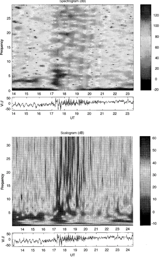
The first time-frequency tool demonstrated here is the spectrogram. We used the same Hamming window of length 60 min. In Fig. 11,we show the spectrogram and the time-series of the ion velocity at the same scale in the bottom panel. This analysis is able to extract different patterns. The first, from the beginning of the experiment to about 1600 UT, is a wave with a period of 18 min (or frequency of 3.3 h~1). Then, from about 1700 UT to about 2000 UT, there is a broadband excitation. The time localization of this pattern is however difficult to deter-mine on this analysis: the length of the analysing window is 60 points, corresponding to 1 h. This means that at both the beginning and the end of each event, there is an uncertainty of half an hour. However, this broadband oscillation occurs before both precipitations and electric-field enhancement. These two perturbations have an effect on the amplitudes of the physical parameters (electron density, temperatures and ion velocity), but do not seem to affect the frequency of the velocity oscillations. Finally, from about 2230 UT to the end of the experiment, a wave at 30 min is excited. This last feature confirms the two stationary analyses, since the spectrum can be roughly seen as a projection of the spectrogram on the frequency axis. The new thing here is that we are now able approxi-mately to locate in time these features.

These observations are confirmed by the scalogram, Fig. 12. The excitation of all frequencies shows up at the same time as on the spectrogram. The low-frequency tides are extracted, and as explained in Sect. 2.2.2, the scalo-gram points on the discontinuities, so that one sees strong side-effects.

Note that on both the spectrogram and the scalogram, the noise induces some quite powerful patterns. A ‘‘thresh-olded’’ image would help to extract the signal patterns from the noise patterns. But we deliberately chose not to present such a thresholded image in order to show the full dynamics.

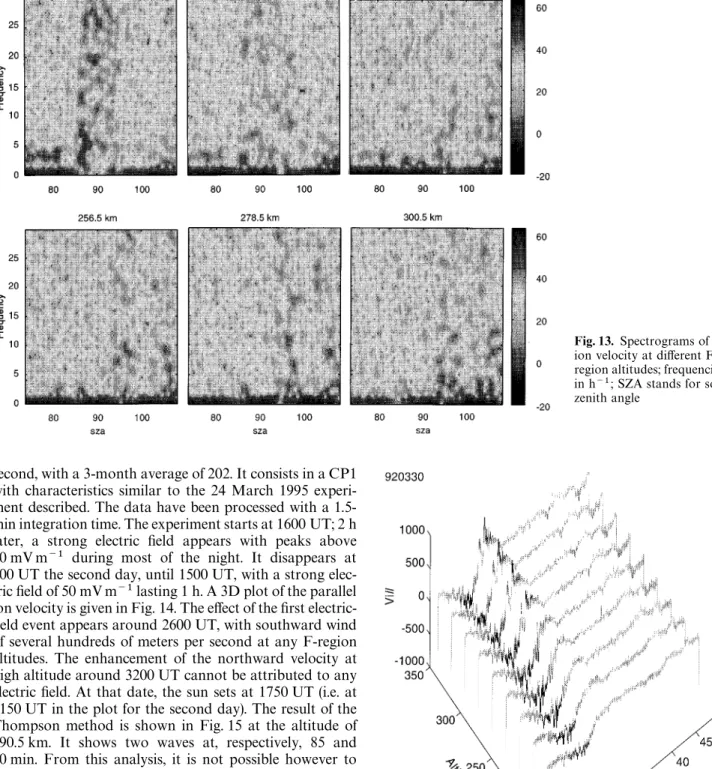
In Fig. 13, we show the spectrograms of the parallel ion velocity at different altitudes in the F region. We plotted the spectrograms in terms of the solar zenith angle instead of UT, to make it easy to locate the different patterns versus sunset. The 18-min oscillation slowly vanishes when one looks at higher altitudes; it is hardly visible at 256.5 km. The same happens to the broad-band pattern: it is centred at 90° of solar zenith angle, i.e. during the sunset. It is of much less amplitude at 212 km and hardly visible above.

3.2 Overview of some other experiments

We performed our analyses for different experiments. Our first choices were two long experiments held in October 1992 and January 1993. The reason for these choices is that these experiments have been compared to different models (Lilensten and Lathuille`re, 1995). However, during these two experiments (respectively, 2 and 5 days), the solar zenith angle hardly reaches 90°, so that it has not

Fig. 11. Spectrogram of the ion velocity; frequencies are in h~1

Fig. 12. Scalogram of the ion velocity; frequencies are in h~1

been possible to observe the sunset broad-band excitation already described. No structured oscillation (faster than 1 h) shows up during these 7 days of experiment. The same observation applies to a summer experiment (5 August 1992), when the sun is always above the horizon: we could not see evidence for a structured fast pattern. These

anal-yses tend to show that the oscillations of the ion velocity (and therefore of the meridional wind) may be compared to geophysical noise.

We now focus on the 36-h experiment held 30—31 March 1992. It is an active experiment, with an Ap index of 12 to 13. The solar index is 192 the first day and 182 the

Fig. 13. Spectrograms of the ion velocity at different F-region altitudes; frequencies are in h~1; SZA stands for solar zenith angle

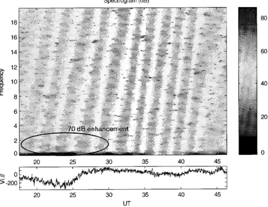
second, with a 3-month average of 202. It consists in a CP1 with characteristics similar to the 24 March 1995 experi-ment described. The data have been processed with a 1.5-min integration time. The experiment starts at 1600 UT; 2 h later, a strong electric field appears with peaks above 50 mV m~1 during most of the night. It disappears at 500 UT the second day, until 1500 UT, with a strong elec-tric field of 50 mV m~1 lasting 1 h. A 3D plot of the parallel ion velocity is given in Fig. 14. The effect of the first electric-field event appears around 2600 UT, with southward wind of several hundreds of meters per second at any F-region altitudes. The enhancement of the northward velocity at high altitude around 3200 UT cannot be attributed to any electric field. At that date, the sun sets at 1750 UT (i.e. at 4150 UT in the plot for the second day). The result of the Thompson method is shown in Fig. 15 at the altitude of 190.5 km. It shows two waves at, respectively, 85 and 50 min. From this analysis, it is not possible however to locate these features in time. Figure 16 shows the spectro-gram of the experiment. The two oscillations occur from the beginning of the experiment to about 2600 UT, with an enhancement at about 2300 UT for the fastest (50 min). This is during the first electric-field event, but there is no clear structured fast oscillation during the second.

4 Discussion and conclusion

In this paper we examined the use of some time-frequency tools for analysing EISCAT data. The spectrogram is easily coded and easily used. However, it requires some experi-ence to choose correctly the length of the analysing window.

Fig. 14. Overview of the 30 March 1992 parallel ion velocity; alti-tudes are in km and the velocity in m s~1

The scalogram has proved to be delicate, but should nevertheless not be forgotten. Its main quality is clearly to extract scale effects in a data set. It is therefore very well suited for fractal behaviour, although that has not been

Fig. 16. Spectrogram of the 30 March 1992 experiment (altitude 190.5 km); frequencies are in h~1

shown here. Its use has proved to be very powerful in other domains of geophysics (see for example Fong Chao and Naito, 1995).

From the few experiments we processed, preliminary conclusions may be drawn: some of the oscillations that seemed to occur at any time when comparing EISCAT meridional winds with interferometer measurements or models could well be coherent and sporadic. In our se-lected data sets, two waves occur during about 2 h in the 1995 experiment, and more than 6 h during the 1992

Fig. 15. Thompson analysis of the 30 March 1992 experiment (alti-tude 190.5 km); frequencies are in h~1

experiment, suggesting that we face ‘‘classical’’ gravity waves, as described in Crowley et al. (1987); these authors compared the morphologies of short-period TIDs for magnetically quiet and active intervals, explaining the differences in terms of perturbed neutral-wind patterns and different wave sources during active times. However, most of the time, the oscillations may be attributed to geophysical noise: we could only extract these few struc-tured oscillations from 15 days of experiments.

It is also interesting to see that all the ion-velocity frequencies seem excited from 1700 to 1930 UT during the 1995 experiment. A stationary analysis only extracts noise, but the spectrogram and scalogram show that this ‘‘noise’’ is a broadband excitation which specifically oc-curs during the sunset.

This study is a first approach, and before useable tools may be given to the EISCAT community, more studies are needed. We also performed our analyses on different para-meters (ion and electron temperatures and electron den-sity). The results are not shown here, since they do not carry any additional information concerning the purpose of this paper, which is to show that the use of non-station-ary tools of signal processing for analysing EISCAT data permits to extract the sporadic behaviour of different patterns in a given data set.

Acknowledgements. EISCAT is an international association

sup-ported by the research councils of Finland (SA), France (CNRS), Germany (MPG), Norway (NAVF), Sweden (NFR) and the United Kingdom (SERC). All the computations presented in this paper were performed at the Centre de Calcul Intensif de l’Observatoire de Grenoble. Nous remercions Wlodek Kofman et Nade`ge Thirion pour d’inte´ressantes discussions concernant ce travail.

Topical Editor D. Alcayde´ thanks St. Buchert and another ref-eree for their help in evaluating this paper.

References

Cohen, L., ¹ime-frequency analysis, Prentice-Hall, Englewood Cliffs, N.J., 1995.

Crowley, G., T. B. Jones, and J.R. Dudeney, Comparison of short-period TID morphologies in Antartica during geomagnetically quiet and active intervals, J. Atmos. ¹err. Phys., 49, 1155—1162, 1987.

Fauliot, V., G. Thuillier, and M. Herse´, Observation of the F-region horizontal and vertical winds in the auroral zone, Ann.

Geophysi-cae, 11, 17—28, 1993.

Flandrin, P., ¹emps-Fre´quence (in French), Hermes, Paris, 1993. Fong Chao B., and I. Naito, Wavelet analysis provides a new tool for

studying Earth’s rotation, Eos, 76, 161—165, 1995.

Forbes, J. M., The lower thermosphere coupling study of the CEDAR and WITS programs, Adv. Space Res., 10(6), 251—259, 1990.

Grossman, A., R. Kronland-Martinet, and J. Morlet, Reading and understanding continuous wavelet transform, in ¼avelets, Eds. J. M. Combes et al., Springer-Verlag, Berlin, Heidelberg, New York, pp 1—18, 1989.

Hedin, A. E., M. A. Biondi, R. G. Burnside, G. Hernandez, R. M. Johnson, T. L. Killeen, C. Mazaudier, J. M. Meriwether, J. E. Salah, R. J. Sica, R. W. Smith, N. W. Spencer, V. B. Wickwar, and T. S. Virdi, Revised global model of thermosphere winds using

satellite and ground-based observations, J. Geophys. Res., 96, 7657—7688, 1991.

Lathuille`re, C., J. Lilensten, W. Gault, and G. Thuillier, The meridi-onal wind in the auroral thermosphere: results from EISCAT and WINDII (submitted to) J. Geophys. Res., 1996.

Lilensten, J., and C. Lathuille`re, The meridional thermospheric neutral wind measured by the EISCAT radar, J. Geomagn.

Geoelectr., 47, 911—920, 1995.

Lilensten, J., G. Thuillier, C. Lathuille`re, W. Kofman, V. Fauliot, and M. Hers, EISCAT-MICADO coordinated measurements of mer-idional wind, Ann. Geophysicae, 10, 603—618, 1992.

Percival, D. B., and A. T. Walden, Spectral analysis for physical

applications: Multitaper and conventional univariate techniques,

Cambridge University Press, Cambridge, 1993.

Thomson, D., Spectrum estimation and harmonic analysis, Proc.

IEEE, 70, 1055—1096, 1982.

Thuillier, G., and M. Herse´, Measurements of wind in the upper atmosphere: first results of the MICADO instrument, in Progress

in Atmospheric Physics, Kluwer Academic Publishers, Dortrecht,

pp 61—73, 1988.

Thuillier, G., and M. Herse´, Thermally stable field compensated Michelson interferometer for measurement of temperature and wind of the planetary atmospheres, Appl. Opt., 30, 1210—1220, 1991.