Statistical atmospheric downscaling for rainfall estimation in Kyushu Island, Japan

HAL Id: hal-00304603

https://hal.archives-ouvertes.fr/hal-00304603

HAL is a multi-disciplinary open access archive for the deposit and dissemination of sci-entific research documents, whether they are pub-lished or not. The documents may come from teaching and research institutions in France or abroad, or from public or private research centers.

L’archive ouverte pluridisciplinaire HAL, est destinée au dépôt et à la diffusion de documents scientifiques de niveau recherche, publiés ou non, émanant des établissements d’enseignement et de recherche français ou étrangers, des laboratoires publics ou privés.

estimation in Kyushu Island, Japan

C. Bertacchi Uvo, J. Olsson, O. Morita, K. Jinno, A. Kawamura, K.

Nishiyama, N. Koreeda, T. Nakashima

To cite this version:

C. Bertacchi Uvo, J. Olsson, O. Morita, K. Jinno, A. Kawamura, et al.. Statistical atmospheric downscaling for rainfall estimation in Kyushu Island, Japan. Hydrology and Earth System Sciences Discussions, European Geosciences Union, 2001, 5 (2), pp.259-271. �hal-00304603�

Statistical atmospheric downscaling for rainfall estimation in

Kyushu Island, Japan

Cintia Bertacchi Uvo

_{, Jonas Olsson}

_{, Osamu Morita}

_{, Kenji Jinno}

_{, Akira Kawamura}

_,

Koji Nishiyama

_{, Nobukazu Koreeda}

_{and Takanobu Nakashima}

2_{Institute of Environmental Systems (SUIKO), Kyushu University, 6-10-1 Hakozaki, Higashi-ku, Fukuoka 812-8581, Japan}

3_{Department of Earth and Planetary Sciences, Faculty of Science, Kyushu University, 6-10-1 Hakozaki, Higashi-ku, Fukuoka 812-8581, Japan} 4_{CTI Engineering Co., Ltd., 2-4-12 Daimyo, Chuo-ku, Fukuoka 810-0041, Japan}

Email:Cintia.Uvo@tvrl.lth.se

Abstract

The present paper develops linear regression models based on singular value decomposition (SVD) with the aim of downscaling atmospheric variables statistically to estimate average rainfall in the Chikugo River Basin, Kyushu Island, southern Japan, on a 12-hour basis. Models were designed to take only significantly correlated areas into account in the downscaling procedure. By using particularly precipitable water in combination with wind speeds at 850 hPa, correlation coefficients between observed and estimated precipitation exceeding 0.8 were reached. The correlations exhibited a seasonal variation with higher values during autumn and winter than during spring and summer. The SVD analysis preceding the model development highlighted three important features of the rainfall regime in southern Japan: (1) the so-called Bai-u front which is responsible for the majority of summer rainfall, (2) the strong circulation pattern associated with autumn rainfall, and (3) the strong influence of orographic lifting creating a pronounced east-west gradient across Kyushu Island. Results confirm the feasibility of establishing meaningful statistical relationships between atmospheric state and basin rainfall even at time scales of less than one day.

Key words: atmospheric downscaling, precipitation, rainfall, singular value decomposition, southern Japan

Introduction

The focus of the present paper is to obtain empirical statistical linkages between smaller-scale (local and regional) hydrometeorology and rainfall in particular, and larger-scale (synoptic and mesoscale) atmospheric circulation. Generally, the strength of such linkages expresses the relative importance of synoptic circulation and local modification, respectively, in determining the smaller-scale hydrometeorological process. If sufficiently strong, the linkages may perform what has been termed (atmospheric) downscaling, i.e. to estimate a point- or spatially-averaged value of some hydrometeorological variable within a specified time interval, on the basis of large-scale features of the surrounding atmospheric circulation. In recent years, the interest in atmospheric downscaling to transport the output of general circulation models (GCMs) to hydrologically relevant (catchment or sub-catchment) scales (e.g. Wilby and Wigley, 1997) has

increased considerably. Statistical downscaling of GCM outputs has been advocated as a less computer-intensive and less time-consuming alternative to the development and application of regional models, nested in the GCM (e.g. Hewitson and Crane, 1996). However, a further alternative is to combine regional modelling with statistical downscaling. Even if the regional model may increase the spatial resolution to as high as 0.05°×0.05°, (1) the distance between a catchment and nearest grid node may still be large, and (2) specific geographical and topographical catchment characteristics that influence the rainfall process strongly are still highly smoothed in regional models. Moreover, as for atmospheric models in general, the output accuracy is substantially higher for free atmosphere variables than for rainfall (e.g. Giorgi and Mearns, 1991). The integrated effect is that estimating catchment rainfall on the basis of model rainfall output is associated with high uncertainties. It is hypothesised that catchment rainfall estimation can be improved by statistical downscaling.

Within the statistical atmospheric downscaling approaches made to date, two principally different groups may be distinguished (e.g. Conway and Jones, 1998). In one of these, the atmospheric circulation pattern is classified as belonging to a certain ‘weather type’, and the observed statistics of each weather type forms the basis from which stochastic downscaling of future circulation patterns is performed (e.g. Hay et al., 1991; Bardossy and Plate, 1992; Wilby, 1994). This approach has been advocated due to its physical transparency (e.g. Conway and Jones, 1998) but suffers from limitations such as the subjectivity inherent in the classification procedure and the inevitable loss of information when generalizing the continuously changing atmosphere into a finite set of classes (e.g. Wilby, 1994; Hewitson and Crane, 1996). The second group of approaches comprises attempts to establish direct statistical relationships between (continuous) variables representing the large-scale state of the atmosphere and the local and regional hydrometeorology (normally temperature and/or rainfall). Numerous statistical techniques have been employed in the identification of optimal relationships, including single and multiple regression, canonical correlation analysis, and artificial neural networks (e.g. Karl

et al., 1990; von Storch et al., 1993; Wilby et al., 1998b).

The strength of statistical relationships linking atmospheric circulation to local and regional rainfall amounts are likely to depend on the time scale involved. Much work has concerned a monthly time scale. Very generally, values of explained variance reaching 0.75 have been found, with a clear dependence on geographical location, time of the year, and the variable used to represent the atmospheric circulation (e.g. Weare and Hoeschele, 1983; Cayan and Roads, 1984; Wigley et al., 1990). These results confirm the feasibility of the approach but a monthly time scale is relevant in a climatological rather than hydrological context. Recently, investigations focusing on a daily time scale have been carried out. As expected, the explained variance has been substantially lower in these studies, with values up to 0.45 (e.g. Kidson and Thompson, 1998; Wilby et al., 1998a). Also, the spatial extension, location, and resolution of the grid points used to define the state of the atmosphere are likely to influence the relationships but this issue appears to have been addressed in only a few investigations (e.g. Weare and Hoeschele, 1983).

To date, virtually all investigations of statistical downscaling have been undertaken in regions in either North America or Europe and there is an urgent need to test the approach in other climate regions. The present investigation concerns northeast Asia, southern Japan in particular. For this region, only a handful of related papers appears to have

been published. One example is Wilby et al. (1998a), who used airflow indices (vorticity, flow strength and direction) to downscale a range of hydrometeorological variables on a daily basis in central Japan using both observed and GCM generated sea-level pressures. Rainfall amounts and sequential characteristics were shown to depend on the vorticity index and, based on these results, a statistical model was developed which, depending on the season, explained ~20-45% of the variance (Wilby et al., 1998a). Hirakuchi and Giorgi (1995) used a nested regional model to downscale daily GCM output in eastern Asia, with emphasis on the Japanese Islands. Although the representation of some space-time features of the regional rainfall was improved by the regional model, the estimation accuracy of rainfall amounts was comparable to simple interpolation of the GCM output (Hirakuchi and Giorgi, 1995). The fairly limited success of these approaches emphasizes the region’s complex atmospheric dynamics and the necessity for further investigations.

Experimental setup

STUDY REGION

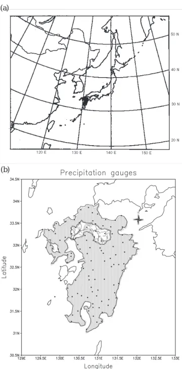
Kyushu Island, the southernmost of the four main Japanese islands, has been used as the study region in the present experiments (Fig. 1). The most important topographic feature of Kyushu Island is the Kyushu mountains aligned in a north-south direction at the centre of the island. The spatial distribution of precipitation depends largely on the direction of prevailing winds relative to the orientation of this mountain range. The annual precipitation and its seasonal distribution at four meteorological stations are shown in Table 1. The stations are Fukuoka, Kumamoto, Miyazaki and Kagoshima, which represent the northern, western, eastern and southern parts of the island, respectively.

In spring, the most important meteorological phenomena affecting Kyushu are transient mid-latitude synoptic cyclones that develop along polar fronts. Japan is located eastward from the Eurasian continent and a semi-permanent upper trough lies over the Japanese Islands. This upper trough increases the cyclones’ activity as they progress along a well-defined storm track over the East China and Japan seas. Synoptic cyclones bring much precipitation (20~30% of the annual total) which is distributed almost uniformly all over Kyushu Island, except that the amount of rainfall is slightly larger over southern than northern Kyushu.

In early summer, polar fronts become active south of Kyushu. These are called Bai-u fronts in Japan and Mei-yu fronts in China. Southwesterly winds caused by the Pacific High convey warm and moist tropical air to the fronts. In

this situation, mesoscale rainbands are formed over the Bai-u fronts and large amounts of rain falls over Kyushu. Due to the preferential wind direction, the amount of rainfall is larger at the western slope of the Kyushu mountains than at the eastern slope. In addition to the rainbands, mesoscale cyclones originating from subtropical depressions migrate eastward along the Bai-u front. The front gradually displaces northward and the Bai-u season comes to an end over northern Kyushu in mid-July. Much rain (25~30% of the annual total) falls in this season. Later in the summer, the summer monsoon influences Kyushu Island. Precipitation is brought about by the prevailing warm and moist southwesterly winds alternating with periods of clear sky caused by the westward expansion of the Pacific High, the Ogasawara High. This period is drier than the early summer and precipitation is basically of a convective and localised nature.

During autumn, the meteorological situation resembles that of spring except for the passage of typhoons. Typhoons bring much precipitation to southern and particularly eastern Kyushu. As the rainbands accompanying typhoons are located at the eastern side of the typhoon centre, typhoons which cross the west of Kyushu Island bring heavy rainfall to the east side of Kyushu mountains. Typhoons crossing the east of Kyushu Island do not cause heavy precipitation and, consequently, eastern Kyushu is affected more by typhoons than other parts of the island.

In winter, the climate is dominated by the winter monsoon. The northwesterlies bring heavy snowfall to the Japanese Islands, especially in the northern part of Honshu Island. The cold and dry northwesterlies become moist while passing over the Japan Sea which is relatively warm owing to a branch of Kuro-shio, a warm tropical ocean current. The situation is somewhat different in Kyushu since the Korea and Tsushima Straits are so narrow that cold and dry northwesterlies cannot obtain much moisture while in transit. In consequence, only a little snowfall is observed in northern Kyushu. On the other hand, northwesterlies blow over the East China Sea and bring heavier precipitation to the southern part of Kyushu. In late winter, cyclones (called

Table 1. Climatological (1961 – 1990) annual precipitation totals and the percentage of precipitation during

each season for four stations on Kyushu Island.

Name Location Annual Prec. Spring Summer Autumn Winter

Fukuoka 33.6N 130.2E 1604.3 mm 23.0% 42.4% 21.9% 12.7%

Kumamoto 32.8N 140.3E 1967.7 mm 24.6% 50.0% 16.3% 9.5%

Miyazaki 31.9N 131.4E 2434.6 mm 26.9% 39.4% 25.6% 8.0%

Kagoshima 31.6N 130.6E 2236.8 mm 29.0% 41.0% 18.3% 11.7%

Fig. 1. Area covered by GPV meteorological data with Kyushu

Island marked in black (a), and distribution of AMeDAS precipi-tation sprecipi-tations in Kyushu Island and the Chikugo River Basin (b).

(a)

south coastal cyclones or Taiwan depressions) develop very rapidly bringing heavy snowfall to southern Kyushu.

In the present study, rainfall forecasting for the Chikugo River Basin is taken as a case study. The Chikugo River originates from the outer rim of Mt. Aso caldera in the central part of the island (Fig. 1b). The range in altitude within the basin is from 0 to 1791 m.a.s.l. (Mt. Kuju), large considering the 143 km length of the main stream. In addition, 70% of the basin comprises mountain ranges of different altitudes while the remaining 30% consists of plains.

Besides being a main city water resource, the discharge of the Chikugo River plays an important role in agriculture, fishery and industry. However, devastating floods and debris flow occur often after heavy rains during the rainy and typhoon seasons from June until October. The annual ratio of maximum to minimum discharge at the Senoshita gauging station ranged from 47.2 to 283.5 for the period 1975 to 1994, but historical records indicate ratios as high as 3750. This fact stems from the steep mountain slopes and the steep river bed gradient, which cause quick arrival and high peak discharge after heavy rainfall. On the other hand, prolonged periods with only small rainfall amount lead to very low flow levels. The average discharge at the Senoshita station, with a catchment area of 2315 km2_{, is 114.7 m}3_s-1 _{and may}

drop to levels as low as 10 m3_s-1_{, as was the case in 1978,}

causing a devastating lack of water in surrounding cities. Hence, a detailed understanding of both flood and drought characteristics of the Chikugo River Basin is important. For this purpose, advanced hydrological modelling of drought risks and countermeasures is presently being carried out (e.g. Merabtene et al., 1998). Further, effective flood monitoring systems integrating radar and rain-gauge observations, river water levels and large-scale meteorological information are under development to establish more robust flood warning. The present study constitutes the first part of a series of experiments assessing the role of atmospheric downscaling in this system development.

DATA BASES

The atmospheric data used in these experiments consisted of the grid point meteorological data (GPV) used as input to the Japan Meteorological Agency’s regional weather forecasting model. The area covered includes Japan and surrounding seas, South and North Korea, eastern China, eastern Mongolia and the southern parts of easternmost Russia (Fig. 1a). The data consist of sounding measurements at 00Z and 12Z, which were interpolated into a 217×257 point grid of 20×20 km resolution grid by optimum interpolation (e.g. Daley, 1991). The GPV meteorological variables include sea level pressure, geopotential height,

zonal and meridional wind speeds, temperature and dew point depression, available at surface and 20 vertical levels up to 10 hPa (11 vertical levels up to 300 hPa for dew point depression). In the present analysis, values at surface, 850 hPa, 500 hPa and 250 hPa were used. At these levels, vorticity was derived directly from the wind field. Additional derived variables were calculated such as precipitable water, obtained by vertical integration of humidity, and total-totals index, a vertical stability index defined by:

where t_d denotes dew point temperature, t temperature (both in degrees Celsius), and the numbers in brackets denote level (in hPa). These variables are closely related to the origin of precipitation and thus our interest in examining their performance as predictors in a statistical model.

For the present study, data observed during 21 months extending from April 1996 to December 1997 were available. The total number of time instants (12-hour periods) was 1265. In the present analysis, the grid points were averaged 5×5 (resolution: 100×100 km) into a 43×51 grid point network and 25×25 (500×500 km) into an 8×10 network. The averaged grid point values were obtained as the arithmetic mean of the original grid point values contained in the averaging area.

The rainfall data employed were collected by the Japanese national meteorological network (AMeDAS). In this network of 1313 stations covering all of Japan, rainfall is measured hourly. The total number of AMeDAS stations on Kyushu and surrounding islands exceeds 150 but, in the present study, data from some stations were disregarded either because the time series contained extended periods with missing data or if two stations were very closely located and thus likely to contain essentially the same signal (in this case the station with the more complete data was used). After this screening, 103 stations remained. Figure 1b shows the distribution of the stations over Kyushu Island. For the period April 1996 to December 1997 missing values from these stations amounted to 3%. This percentage is considerably lower than the limit of 10% suggested by Lau and Sheu (1988) as the amount that would compromise the results of a statistical analysis. These missing values were replaced by the values from the nearest functioning station when an objective comparison between the two series showed that this replacement could be made safely.

To obtain spatial rainfall representative of the Chikugo River Basin, hourly arithmetic averages from the 11 stations located within and in the immediate vicinity of the basin were calculated. The location of Chikugo River Basin and the distribution of these stations can be seen on Fig. 1b. While fairly evenly distributed spatially, the precipitation

[ ] [ ]

(

)

(

)

stations available are not evenly distributed in terms of altitude. Only one of the 11 stations is located above 1000 m.a.s.l, two are located between 300 and 500 m, and the remaining eight are below 150 m.

To agree with the temporal resolution of the GPV data, the hourly rainfall data were accumulated into 12-hour values. Two strategies were tested:

l starting the accumulations at the GPV observation times (00Z and 12Z), assuming a relationship between the state of the atmosphere and rainfall during the following 12-hour period;

l starting the accumulations six hours before the GPV observations (06Z and 18Z), assuming a relationship between the state of the atmosphere and rainfall during the surrounding 12-hour period.

To investigate seasonal differences, the data were split into seasons: winter (Dec-Feb), spring (Mar-May), summer (Jun-Aug), and autumn (Sep-Nov). The number of time instants for each season was 241, 292, 368 and 364, respectively.

Methodology

Singular Value Decomposition (SVD), used for the analyses and downscaling model development in this work, is a multivariate technique that isolates linear combinations of variables within two fields that tend to be linearly related to each other. As a result, SVD provides spatial patterns from the two fields that explain most of the covariance between them. SVD was chosen for this study both for being simple and straight forward to apply and for its documented applicability to co-varying hydro-meteorological fields. It requires low computational performance and can be run easily on micro computers. Using a statistical model applied to circulation and moisture fields generated by a regional physical model avoids the use of parameterisations that are, in general, a weakness of physically-based models.

The first use of SVD for identifying the relationship between two meteorological fields was made by Prohaska (1976). Thereafter, not many studies using SVD to relate geophysical fields were published until Bretherton et al. (1992) and its companion paper, Wallace et al. (1992). Then the use of SVD for geophysical purposes increased considerably (e.g. Wallace et al., 1993; Uvo and Berndtsson, 1996 and Uvo et al., 1998). Jackson (1991) and Preisendorfer (1988) present a thorough description of SVD theory and Newman and Sardeshmukh (1995) outline some of the problems to be considered when using SVD to recover the relationship between two fields.

THE METHOD

SVD is applied to two data sets Y_t,y and Z_t,z where time t has nt time steps, necessarily the same for Y and Z. The spatial dimensions y and z have ny and nz points in space, respectively, that do not need to be the same.

The aim of SVD is to find spatial patterns G and H that are linear combinations of Y and Z, respectively and explains most of the total covariance between U and V, i.e.:

U=YG (1)

V=ZH (2)

The cross-covariance matrix of Y and Z is defined as C

nt Y Z

YZ = ₋

1

1 '

, where Y’ is Y transpose, which means that: cov( , ) ' ' max , U V U V nt _{t nt}U Vt t =< >= − ₌

∑

Applying (1) and (2) in (3) gives:

max ' ' ' 1 1 ' = = − >= < GY ZH GC H nt V U YZ (4)

The equation system formed by (1), (3) and (4) is the basis for the SVD calculation and must be solved for G and H. The solution for this system is given by:

(C_YZC_ZY-s2_I)G=0

where σ2 _{are the eigenvalues of C}

YZCZY and G the

eigenvectors (details of this development can be found in Uvo and Graham, 1998).

When SVD is applied to the C_YZ cross-covariance matrix between two fields — in the present case, GPV variables and precipitation — it identifies the pairs of spatial patterns which explain most of the temporal covariance between the two fields.

The results from the SVD are in the form of homogeneous and heterogeneous correlation maps. The kth _homogeneous

map is defined as the vector of correlations between the grid values of one field and the kth _{mode of the singular}

vector (eigenvector) of the same field. Similarly, the kth

heterogeneous correlation map is the vector of correlations between the grid values of one field and the kth _{mode of the}

singular vector of the other field. The homogeneous correlation map is an indicator of the geographic localisation of covarying parts of the field while the heterogeneous correlation map indicates how well the grid points of one field relate to the kth _{expansion coefficient of the other. To}

determine if the correlation coefficients from the homogeneous or heterogeneous correlation maps differ

significantly from what may be expected due to chance, a test of the null hypothesis based on Student’s t distribution can be performed (Bendat and Piersol, 1986).

To compare the strength of the relationship between the GPV and precipitation fields in modes obtained from different SVD expansions within the same season, the normalised squared covariance was used, defined as:

2 / 1 2 var var _         =

∑∑

where var_i and var_j are the variances at the ith _{grid point in}

the GPV field and the jth _{grid point in the precipitation field,}

respectively, and σk2 is the total squared covariance

explained by a single pair of patterns (G_k,H_k). The NSC ranges from 0, when the two fields are unrelated, to 1, when the variations at each grid point in the GPV field are perfectly correlated with the variations at all grid points in the precipitation field.

MODEL DEVELOPMENT

SVD can be used to develop specific prediction or specification models for a particular point in one field (precipitation, in the present case) based on the spatial pattern or on the evolution patterns of the anomalous values in the other field (GPV).

The model was generated by first calculating a matrix of regression coefficients (S) which relates the canonical mode temporal amplitudes of the GPV field (U) to the individual points in the precipitation field (Z). Due to the orthogonality and unit variance of U, these coefficients are given by S_m,z = <U_mZ_z> where m denotes the canonical mode index and z the spatial index of the elements of Z. That is, S_m,z links the GPV side of the canonical mode m to point z in the precipitation field. Thus, denoting the estimates of Z as Zˆ

in matrix form the regression equation becomes Zˆ=U’S. This will be referred to as the SVD downscaling model.

To assure that only the main features of the temporal and spatial variations of the fields will drive the model, two main restrictions were included. First, not all modes of U were used in the model development. Keeping only those modes that are statistically or physically significant (four modes in the present case) avoided the model calibration being influenced excessively by noise. Moreover, as the time step used in the downscaling experiments is 12 hours, a second restriction related to the space was made. To avoid the influence of irrelevant synoptic structures on the downscaling, not all grid points of the GPV space were used in the model. Only the GPV grid points that were statistically

significant at 95% or more on the first mode of the GPV heterogeneous correlation maps were employed in the construction of the model.

Some further adjustment was also required. As the downscaled variable is precipitation, negative values generated by the model were considered as zero. After this adjustment, the model showed a very good performance in determining the timing of the precipitation; however, there remained a tendency to underestimate peaks of precipitation. It is hypothesised that this may be due to the strongly non-linear character of extreme precipitation occurrences. As SVD is a linear method, it is unable to reproduce the non-linear response to changes in the atmospheric forcing associated with extreme events. To compensate for this limitation of SVD, a multiplicative correction factor was applied to the model output to represent the intensity of heavy precipitation better. For this factor, the value 1.2 gave the best general performance over all seasons.

The application of SVD requires (1) normalised data and (2) the summation of the values in each column of the data matrix to be zero. To fulfill these two conditions, the GPV time series at each grid point was normalised by subtracting the average and dividing by the standard deviation. For the precipitation data, however, a more elaborate normalisation was required as the small time step implies numerous observations with zero precipitation. In this case, four steps were followed:

l 0.1 was added to each precipitation value,

l the base-10 logarithms was applied to the values,

l 1 was added to the result of the logarithms with the only purpose of having a minimum value of 0 for the normalised precipitation, and

l the resulting time series were standardised by extracting the average and dividing by the standard deviation. This pre-treatment of data ensured that the precipitation data also fulfilled the requirement for the application of the SVD.

Each season was analysed separately because of the different meteorological mechanisms that influence the area studied. This seasonal splitting improved the results of the downscaling significantly. The seasonal time series were further divided into one calibration and one validation part, with about 80% of the total series in the former.

Results and discussion

SVD models were applied to estimate average precipitation in the Chikugo River Basin by downscaling from atmospheric variables using a 12-hour time step. The data

used for the development of the models were seasonal meteorological fields pre-processed as described earlier. Two spatial resolutions of the GVP data were used: 100×100 km and 500×500 km. These two resolutions were chosen to assess the effect of resolution degradation on the downscaling capacity of the model. Concerning the accumulation strategy, results for accumulations only at 00 and 12Z, i.e. the GPV observation times, are presented as they proved superior and, furthermore, are of most interest in actual model application.

For all seasons, models were generated using all available GPV variables at selected altitudes. In general, best results were achieved at 850 hPa and at 250 hPa, except for temperature for which surface level data brought more significant results.

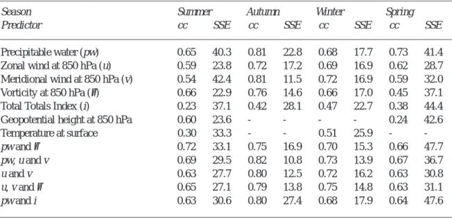
Table 2 presents the correlation coefficients between observed and estimated normalised precipitation and the sum of the squared error (SSE) during the validation periods for the best performing models.

Figure 2a–d shows chosen plots of observed and estimated normalised average precipitation for Chikugo River Basin for summer, autumn, winter and spring, respectively.

Table 2. Correlation coefficient (cc) and sum of squared error (SSE) between the estimated and observed

normalised precipitation during the validation period for different models and seasons (dash indicates that no significant correlations were found on the first mode of the GPV heterogeneous correlation map).

Season Summer Autumn Winter Spring

Predictor cc SSE cc SSE cc SSE cc SSE

Precipitable water (pw) 0.65 40.3 0.81 22.8 0.68 17.7 0.73 41.4

Zonal wind at 850 hPa (u) 0.59 23.8 0.72 17.2 0.69 16.9 0.62 28.7

Meridional wind at 850 hPa (v) 0.54 42.4 0.81 11.5 0.72 16.9 0.59 32.0

Vorticity at 850 hPa (ζ) 0.66 22.9 0.76 14.6 0.66 17.0 0.45 37.1

Total Totals Index (i) 0.23 37.1 0.42 28.1 0.47 22.7 0.38 44.4

Geopotential height at 850 hPa 0.60 23.6 - - - - 0.24 42.6

Temperature at surface 0.30 33.3 - - 0.51 25.9 - -pw and ζ 0.72 33.1 0.75 16.9 0.70 15.3 0.66 47.7 pw, u and v 0.69 29.5 0.82 10.8 0.73 13.9 0.67 36.7 u and v 0.63 27.7 0.80 12.5 0.72 16.2 0.63 30.8 u, v and ζ 0.65 27.1 0.79 13.8 0.75 14.8 0.63 31.1 pw and i 0.63 30.6 0.80 27.4 0.68 17.9 0.64 47.6

Fig. 2. Observed (solid line) and model generated (dashed line)

normalised average precipitation in the Chikugo River Basin during the validation period for: summer (a), autumn (b), winter (c) and spring (d). Model generators for (a) to (c) were zonal and

meridional winds at 850 hPa, and precipitable water. For (d), model generator was only precipitable water. The number on the top left is the correlation coefficient between the two series, and the one on the

MODEL RESULTS

Results showed that the SVD technique was efficient in downscaling precipitation from GPV data specified at a 100×100 km resolution. The accuracy, however, depended on the meteorological variable employed. In general, for all four seasons, vorticity (ζ) and zonal (u) and meridional (v) winds at 850 hPa and precipitable water (pw) produced the best results. Fields such as sea level pressure, geopotential height, temperatures and total-totals index proved very inefficient as precipitation estimators for the region studied at this short time scale. Future references to u, v and ζ are at 850 hPa, unless otherwise stated.

For summer, the best correlation coefficients (cc) between observed and estimated series resulted from using pw and ζ (0.79, 99% statistically significant), and using pw, u and v (0.69, 99% statistically significant) (see Table 2 and Fig. 2a). Although results from the model driven by ζ together with pw resulted in a higher correlation, the timing of the precipitation events as well as the intervening dry periods were represented better when u and v substituted ζ in the model generation. This is also evident from the decrease in SSE (Table 2).

The best performing downscaling experiments were achieved during the autumn. Also, for this season, u and v in combination with pw proved to be the most efficient model generator. Models driven by v and pw alone were very effective in determining the timing of precipitation events (cc = 0.81 – Table 2). However, the model driven by pw only was unable to estimate the intensity of the precipitation, and the SSE of its validation (22.8) is approximately twice as large as the one for v (11.5). When using u and v and pw to drive the model, cc for the validation period increases to 0.82 and the SSE decreases to 10.8 (Fig. 2b). The model represents the timing of precipitation occurrence very well but shows a slight tendency to underestimate the amount.

During winter, the best estimators were pw, and u, v and

ζ. When a model is generated by each of these parameters separately, the resulting cc for the validation period ranges from 0.66 to 0.71 with SSE of about 17.0 (Table 2). However, results improve when the parameters are combined. Using pw and ζ to drive the model, cc for the validation period reaches 0.70 with a SSE of 15.3. Substituting ζ by u and v, cc increases to 0.73 and SSE decreases to 13.9 (Fig. 2c). Results from the model driven by temperature at either surface or 850 hPa during winter were very poor. The cc was 0.51 and SSE 25.9 for the surface case and 0.02 and 30.3 for 850 hPa, respectively. The winter monsoon is less efficient in causing precipitation over southern Japan during winter, but synoptic disturbances have

more influence on precipitation during this season. Best results in spring were reached by the model driven only by pw. In this case, cc for the validation was 0.73 and SSE 41.4. These numbers indicate that the model catches the timing of the precipitation but the amount of precipitation is not equally well represented (Fig. 2d).

In a subsequent test, all the model generations described were repeated using the GPV data for a 500×500 km resolution. As expected, the correlations between observed and estimated normalised precipitation decreased substantially as compared with a 100×100 km resolution. For summer, using pw, u and v to generate the model, cc for the validation period decreased from 0.69 (for 100×100 km GPV) to 0.46 and the SSE increased from 29.5 to 46.4. For the autumn case, using a model driven by pw, u and v, cc decreased to 0.57 and SSE increased to 18.6. In winter, using the same three atmospheric parameters as for the 100×100 km resolution, cc decreased to 0.63 and SSE increased to 22.8. For spring, using only pw to drive the model, the correlation decreased from 0.73 to 0.46 and the SSE from 41.4 to 37.4. The SSE decreased in this case because, estimated by the model, the precipitation was smaller for the whole validation period. This makes periods without precipitation better represented, but the amount of precipitation during events was very poorly estimated (not shown).

Finally, a test was made driving the model with the whole data series, i.e. without seasonal splitting. This model is still able to downscale precipitation with high accuracy during summer and autumn, whereas downscaling for winter and spring is very poor. This is related to the intensity of the signal caught by the SVD analysis. When the whole series is used, the first four modes of the SVD capture the predominant signals related to the summer and autumn seasons, but not the weaker signals of the winter and spring. This result justifies the division into seasons when downscaling precipitation in the Chikugo River Basin.

ANALYSIS OF MODEL RESULTS

Relationships between the various GPV fields and the Kyushu Island precipitation field were analysed by SVD for each season separately and for the whole period. By these analyses, it was possible to assess the influence of the governing physical processes on the downscaling process and understand better the intra-annual variation in downscaling model performance. As in the model development, when analysing the whole lumped period, the strong characteristics of summer and autumn dominate the correlation maps entirely, and not even in lower modes do winter or spring features show up. However, for seasonal

detectable.

SUMMER

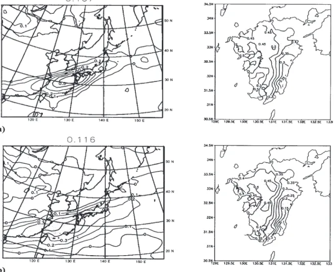
Precipitation over Kyushu Island during summer time is caused mainly by the presence of the Bai–u front. The SVD analysis for the summer season captured this feature very effectively. It appears clearly in the first mode of the GPV heterogeneous correlation maps between pw and Kyushu precipitation (Fig. 3a left) and between u and precipitation (Fig. 3b left) as an area of positive correlations elongated in an east-west direction. An elongated core of significant correlations reaching 0.5 in the pw map and 0.4 in the u map, located in and just southeast of Kyushu Island, can be seen on the GPV correlation maps (Fig. 3a and b left). This feature is positively correlated to precipitation in all parts of Kyushu (Fig. 3a and b right).

The east-west correlation gradient over Kyushu on the

precipitation heterogeneous correlation map (Fig. 3a and b right) is interesting. The highest correlations are observed at the western side of the island reaching values up to 0.5, and in the southwestern tip, where the annual total precipitation is above 2000 mm with 30% of it occurring during this season (Table 1). Lower values are observed in the eastern part of the island. This gradient expresses the difference in precipitation between each side of the main mountain chain extending in a north-south direction in the central part of Kyushu. As the predominant winds during summer are from the southwest, the eastern part of the island is leeward and thus receives less precipitation. The gradient was a constant feature in all the summer precipitation heterogeneous correlation maps analysed.

AUTUMN

Fig. 3. Heterogeneous correlation maps between precipitation over Kyushu Island, and precipitable water (a) and zonal winds at 850 hPa (b)

for summer. Maps to the left are related to GPV fields, and maps to the right to precipitation fields. Shaded areas indicate correlation significance equal to or higher than 95%. Positive correlations are represented by continuous lines and negative by dashed lines. The number

Fig. 4. Heterogeneous correlation maps between precipitation over Kyushu Island, and precipitable water (a), zonal winds at 850 hPa (b), and

The heterogeneous correlation maps for this season show a very strong correlation between meridional winds and Kyushu precipitation (Fig. 4c). This represents the influence of synoptic disturbances from the south, following the storm track over the Japan Sea, bringing precipitation over the whole of Kyushu Island (Fig. 4c right).

Another important characteristic may be observed from the zonal winds/precipitation correlation maps (Fig. 4b). The east-west correlation gradient present on the precipitation map (Fig. 4b right) with higher values to the east shows the difference in precipitation between each side of the mountain chain caused by the passage of typhoons. The zonal wind correlation map associated with this precipitation map is, however, difficult to relate to typhoon activity, mainly due to the discrepancy between the typical size of a typhoon and the spatial extension and resolution of the GPV field used in the present study.

A further main characteristic may be seen from the pw correlation map which shows a core of correlations up to 0.5, in and surrounding the island, positively correlated to the precipitation in all parts of Kyushu Island (Fig. 4a).

WINTER

The main characteristic of the winter season in Japan is the presence of the winter monsoon that comes from the north and brings cold air and precipitation, mainly to the northern part of the country, at the beginning of the season. For Kyushu, however, precipitation during the winter season is brought by synoptic disturbances coming from the southwest, from the so-called Taiwan low.

The zonal and meridional wind fields for winter are somewhat similar to those for autumn but show a lower activity of synoptic disturbances. This agrees with what is observed climatologically. Analyses for winter showed that the heterogeneous correlation maps of pw, u and v explained most of the covariance (NSCs of 0.157, 0.122 and 0.163, respectively, not shown). The three fields are related to precipitation mainly in the central part of the island where correlations in the precipitation heterogeneous map reach values as high as 0.55 around the Mt. Aso region.

The pw correlation map shows that the precipitable water over and around the island is an important factor influencing precipitation. Correlations up to 0.6 on the pw correlation map are positively correlated to precipitation in Kyushu. The precipitation correlation map shows correlations up to 0.55 in the central and southern part of the island. Also the southerly winds over Kyushu were correlated positively with the precipitation. The zonal wind correlation map indicates that the easterly winds in a region northeast of Taiwan are positively correlated to the precipitation in the whole of Kyushu, with higher correlations occurring in the central

part of the island.

SPRING

During spring, the highest NSCs were obtained for v, u and

pw (0.164, 0.153 and 0.144, respectively). These results

express the influence of synoptic disturbances on the precipitation during the season. The precipitation correlation maps (not shown) show that precipitation is spread all over Kyushu during this season, with higher correlations in the higher-altitude parts of the island. This characteristic is also clearly present in the ζ correlation map (not shown).

During this season, as in winter, precipitation over Kyushu is positively correlated with pw and northward winds in and around the island, and zonal winds northeast of Taiwan. In spring, however, precipitation is negatively correlated to zonal winds over the Pacific, east of Kyushu. Contrary to the situation in autumn and winter, the zonal wind map indicates a convergence region near Kyushu Island.

Summary and conclusions

Linear regression models based on singular value decomposition, SVD, were developed for downscaling atmospheric variables statistically to estimate average rainfall in the Chikugo River Basin, Kyushu Island, southern Japan, on a 12-hour basis. The atmospheric data, obtained from sounding measurements, were interpolated in a 100×100 km grid point network covering north-east Asia. In the downscaling procedure, the models were designed to take into account only significantly correlated areas between atmospheric and precipitation fields identified by the SVD. By using as predictors precipitable water in combination with wind speeds at 850 hPa, correlation coefficients between observed and estimated precipitation values exceeding 0.8 were reached.

The capability of the models in forecasting precipitation (represented by the correlation coefficient between observed and estimated values) exhibited a seasonal variation. Better results were observed in autumn and winter than during spring and summer. Using a 500×500 km resolution grid as input showed tendencies similar to the results from a 100×100 km resolution, but correlations between observed and estimated precipitation dropped by ~0.2.

The SVD analysis preceding the model development highlighted important features of the rainfall regime in southern Japan. In particular, (1) the so-called Bai-u front which is responsible for the majority of summer rainfall, (2) the strong circulation pattern associated with autumn rainfall and (3) the strong influence of orographic lifting creating a pronounced east-west gradient across Kyushu Island.

Results confirm the feasibility of establishing meaningful statistical relationships between atmospheric state and basin rainfall even at time scales of less than one day. This, however, requires meteorological grid point value (GPV) data at a resolution of 100×100 km or higher for the area studied.

Concerning weather forecasting, the use of statistical downscaling from free-atmosphere variables is an interesting alternative to the conventional parameterisations of rainfall, considering the present phase of development of parameterisation schemes. Comparative studies between physically and statistically downscaled rainfall from identical atmospheric GPV input, are currently being carried out for the present region. Preliminary results indicate a similar but slightly higher accuracy for the downscaled rainfall, and these results will be reported elsewhere.

Comparing results obtained from downscaling from resolutions of 100×100 km and 500×500 km, respectively, it seems doubtful whether downscaling from 500×500 km grid can be of practical use at such short time scales, at least in this region. However, by nesting a regional model in the GCM, the spatial resolution of particularly fields representing free atmosphere variables can be increased with reasonable accuracy. Subsequently these fields can be used as input in a statistical downscaling procedure to estimate local and regional rainfall.

Since the main aim of the present investigation was to verify the downscaling methodology at a 12-hour time scale, observations and not model output, were used to specify the atmospheric state. The results obtained may, thus, be interpreted as corresponding to an upper limit for the model performance. When downscaling actual model output, limitations in model accuracy are likely to reduce the performance of the statistical model. On the other hand, the present results were obtained using a sample of only around 300 values per season. Longer calibration periods would most probably improve the relationships. A main feature of the model was the ability to estimate the timing of extreme rainfall events correctly. However, the peak intensity was constantly underestimated and subjective adjustment was required to produce more realistic values. The reason is believed to be the strongly non-linear response to atmospheric forcing characterising rainfall at short time scales. Explicitly non-linear regression techniques such as artificial neural networks may therefore improve the downscaling performance.

Acknowledgements

Cintia B. Uvo was funded by Nils Hörjels forskningsfond and by the Royal Swedish Academy of Sciences jointly with

the Japan Society for the Promotion of Science (JSPS). Jonas Olsson was funded by the European Commission S&T Fellowship Programme in Japan jointly with JSPS. The reviewers are thanked for useful comments and criticism. Graphics were developed using GrADS.

References

Bardossy, A. and Plate, E., 1992. Space-time model for daily rainfall using atmospheric circulation patterns, Water Resour.

Res., 28, 1247–1259.

Bendat, J.S. and Piersol, A.G., 1986. Random Data - Analysis

and Measurement Procedures, Wiley, New York.

Bretherton, C.S., Smith, C. and Wallace, J.M., 1992. An intercomparison of methods for finding coupled patterns on climate data. J. Climate, 5, 541–560.

Cayan, D.R. and Roads, J.O., 1984. Local relationship between United States west coast precipitation and monthly mean circulation parameters, Mon. Weather Rev., 112, 1276–1282. Conway, D. and Jones, P.D., 1998. The use of weather types and

air flow indices for GCM downscaling, J. Hydrol., 212–213, 348–361.

Daley, R., 1991. Atmospheric Data Analysis, Cambridge University Press, Cambridge, UK.

Giorgi, F. and Mearns, L.O., 1991. Approaches to the simulation of regional climate change: a review, Rev. Geophys., 29, 191– 216.

Hay, L.E., McCabe, G.J., Wolock, D.M. and Ayers, M.A., 1991. Simulation of precipitation by weather type analysis, Water

Resour. Res., 27, 493–501.

Hewitson, B.C. and Crane, R.G., 1996. Climate downscaling: techniques and application, Climate Res., 7, 85–95.

Hirakuchi, H. and Giorgi, F., 1995. Multiyear present-day and 2×CO₂ simulations of monsoon climate over eastern Asia and Japan with a regional climate model nested in a general circulation model, J. Geophys. Res., 100, 21105–21125. Jackson, J.E., 1991. A user’s guide to principal components,

Wiley, New York.

Karl., T.R., Wang, W.-C., Schlesinger, M.E., Knight, R.W. and Portman, D., 1990. A method of relating general circulation model simulated climate to the observed local climate. Part I: seasonal statistics, J. Climate, 3, 1053–1079.

Kidson, J.W. and Thompson, C.S., 1998. A comparison of statistical and model-based downscaling techniques for estimating local climate variations, J. Climate, 11, 735–753. Lau, N.-C. and Sheu, P.J., 1988. Annual cycle, quasi-biennal

oscillation, and Southern Oscillation in global precipitation. J.

Geophys. Res., 93, 10975–10988.

Merabtene, T., Jinno, K., Kawamura, A. and Olsson, J., 1998. Drought management of water supply systems: a decision support system approach, Memoirs Fac. Eng. Kyushu Univ.,

58, 183–197.

Newman, M. and Sardeshmukh, P. D., 1995. A caveat concerning singular value decomposition. J. Climate, 8, 352–360. Preisendorfer, R.W., 1988. Principal component analysis in

Meteorology and Oceanography, C. Mobley, (Ed.), Elsevier,

Amsterdam, The Netherlands.

Prohaska, J., 1976. A technique for analyzing the linear relationships between two meteorological fields. Mon. Weather

Rev., 104, 1345–1353.

von Storch, H., Zorita, E. and Cubasch, U., 1993. Downscaling of global climate change estimates to regional scales: an application to Iberian rainfall in wintertime, J. Climate, 6, 1161– 1171.

Uvo, C. and Berndtsson, R., 1996. Regionalization and spatial properties of Ceará State rainfall in northeast Brazil. J. Geophys.

Res., 101, D2, 4221–4233.

Uvo, C. and Graham, N., 1998. Seasonal runoff forecast for northern South America: A statistical model. Water Resour. Res.,

34, 3515–3524.

Uvo, C.R.B., Repelli, C.A., Zebiak, S.E. and Kushnir, Y., 1998. The influence of tropical Pacific and Atlantic SST on northeast Brazil monthly precipitation. J. Climate, 11, 551–562. Wallace, J.M., Smith, C. and Bretherton, C.S., 1992.

Singular-value decomposition of sea surface temperature and 500-mb height anomalies. J. Climate, 5, 561–576.

Wallace, J.M., Zhang, Y. and Lau, K.-H., 1993. Structure and seasonality of interannual and interdecadal variability of the geopotential height and temperature fields in the northern hemisphere troposphere. J. Climate, 6, 2063–2082.

Weare, B.C. and Hoeschele, M.A., 1983. Specification of monthly precipitation in the Western United States from monthly mean circulation, J. Clim. Appl. Meteorol., 22, 1000–1007. Wigley, T.M.L., Jones, P.D., Briffa, K.R. and Smith, G., 1990.

Obtaining sub-grid-scale information from coarse resolution general circulation model output, J. Geophys. Res., 95, 1943– 1953.

Wilby, R.L., 1994. Stochastic weather type simulation for regional climate impact assessment, Water Resour. Res., 30, 3395–3403. Wilby, R.L. and Wigley, T.M.L., 1997. Downscaling general circulation model output: a review of methods and limitations,

Prog. Phys. Geog., 21, 530–548.

Wilby, R.L., Hassan, H. and Hanaki, K., 1998a. Statistical downscaling of hydrometeorological variables using general circulation model output, J. Hydrol., 205, 1–19.

Wilby, R.L., Wigley, T.M.L., Conway, D., Jones, P.D., Hewitson, B.C., Main, J. and Wilks, D.S., 1998b. Statistical downscaling of general circulation model output: a comparison of methods,