HAL Id: hal-01205589
https://hal.archives-ouvertes.fr/hal-01205589
Submitted on 3 May 2018HAL is a multi-disciplinary open access archive for the deposit and dissemination of sci-entific research documents, whether they are pub-lished or not. The documents may come from
L’archive ouverte pluridisciplinaire HAL, est destinée au dépôt et à la diffusion de documents scientifiques de niveau recherche, publiés ou non, émanant des établissements d’enseignement et de
Motion Estimation by Decoupling Rotation and
Translation in Catadioptric Vision
Jean-Charles Bazin, Cédric Demonceaux, Pascal Vasseur, Kweon In-So
To cite this version:
Jean-Charles Bazin, Cédric Demonceaux, Pascal Vasseur, Kweon In-So. Motion Estimation by Decou-pling Rotation and Translation in Catadioptric Vision. Computer Vision and Image Understanding, Elsevier, 2010, 114 (2), pp.254-273. �hal-01205589�
Motion Estimation by Decoupling
Rotation and Translation in
Catadioptric Vision
J.C. Bazin
a,§, C. Demonceaux
b, P. Vasseur
band I.S. Kweon
aaRCV Lab, KAIST, 373-1 Guseong-dong Yuseong-gu, 305-701 Daejeon, Korea 1 bMIS, UPJV, 33 Rue Saint Leu, 80039 Amiens, France 2
Abstract
Previous works have shown that catadioptric systems are particularly suited for egomotion estimation thanks to their large field of view and thus numerous al-gorithms have already been proposed in the literature to estimate the motion. In this paper, we present a method for estimating six degrees of freedom camera mo-tions from central catadioptric images in man-made environments. State-of-the-art methods can obtain very impressive results. However our proposed system provides two strong advantages over the existing methods: first, it can implicitly handle the di±culty of planar/non-planar scenes, and second, it is computationally much less expensive. The only assumption deals with the presence of parallel straight lines which is reasonable in a man-made environment. More precisely, we estimate the motion by decoupling the rotation and the translation. The rotation is computed by an e±cient algorithm based on the detection of dominant bundles of parallel catadioptric lines and the translation is calculated from a robust 2-point algorithm. We also show that the line-based approach allows to estimate the absolute attitude (roll and pitch angles) at each frame, without error accumulation. The e±ciency of our approach has been validated by experiments in both indoor and outdoor environments and also by comparison with other existing methods.
Key words: Catadioptric vision, line detection, rotation estimation, translation estimation, motion decoupling, camera-IMU calibration
1 Introduction
Autonomous robotic systems are the subject of an increasing interest in many applications and one of the most important steps towards their autonomy is the motion control of the vehicle. In order to estimate the motion of the robot, several methods have been proposed using traditional navigation equipments such as Global Positioning System (GPS) or Inertial Navigation System (INS) [27][56]. However, it is now well established that these sensors suÆer from many limitations. For example, GPS is sensitive to signal dropout and hostile jam-ming. The drawback of INS is that its position error compounds over time and may cause large localization errors. In order to overcome the cited disadvan-tages, a vision-based approach of the navigation problem has been proposed. The goal is to estimate location and/or orientation of the robot when GPS or inertial guidance is not available [31][48][16][60]. Most of the existing works use conventional cameras that have a relative small field of view, which might lead to important di±culties (lack of features, translation/rotation ambigu-ity, etc...). Intuitively, wider the field of view is, the more information we can gather from the environment (Fig1). Therefore an imaging system that is able to see “in all direction” has an important role to play. Such sensors are simply called omnidirectional systems and provide a wide field of view. Catadiop-tric cameras are a specific kind of omnidirectional systems. They are devices which use both mirrors (catoptric elements) and lenses (dioptric elements) to form images through a conventional camera [21]. Such systems usually have a field of view greater than 180 degrees and are getting both cheaper and more eÆective. Among the several advantages provided by catadioptric vision, we can especially cite the larger amount of common information between im-ages [17] and the handling of the traditional ambiguity of rotation-translation inherent to traditional cameras [15]. Regarding these important properties, some researchers have proposed using catadioptric sensors and applied them for various tasks [13][55][61][10][62].
Based on these previous works, we study the role of catadioptric vision for
au-§ Corresponding author.
Email addresses: [email protected] (J.C. Bazin), [email protected] (C. Demonceaux),
[email protected](P. Vasseur), [email protected] (I.S. Kweon).
1 The authors thank Pierre-Yves LaÆont for the C++ implementation of the
ro-tation estimation algorithm, Yunsu Bok for the C++ version of Nister’s 5-point algorithm and also Roger Blanco Ribera for the development of the OpenGL sim-ulation program. This research is supported by the National Research Laboratory (NRL) program (No. M1-0302-00-0064) of the Ministry of Science and Technology (MOST).
tonomous robots. Our project refers to the camera motion estimation problem which has been studied for several applications such as visual odometry [9], SLAM [34] or structure from motion [22][36]. In this paper, we aim to demon-strate the e±ciency of our approach for the motion estimation problem with respect to 3 criteria: accuracy, robustness and speed. Accuracy refers to the precision of the rotation and translation estimations. For the robustness part, we study the dependency of our method to noisy matching points and inac-curate rotations. For the speed part, the complexity of the proposed methods will be analyzed.
Before presenting our approach, we review the existing methods of motion estimation. They can be classified into three categories: firstly, optical flow [23]; secondly, estimation and decomposition of the essential/fundamental matrix [54] or homography [46]; and thridly, direct methods based on translation and rotation decoupling [1][2]. Whereas these three categories of methods have been deeply studied in traditional perspective vision, this paper focuses on the methods adapted to omnidirectional images and especially catadioptric vision.
For the first category, Gluckman and Nayar have been the first to propose an adapted version of the optical flow for catadioptric images [23]. They first begin by computing the velocity field directly in the image. Then this field is projected onto a unit sphere by the Jacobian of the transformation between the spherical projection model and the image formation model. Once the velocity field is projected, they suggest applying classical algorithms of ego-motion estimation. This initial approach requires the Jacobian definition for each type of catadioptric system but Vassallo and Santos-Victor [58] have proposed to use the sphere equivalence model developed by Geyer and Daniilidis [21] in order to generalize the Jacobian definition. Both cases require the translation to be not null or the a priori knowledge that the translation is null in order to modify the motion model. Instead of using the unit sphere, Shakernia and al. project the optical flow on a virtual curved retina that explicitly depends on the mirror parameters [52]. They demonstrated that their approach is more e±cient for planar displacement. For all these methods, the velocity field is calculated directly in the image before being projected on a quadric surface and none take into account the image distortions due to the mirror, except in [14] but this work requires to interpolate the image on the sphere, which introduces noise and is time consuming. It is also obvious that all the methods based on optical flow perform correctly only in case of small displacements because the features must be tracked in the image sequence. A method proposed by Lee et al. uses a Kalman filter that allows larger motions [33]. However this approach might require a high number of iterations and thus might not lead to a fast algorithm.
ge-ometry by either the essential E, fundamental F or homography H matrix and then extracting translation and rotation from the estimated matrix. To compute the epipolar geometry, most of these methods rely on point correspon-dences in an pair of images. Nowadays, the two most widely used techniques to extract and match interest points are SIFT [41] or Harris corners [25] com-bined with ZNCC [35]. Svoboda and al. [54] have been the first to propose an adapted version of the 8-point algorithm [26] for omnidirectional images and performed a series of experiments in pure translation. In [37], Lhuillier applies the 7-point algorithm to compute F and then forces the two largest singular values of F to be the same in order to obtain E. This approach is text book material [26], except that it takes place in sphere space instead of the image plane. However combined with an existing quasi-dense matching technique [38] and texture mapping, impressive results for urban 3D reconstruction are obtained. [46] tracks planar templates and computes the homography matrix H to compute the camera motion. [47] proposed an original method to esti-mate the epipolar geometry for uncalibrated omnidirectional cameras with a circular field of view. This autocalibration method is formulated as a polyno-mial eigenvalue problem and requires 9 point correspondences. All these cited works have demonstrated the feasibility of motion estimation using point fea-tures. However the di±culty of the methods based on E/F or H concerns the matching of interest points and the motion estimation from these matched points. Indeed, in case of large displacement, the neighborhood of the inter-est points is highly modified due to the distortions introduced by the mirror. Thus, these methods can correctly be applied only for small displacements since interest points will be more reliably extracted and easily matched and it permits to avoid the computationally expensive methods of features extrac-tion/matching adapted for omnidirectional images [24]. Moreover it is well known that these epipolar-based methods suÆer from important degeneracies. Especially, the essential and fundamental matrices cannot compute the rota-tion in pure-rotarota-tion case, like for the optical-flow based methods, and are degenerate for planar scenes. On the contrary, the homography approach re-quires features on a plane and is not suitable for general 3D environment. To handle scenes of diÆerent geometries (planar vs non-planar scenes), some mechanisms have been proposed to automatically switch between E/F and H [20], but lead to a longer computation time.
The third and last category directly searches the rigid transformation that best matches the primitives in two images. The innovative approach of [44] converts the image in the frequency domain by spherical Fourrier transform and then the motion is refined from the conservation of harmonic coe±cients. However the conversion to frequency domain is computationally very expen-sive and moreover, this method is sensitive to dynamic environment. The work of Antone and Teller lies on vanishing points to estimate the rotation [1] and performs a Hough transform on the set of possible translations [2]. This method presents interesting results but also requires a large computational
time.
In this paper, we propose an algorithm that is situated at the boundary be-tween the second and the third category. Our method is based on the explicit decoupling of the motion into rotation and translation between two catadiop-tric images. First, the rotation is estimated by at least two bundles of parallel lines whose 3D directions can be accurately computed using the proposed al-gorithm and for which the matching is not di±cult. Then, the translation can be deduced, using the proposed 2-point algorithm, from the correspondence of only two points whose rotation has been compensated in the first image. Similarly to Antone and Teller [1][2], we assume the environment is composed of at least two bundles of parallel lines and the camera is calibrated [5]. Our method diÆers on the following points:
• the images are acquired from a monocular catadioptric camera instead of the composition of several perspective views,
• we do not have a priori knowledge about the camera pose,
• our algorithm can accurately compute the absolute attitude (roll and pitch angles) without error accumulation,
• our approach is fast and thus could be used for autonomous robot naviga-tion.
The methods proposed in this paper provide several advantages that we may divide into two groups. The first one deals with the estimation of rotation and attitude. For this part, one contribution is a new line detection algo-rithm in catadioptric images. Experiments on both synthesized and real data demonstrated that our line extraction method is fast, accurate and robust to both noise and occlusion. A second contribution is a method that can compute the absolute attitude (roll and pitch angles) without error accu-mulation. It requires the vertical direction in the image and we propose an algorithm that can automatically select or compute the vertical among the detected vanishing directions. The second group deals with the estimation of translation. Our contribution is a 2-point algorithm for catadioptric vision. This method oÆers numerous advantages, the three most important ones be-ing the followbe-ing. First, it is independent to the planarity/non-planarity of the scene, contrary to essential/fundamental matrix and homography, and thus does not require complicated switching mechanism between E/F and H. Second, the 2-point algorithm requires to extract and match feature points, similarly to most of epipolar-based methods. However, thanks to the rotation constraint and the fact that only two points are su±cient, the translation es-timation is more robust to noisy correspondences of matching points and thus can handle not only small displacements but also large rotations and trans-lations. The third advantage is a fast execution. As less correspondences are needed, the number of iterations required in robust estimators (e.g. RANSAC or M-estimator) to guarantee that at least one sample is free from outliers
de-creases strongly. Moreover given two correspondences, 3 simple cross-products permit to compute the translation contrary to other existing methods (es-sential/fundamental matrix, homography, etc...) that require computationally expensive Singular Value Decomposition (SVD).
In order to demonstrate the advantages of our approach, we have performed a series of experiments for rotation and translation estimations. The experi-mental setup is composed of a monocular catadioptric vision camera to which a gyroscope is rigidly attached. The motion is estimated from the catadiop-tric images and the gyroscope permits to acquire ground truth rotation. The e±ciency of the rotation estimation strongly depends on the accuracy of the line extraction algorithm. Using synthesized and real data, we have demon-strated that our algorithm is able to handle noise and very high occlusion. Our implementation in C++ has shown that it can extract lines and vanish-ing points in less than 30 ms. For the translation estimation, experiments on synthesized data have proved that the 2-point algorithm is more robust to noisy matching points, compared to essential matrix and homography, thanks to the constraint imposed by the rotation, even when the rotation is corrupted up to a certain level of noise. This result was confirmed on real catadioptric images where better results were obtained for both rotation and translation estimations.
The paper is organized as follows. First, we propose an algorithm for fast and accurate line detection in catadioptric images and then we simply ex-tract vanishing directions by an existing technique. Section 3 presents a new method to compute the absolute attitude (roll and pitch angles) without er-ror accumulation. Then we estimate the complete relative rotation (roll, pitch and yaw angles) using vanishing directions in catadioptric images. In section 5, we introduce our 2-point algorithm to compute the translation from the correspondences of only two feature points. Finally, we perform a series of experiments to validate our proposed methods. To compare our results with ground truth rotation, we also present a method for computing the relative rotation calibration between a catadioptric camera and a gyroscope.
2 Catadioptric Line Detection
This section studies how to detect lines in catadioptric images. First, we be-gin by reminding the line projection model for catadioptric vision. Then af-ter reviewing the existing algorithms of line detection, we introduce our new method. The proposed approach provides several advantages compared to pre-vious works: it works for any central catadioptric systems, runs in real-time, does not require that each edge chain corresponds to the projection of a unique real 3D line and provides accurate and robust results despite noise and large
Fig. 1. Compared to traditional perspective cameras (left), catadioptric systems (right) can gather much more information from the environment.
occlusion.
2.1 Line Projection Model
For a better clarity of the paper, the line projection model for catadioptric vision is reminded. We adopt the formalism defined in [5] [3] and first, we con-sider the projection of a 3D point by the way of the unitary sphere as proposed in [5] [3] [21]. This projection is depicted in figure2(a) and is composed of the following steps. In the first step, we consider the oriented projective ray P1
passing by a 3D point xw and the center of the sphere O1. This ray intersects
the surface of the sphere in xs. Then, we consider the oriented projective ray
P2 passing by xs and a point O2 situated on the z-axis between the center of
the sphere and the north pole. This point O2 is at distance ª from the center
of the sphere and depends only on the mirror geometric characteristics. P2
intersects plane at infinity in point xi. Finally, homography Hc defined
be-tween the plane at infinity and the catadioptric image plane projects point xi
into point xc on the image. Hc includes intrinsic parameters of the camera,
possible rotations between the sphere frame and the camera frame, and also the parameters of the mirror.
Using this model, it is also possible to project a 3D line into the catadioptric image plane, as depicted in figure 2(b). We consider the plane which contains the real 3D line and the center of the sphere O1. This plane intersects the
sphere and then defines a great circle onto its surface. The set of oriented pro-jective rays passing by the points of the great circle and point O2 define then
a cone which intersects plane at infinity into conic Ci. Finally, homography
(a) (b)
Fig. 2. (a) Image formation model. Example of projection via the unitary sphere for a 3D point. (b) Projection of a 3D line via the unitary sphere into the catadioptric image plane.
2.2 Related Works
Methods for catadioptric line detection can be divided into three categories. The first category deals with methods applicable as well in the calibrated case as in the uncalibrated case and includes the algorithms of conic fitting [64]. The second category concerns calibrated sensors and most of the proposed techniques are based on adaptation of Hough transform [59] [63] [46]. Methods for uncalibrated sensors form the third category. These methods use particular geometric constraints of catadioptric sensors and are generally dedicated to paracatadioptric sensors [6] [57]. In the rest of this section, we only develop the two first categories because the third is not enough general and concerns only paracatadioptric cameras.
Conic fitting algorithms determine the curve that best fits the data points according to a certain distance metric [64]. In [6], the authors present a comparison of the normal least squares (LMS), approximate mean square (AMS), Fitzgibbon and Fisher (FF) [19], gradient weighted least square fitting (GRAD) and orthogonal distances (ORTHO) methods for the specific prob-lem of paracatadioptric line detection. Their conclusions are that GRAD and ORTHO are the most robust to noise and that all methods perform poorly when the amplitude of the occlusion is above 240±. Since most of the cata-dioptric lines have an amplitude less than 45±, it clearly appears that these
es-timation. Moreover, these methods suppose that the data points have been already classified into chains, where each chain represents the projection of a unique and real 3D line.
For the second category, the system is calibrated: homography Hc and
pa-rameter ª are known. In this way, a 3D line is determined thanks to a vector (nx, ny, nz)T . This vector represents the normal of the great circle on the
uni-tary sphere obtained by the intersection of the plane which contains the center of the sphere and the 3D line (fig. 2(b)). A 3D line can also be represented by two angles ¡ and µ which respectively are the elevation angle and the azimuth angle of the normal vector. Each catadioptric line is then represented by only two parameters and a simple adaptation of the Hough transform can solved the problem. This is this kind of approach which is proposed in [63] and [59]. The main diÆerence between these methods deals with the space in which the treatments are performed. In [59], the image is projected on the unit sphere and then the 3D spherical coordinates of the pixels are used, while authors of [63] apply the algorithm directly in the image. Although these two approaches present interesting results, it is worth noting that they present the classic de-fects of the Hough transform such as the importance of parameter sampling (¡ and µ) and also an expensive computation. In [46], the authors proposed a randomized Hough transform which randomly selects two points in the image of edges in order to compute the ¡ and µ angles. Whereas this method runs faster, it still suÆers from the sampling parameters dependency.
2.3 Central Catadioptric Line Detection Algorithm
The review of existing works leads to the conclusion that general, accurate and fast methods for line extraction in catadioptric images do not exist. That is why we propose a new approach that is able to overcome these limitations. Our line detection algorithm for central catadioptric sensor is composed of 4 steps. First, we apply a Canny edge detector to obtain potential line points (Fig 3(a)). In the second step, we proceed to an edge chaining which extracts connected pixels from edges (Fig 3(b)). One may note that some extracted chains might not refer to a unique and real 3D line. Indeed some chains might be composed of the projection of several lines or correspond to geometric objects other than lines (e.g. sphere). Therefore detecting the lines in the scene consists then in verifying if the chains are the projections of 3D lines. For this, we apply a split and merge algorithm to the chains. First, an adaptation of the polygonal approximation is proposed in order to find which chains or parts of chains are catadioptric projections of lines (step 3, Fig 3(c)). This process is performed thanks to a splitting criterion which cuts the chains at a particular position if the chain is not verified as a catadioptric line. Finally, we use a merging criterion in order to group the diÆerent chains which represent
the same central catadioptric lines (step 4, Fig 3(d)). These both criteria are discussed in the two following parts.
2.3.1 Splitting Criterion
Consider the two endpoints of a chain composed of N pixels with coordinates P1 = (X1, Y1, Z1) and PN = (XN, YN, ZN) on the unitary sphere S2. These
points define a single central catadioptric line in the image and then a great circle C on the sphere (Fig2(b)). This circle results from the intersection of the unitary sphere and a plane which contains the sphere origin 01 and whose
normal vector is °!n =°°°!O1P1 £°°°!O1PN = (nx, ny, nz)T. Then, the equation ofC
is : 8 > < > : nxX + nyY + nzZ = 0 (X, Y, Z)2 S2
We consider that a point of the chain on the sphere, with coordinates Pi =
(Xi, Yi, Zi), belongs to the great circle if the distance between this point and
the plane defined by the great circle is less than a threshold ∏split:
|nxXi+ nyYi+ nzZi| ∑ ∏split
If all the points of the chain belong to the great circle, then this chain is considered as a central catadioptric line. In the opposite case, we split the chain into two sub-chains at the point (Xj, Yj, Zj) which maximizes the following
error ||(Xi, Yi, Zi).°!n||, i = 1 · · · N (i.e. the furthest point from the plane)
and this procedure is re-applied on the two sub-chains. This iterative splitting step stops when the chain either is considered as a central catadioptric line or becomes too short (i.e. its length is less than a threshold NbPixels). At the end of this step, we obtain a list of central catadioptric lines detected in the image (Fig 3(c)).
2.3.2 Merging Criterion
Because of possible edge discontinuity during the edge detection step, a line might be decomposed into more than one chain. That is why we suggest merg-ing the catadioptric lines based on a similarity measure. Let define two cata-dioptric lines d1 and d2 detected with the previous method. These lines
respec-tively characterized by °!n1 and °!n2 define two planes in the 3D space passing
through the origin of the unit sphere: ¶1 ={U = (X, Y, Z)T 2 R3, °!nT1.U = 0}
and ¶2 = {U = (X, Y, Z)T 2 R3, °!nT2.U = 0} . We consider that these
(a) (b)
(c) (d)
(e) (f)
Fig. 3. (a) Canny edge detector result (edge pixels have been enlarged for a better display), (b) Extracted chains, (c) Catadioptric line detection results after splitting step, (d) Catadioptric line detection results after merging step, (e)(f) Detailed view of final results. Note how accurately the detected lines match the building column and the parking lane.
to say if:
1° |°!n1.°!n2| ∑ ∏merge
In this case, the two catadioptric lines are merged into a single line. The catadioptric line equation is then updated from the pixels of the chains which belong to d1 and d2 as follows. Let note respectively M1 = (Xi1, Yi1, Zi1)i=1···N1
and M2 = (X2
i, Yi2, Zi2)i=1···N2, the pixels of the catadioptric lines d1 and d2.
Let M be the matrix of dimension (N1+ N2)£ 3 defined as
M = 0 @M1 M2 1 A = 0 B B B B B B B B B B B B B @ X1 1 Y11 Z11 ... ... ... XN11 YN11 ZN11 X12 Y12 Z12 ... ... ... X2 N2 Y 2 N2 Z 2 N2 1 C C C C C C C C C C C C C A ,
The normal vector °!n = (nx, ny, nz)T of the great circle associated to the
merged catadioptric lines d1 and d2 is then solution of :
M.°!n = (0,· · · , 0)T. (1)
The solution of (1) is obtained from the SVD of matrix M [30].
3 Parallel Line Bundle Detection
Once the catadioptric lines have been extracted, it is valuable to detect the vanishing points. These points correspond to the intersection of the images of parallel lines and provide key information for attitude/rotation estimation as will be shown in section 4 and 5. In the current section, we first propose an extension of a geometrical property involving the direction of vanishing points towards catadioptric vision. And then we apply an existing algorithm for the extraction of vanishing directions and explain the key advantages of catadioptric images for this task.
3.1 Properties of vanishing points
To detect bundles of parallel lines and their associated vanishing points, we introduce and prove the following proposition :
Proposition:
If L1 and L2are two parallel 3D lines with unit vector °!u , then their equivalent
great circles C1 and C2 on the unitary sphere intersect into two antipodal
points I1 and I2. These points have the property of being independent from
the position of L1 and L2 in the 3D scene and only depend on direction °!u .
Especially, we have °°!I1I2 = °!u (Fig 4).
Fig. 4. Parallel line projection onto the surface of the unitary sphere.
Proof:
Let º1 and º2 be two planes which contain respectively L1 and L2 and pass
through O1. These two planes intersect into a line l which includes O1. This
demonstrates that two great circles C1 and C2 intersect into two antipodal
points I1 and I2.
Let note °!n1 (respectively °!n2) be the normal of plane º1 (respectively º2). We
have L1 2 º1 and L2 2 º2, then °!n1.°!u = °!n2.°!u = 0 and °!u = °!n1 £ °!n2. In the
same way,°°!I1I2 2 º1\ º2, then °°!I1I2.°!n1 =°°!I1I2.°!n2 = 0 and°°!I1I2 = °!n1£ °!n2 = °!u .
This property has then two consequences :
• The set of parallel lines with unit vectors °!u provides a set of great circles which intersect into two antipodal points I1 and I2, and °°!I1I2 = °!u .
• Consider two bundles of parallel lines with unit vector °!u and °!v . Note Ii 1
and Ii
2 the intersection points of each bundle (i = 1, 2). If these two bundles
are perpendicular, we obtain°°!I1 1I21.
°°! I2
1I22 = 0
3.2 Extraction of vanishing directions
Given a set of lines, many methods have been proposed for grouping parallel lines and computing their vanishing points [43][51][53][1]. For this task, we simply use the following common algorithm. Let us consider N lines detected in the image and their associated normal vectors ni, i = 1...N . For every pair
cross-product d = ni£nj, i > j and then for each line, we measure the distance
to d. If the measurement is small, then the lines are considered parallel and we add a vote for the accumulator A(d). The dominant direction d corresponds to the A(d) that have received the highest number of votes and in the same way, it is possible to detect the other dominant directions. Since the extracted lines do not perfectly intersect in one single point, the final direction d is simply computed by SVD as the solution of:
b d = arg min P X i=1 dT.n i (2)
where ni, i = 1...P are the P normal vectors of the lines belonging to the
current bundle. As our application takes place in man-made environment, the dominant vanishing directions are usually orthogonal. Figure 5(b) shows the results of vanishing direction extraction. For information, the angle between the two detected directions is 90.7 degrees.
One may note that a similar method could be applied to traditional perspective cameras but the inherent wide field of view of catadioptric sensors provides some important extra advantages. First, the catadioptric image contains a much larger number of lines, thus we do not suÆer from lack of information when extracting parallel lines. Second, the vanishing points, i.e. the intersec-tion of the projecintersec-tion of the parallel lines, lie in the image and therefore their estimation is more robust. Finally, a vanishing point can be tracked during a very long sequence. This is a very important property because it permits that the error of attitude and rotation estimation does not accumulate as long as the vanishing points can be tracked continuously, as will be shown in the two following sections.
(a) (b)
Fig. 5. (a)Automatic line extraction (b) Automatic detection of two dominant or-thogonal directions. The conics have been enlarged for a better visualization.
4 Attitude Computation
In this section, we show the key role that line information can play by present-ing a method for attitude estimation. Attitude is defined as the orientation of a vehicle with respect to the horizon and is a function of two angles: pitch and roll (a method to compute the 3 rotation angles will be proposed in section
5.1). Our method is based on the vertical direction detected in the image and does not suÆer, by construction, from the traditional problem of error accu-mulation. Moreover it does not have to deal with the complicated problem of point features extraction and matching. In urban environment (Fig 6), ei-ther 2 or 3 orthogonal directions (two horizontal and one vertical) are usually extracted but our proposed method can be also applied for other cases since it does not rely on the orthogonality of the vanishing points. In this section, first, we explain how to compute the absolute roll and pitch angles from the vertical direction. Then we present an original method that can automatically select the vertical among the detected directions.
Fig. 6. Scene with three buildings and the obtained orthogonal frame.
4.1 Attitude estimation
This section explains how to compute the absolute roll and pitch angles from the vertical direction. Let°!N = (nx, ny, nz) be the vertical direction (obtained
by the proposed line extraction and vanishing point extraction steps) and (Ω, √, Æ) the roll, pitch and yaw rotation angles respectively. Thus the following relation holds: 0 B B B B B @ nx ny nz 1 C C C C C A = RTÆ,Ω,√ 0 B B B B B @ 0 0 1 1 C C C C C A (3)
where RÆ,Ω,√ = 2 6 6 6 6 6 4
cos Æ cos Ω ° sin Æ cos √ + cos Æ sin Ω sin √ sin Æ sin √ + cos Æ sin Ω cos √ sin Æ cos Ω cos Æ cos √ + sin Æ sin Ω sin √ ° cos Æ sin √ + sin Æ sin Ω cos √
° sin Ω cos Ω sin √ cos Ω cos √
3 7 7 7 7 7 5 .
Given °!N , one may deduce roll Ω and pitch √ angles as follows : √ = arctan q°nx n2 y + n2z (4) Ω = arctanny nz (5)
Therefore it clearly appears that it is possible to estimate the absolute roll and pitch angles from the vertical direction without error accumulation. Indeed the absolute attitude is estimated independently of the result of the previous frames and thus, the proposed method can be used for long term robotic applications.
4.2 Automatic detection of the vertical direction
In order to use eq (3), the vertical direction is needed. If the vertical direction is observed, then we can directly compute the absolute roll and pitch angles. If it is not observed, then the vertical can be computed from the cross-product of the two detected horizontal directions and thus it is also possible to estimate the absolute attitude.
In this section, we propose an original sky-based algorithm that can automat-ically classify the detected directions into the classes {horizontal}{vertical}. The sky detection in images is a subject which has often been treated for outdoor robotics [39] and also for image orientation [42]. Most of these sys-tems use color and/or texture information in order to manage the diÆerent appearances of the sky (clear, gray, cloudy,. . . ). In our approach, in order to obtain a fast algorithm, we propose to only use the brightness information. With that aim, we suppose that the sky represents the brightest part of the image, which is a reasonable assumption. The second suggested hypothesis is that the sky is almost always in the part close to the omnidirectional image border. Except if the camera is turned upside down, this assumption is always
true and we will see that even this case can be easily resolved. The algorithm can then be described in the following way:
(1) Find the point of maximum brightness in the image.
(2) Consider a circle centered on the image center and with a radius Rmax° 5, where Rmax is the radius of the omnidirectional image perimeter (Fig
7(a))
(3) Normalize the brightness of the pixels which belong to this circle by the maximum brightness.
(4) Binarize the brightness of the pixels on the circle respecting a threshold BrigthThresh (typically 0.95 in our experiments) in order to preserve only the points of high brightness (Fig 7(b)).
(5) Eliminate arcs of circle with a length lower than LengthThresh (typically 15 in our experiments) pixels having a binarized brightness equal to 255.
(6) Seek the longest arc of circle whose points have a null binarized bright-ness. This arc of circle is considered as the part without sky. The com-plementary arc of circle is then considered as the image part where the sky is located (Fig 7(c)).
(7) Use a region growing process by using initial seeds determined from the complementary arc of circle previously detected (Fig 7(d)).
In the case where the sky is not detected, we apply the same algorithm in considering an inner circle, rather than an outer circle as described previously. In practice, this happens only when the camera is upside down.
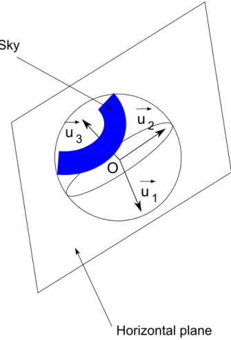
Let °!u1 and °!u2 be the 2 detected directions. A third direction °!u3 can be simply
computed by °!u3 = °!u1£°!u3 or extracted in the image if the scene contains three
main directions. The vectors °!u1, °!u2 and °!u3 permit to define 3 planes, ºijwhich
contain O1, °!ui and °!uj, i 6= j. These 3 planes define 3 diÆerent partitions of
the sphere. The horizontal plane is in fact the plane ºij which partitions the
spherical image without separating points of the sky (Fig8). Let us note that in few cases, it can happen that two ºij planes can be candidate. In this case,
we make a simple tracking of the horizontal plane in the sequence in order to clear up this ambiguity.
Once the horizontal plane has been detected, the vertical direction of the scene is simply the vector °!ui which is not contained in the horizontal plane. This
(a) (b)
(c) (d)
Fig. 7. (a) Original image with the circle of points used for sky detection, (b) binarized histogram of the circle, (c) probable position of the sky with the initial seeds for the region growing (d) detected sky after region growing process
initialization and especially to reset and verify the tracking of the vertical VP. If the sky is not observable (e.g. indoor environment), then we switch to common techniques to detect and track the vertical VP. Experiments to qualitatively measure the accuracy will be performed in section 7.4.
5 Estimation of camera motion between two images
In this section, we aim to estimate the motion between two catadioptric images (fig 9). Let us consider a 3D point M observed by two cameras whose centers are located at C1 and C2 and linked by a rigid transformation (R, T ) where
R 2 SO(3) and T 2 R3, i.e. °°°!C
2M = R.°°°!C1M + T . The spherical projection of
M is noted P 2 S2 for the first image and P0 2 S2 for the second image. P
and P0 are linked by the epipolar constraint:
Fig. 8. The horizontal plane (°!u1, °!u2) partitions the spherical image without
sepa-rating sky points and °!u3 corresponds to the vertical, where °!ui i = 1· · · K represent
the dominant directions of the scene.
Traditional epipolar-based methods, such as essential and fundamental ma-trix (5, 7 and 8-point algorithms) or homography (4-point algorithm) provide a closed-form solution by SVD for the calculation of R and T given a mini-mal number of correspondences. However, as explained in the introduction, it suÆers from several limitations like the di±culty of planar/non-planar scene, the non-computation of R in pure-rotation motion and a high complexity for a robust estimation. To avoid these drawbacks, our approach consists in de-coupling the motion into rotation and translation. In the first part, we explain how to estimate R using the direction of the parallel lines bundles and in the second part, we present our 2-point algorithm for catadioptric vision to estimate T from eq (6).
5.1 Rotation estimation
In section4, we presented a method to compute the absolute attitude (roll and pitch angles). We now present how to compute the complete rotation (i.e. roll, pitch and yaw) from extracted vanishing directions. First, we use a common
Fig. 9. Our goal is to estimate the rotation R and the translation T between two catadioptric images.
technique for the matching of dominant directions in an image sequence. And then we introduce an original method for the computation of R given the correspondences of two directions.
As a first step for rotation estimation, we have to set the correspondences between the detected vanishing directions. A method consists in matching the lines of the bundles (cf [32] for a recent review of existing methods) but it is computationally expensive and thus cannot be used for real-time experi-ments. That is why we preferred using a simple continuity constraint. Let ui
(respectively u0i) be the directions detected in the first image (respectively in the second image) with i = 1, 2,· · · . The continuity constraint simply matches the pair (ui, u0j) having the lowest angle. This method assumes the relative
ro-tation between two images is lower than 45± for the 3 angles. This assumption is valid for video sequences, as will be shown in the experiments section, and moreover, this method has the advantage to be very fast. An important remark is that during a long path, some vanishing points might appear/disappear. In our implementation, we inspired from a method usually applied for robust fea-ture point tracking in SLAM: a VP is added to (reciprocally removed from) the list of VPs when it gets observed (reciprocally not observed) for some frames. A VP is classified as observed (reciprocally not observed) when the number of its associated lines is higher (reciprocally lower) than a certain threshold. This situation is discussed in details in Appendix A.1.
The second step consists in computing the relative rotation given some VP correspondences and we present an original linear method for this task. From the property proven in section 3, the correspondence of two vanishing direc-tions u and u0 in two images verify u0 = Ru where R is the rotation between
inde-pendent equations, which means that two correspondences are su±cient to estimate R. Let u1 and u2 be two dominant directions in the first image, and
their correspondences u0
1 and u02 in the second image. The following relation
holds :
u01 = Ru1 and u02 = Ru2 (7)
Traditionally, this system is non-linear with respect to the three rotation angles roll, pitch and yaw. We propose an original linear method to compute the rotation.
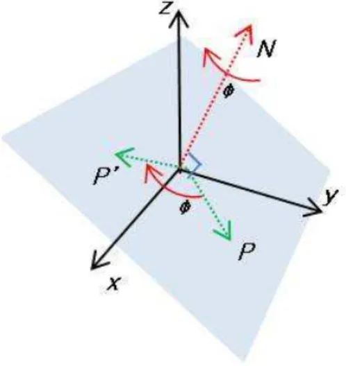
Proposition:
Let us consider a rotation R such that u0
1 = Ru1 and u02 = Ru2, whereku1k =
ku2k = 1. If we decompose R into a rotation axis N and an angle ¡ by
Rodrigues’ formula (cf Fig 10 and eq 8), then N and ¡ can be estimated as follows :
• if u01 = u1 and u02 = u2 (case 1), then R = I and the motion is rotation-free.
• if u0
1 = u1 and u02 6= u2 (case 2), then
N = u1, cos ¡ = u
0
2.u2°(u2.N )2
1°(u2.N )2 and sin ¡ =
u0
2.(N£u2)
kN£u2k2
By symmetry, we obtain the same relations by switching u1 and u2, i.e.
if u01 6= u1 and u02 = u2.
• else (case 3), i.e. u0
1 6= u1 and u02 6= u2, then
N = (u1°u01)£(u2°u02)
k(u1°u01)£(u2°u02)k, cos ¡ =
u0
2.u2°(u2.N )2
1°(u2.N )2 and sin ¡ =
u0
2.(N£u2)
kN£u2k2
Therefore, if two bundles of lines are detected in the images, trivial mathematic operations (cross and dot products) permits to easily retrieve the rotation between the two images.
Proof:
By Rodrigues’ formula, R can be decomposed into a rotation axis N and an angle ¡ as follows:
u0 = Ru
u0 = cos ¡.u + (1° cos ¡)(u.N)N + sin ¡[N £ u]. (8)
To compute R, three cases can occur:
• case 1: obvious
• case 2: if u01 = u1 and u02 6= u2, then u1 is invariant by R and thus N = u1.
Moreover, from eq (8):
therefore
cos ¡ = u02.u2° (u2.N )
2
1° (u2.N )2
In the same way, we obtain
sin ¡ = u02.(N £ u2) kN £ u2k2
.
• case 3: to verify the proposed relation, it su±ces to notice that N is orthog-onal to both (u01 ° u1) and (u02 ° u2). It can be seen by geometry on the
figure10 or by the Rodrigues’ formula (N.(u0
1 ° u1) = N.(u02° u2) = 0)
Fig. 10. Representation of the axis-angle notation for rotation. The point P is ro-tated to the point P0 around an axis N by an angle µ.
5.2 Translation estimation
We are now able to compute the rotation R between two images. What we aim to do now is to calculate the translation T from eq (6). Since T can be known only up to scale, there are only 2 DOF to compute T . As each correspondence provides one equation, two correspondences are su±cient to estimate T . Therefore we name this method the 2-point algorithm.
Let us consider two spherical points Pi and Pj in the first image and their
correspondences P0
i and Pj0 in the second image. From eq (6), we can determine
the translation up to scale by a simple cross-product:
Fig. 11. Geometric interpretation of the 2-point algorithm: each point correspon-dence (note the compensation of the rotation in the first camera) defines an epipolar plane and the intersection of 2 epipolar planes corresponds to the translation.
The geometric interpretation is presented in Fig 11: the translation is the in-tersection of 2 epipolar planes obtained from 2 pairs of point correspondences. One may note that a degeneracy occurs when the points P and P0 are in the direction of the translation. Using 2 non-degenerate correspondences, T can be easily computed by eq (9). For the over-determined case (i.e. K > 2 correspondences are given), eq (9) can be extended as follows:
T = arg min T K X i=1 MiT (10)
where the ith row of M (with i = 1, . . . , K) corresponds to the ith point correspondence: Mi = (RPi £ Pi0)T. The solution T of this system is easily
obtained from the Singular Value Decomposition (SVD) of M . When K = 2 correspondences are given, T can be computed by eq (10) but eq (9) is more recommended due to its much lower computation.
To determine the orientation of T , we simply verify that the “scalar triple product” between RP , P0 and RP £ T is negative, that is to say:
(RP £ P0).(RP £ T ) < 0 (11) Indeed the vectors RP £ P and RP £ T have “an opposite orientation” (cf Appendix A.2).
The direct estimation of T is sensitive to incorrect and noisy matching. Thus it is necessary to use a robust estimation algorithm that can handle point noise and outliers. In [45], the authors review some important robust techniques
and here, we focus on two important ones: M-estimator [8][29] and RANSAC [18]. The principle of the M-estimators is to modify the objective function of the least squares by penalizing the largest residues. On one hand, it can be implemented using a simple iterative re-weighted least squares algorithm, but on the other hand, it requires an initial estimate of the parameters and might not be faster than RANSAC when the data is very noisy. RANSAC approach estimates the considered parameters from a minimal set of data (in our case 2 correspondences), counts the number of data verifying the validity of the estimated parameters and finally retains the best consensus. This method is widely used and very e±cient from the robustness point of view, but is quite time consuming.
In the following, we show that the 2-point algorithm decreases the theoretical complexity of RANSAC, which permits to use it for a fast and robust esti-mation of T . [26] defines the theoretical minimum number of samples that is required to ensure that at least one sample is free from outliers and an exam-ple is depicted by Table1. It clearly shows that the 2-point algorithm requires much less iterations than the 4, 5, 7 or 8-point algorithms, especially when the percentage of outliers is high. Concretely, for 50% of outliers, the number of RANSAC iterations for the 2-point algorithm is 4, 9, 35 and 69 times lower than for the 4, 5, 7 or 8-point algorithms respectively.
Sample size proportion of outliers ≤
s 5% 10% 20% 25% 30% 40% 50% 2 2 3 5 6 7 11 17 4 3 5 9 13 17 34 72 5 4 6 12 17 26 57 146 7 4 8 20 33 54 163 588 8 5 9 26 44 78 272 1177 Table 1
The number of samples required to ensure, with a probability p = 0.99, that at least one sample has no outliers for a given number s of minimal points and a proportion of outliers ≤. s = 2 refers to our approach and s = 4, 5, 7, 8 refers respectively to the 4, 5, 7 and 8-point algorithms. From [26].
6 Relative rotation calibration between a catadioptric camera and a gyroscope
In order to analyze the accuracy of the proposed methods for attitude and rotation estimation, we propose to compare the computed rotation angles with ground truth data obtained by a gyroscope rigidly attached to the camera.
Fig. 12. The coordinate systems of the camera and the gyroscope
The gyroscope returns the orientation between its own frame and an Earth coordinate system composed of magnetic North, West and opposite gravity directions. On the contrary, our method computes the orientation between the vanishing directions detected in an image pair. That is why the results obtained from these two sensors cannot be directly compared. In order to calibrate an Inertial Measurement Unit (IMU) with a camera, [40] estimates the relative rotation by having both sensors observing the vertical direction at diÆerent poses (fig 12). Vertical is obtained from the camera by using a chessboard target and from the IMU by magnetic field information. However our gyroscope only provides absolute angles and thus this method cannot be directly applied. Nevertheless, the knowledge of the orientation angles (Ω, √, Æ) permits to recompute the vertical direction °!N = (nx, ny, nz) in the gyroscope
frame by the relation defined in eq (4).
The vertical direction in the image could be computed from a specific target (e.g. line pattern), but it is not very convenient. We preferred to run the algorithm presented in sections 2.3 and 3.2 and select the vertical among the detected directions. In theory, such a procedure would also be possible for conventional cameras but in practice, it is complicated because of the limited number of observable lines, the sensitivity to measurement noise and the fact that the vanishing points do not lie inside the image. Given the vertical direction in the gyroscope and camera frames, we simply have to find the unit quaternion ˙q that maximizes:
n X i=1
( ˙qNi˙q§)· Vi (12)
where Vi and Ni respectively represent the vertical in the camera and the
gyroscope frames and n is the number of images. This system is easily solved by [28] and permits to obtain the calibration rotation matrix Rcalib.
7 Experimental results
This section presents some important experimental results concerning the methods that we have proposed in this paper. First, we perform the rela-tive rotation calibration between a catadioptric camera and a gyroscope. The obtained alignment correctly corresponds to the layout of our system. Then, we qualitatively measure the accuracy of the proposed attitude estimation and obtain a mean error of 2.5± and 3.5± degrees for the roll and pitch
an-gles. Experiments also prove the inherent non-accumulation of error. Finally, we measure the performance of the 2-point algorithm on synthesized and real data. Tests have proved that the 2-point algorithm is more robust and accu-rate than essential matrix and homography, even if the rotation information is noised.
7.1 Equipment
Two catadioptric systems have been used for the experiments. The first one is composed of a paraboloid mirror manufactured by Panosmart and a Sony DFW-SX910 camera. The second system combines a mirror made by the com-pany 0-360 and a Canon PowerShot G10. The image resolutions are 1024x768 for the section 7.4 of rotation estimation and 1280x960 for the motion esti-mation. To calibrate the catadioptric system, we have used the toolbox based on [4] and available on Internet. The ground truth rotation data have been acquired from the Xsens MTi.
7.2 Line extraction
This section aims to demonstrate the advantages of our line detection ap-proach: general, fast, accurate and robust. By construction, it is obvious that our method is general in the sense that it can deal with any central cata-dioptric cameras (equivalent sphere). In order to study the execution time, we have implemented our method in C++ using OpenCV library. We are able to detect lines in less than 30 ms (about 34 fps) for 1280x960 images with non-optimized code. Therefore our method can be used for real-time systems. Then we analyze the robustness and accuracy aspects. First we study the de-pendance to edge pixel noise and we apply the following procedure: generate 1000 synthesized catadioptric images containing the projection of one random line, add gaussian noise with zero mean and an increasing standard deviation (from 0 to 5 pixels) and apply the proposed split-and-merge algorithm. The error is defined as the angle in degrees between the detected and the true
(a) (b)
Fig. 13. Typical results of line detection on noisy data. (a): line detection results after splitting step. The green dots corresponds to the noisy data points and the red conics to the extracted lines. (b): line detection results after merging step and imposing only one line.
(a) (b)
Fig. 14. Mean (a) and standard deviation (b) of the angular error in degrees (y-axis) with respect to standard deviation of noise on edge pixels (from 0 to 5 pixels on x-axis)
normals: for perfect detection, error is 0± and in the worst case error is 90±.
In case of very strong noise, our algorithm might not merge all the detected normals, so we force to use all the data points in order to get only one normal vector (cf Fig 13 for intermediate results). Results are presented in Fig 14. As expected, the error increases when the noise standard deviation increases. The important fact to notice is that even with a very high standard deviation of 5 pixels, the mean error is less than 1±. Secondly, we study the dependance
to conic occlusion (Fig 15). For this, we extracted one arc of a specific max-imum amplitude from the displayed conic (from 0± to 358±), then added a gaussian noise with mean=0 and std=2 pixels on the edge pixels and finally applied the previous procedure (i.e. split-and-merge algorithm and mean of detected normals). Results of Fig 16 confirm the intuitive idea according to which the error becomes higher when the conic occlusion increases (inversely conic amplitude decreases). It is worthwhile noting that even for a very high
(a) (b)
Fig. 15. Typical results of line detection on noisy data (mean=0, std=2 pixels) and very high occlusion (350±). For information, the error is 2.18± for (a) and 4.55± for
(b).
(a) (b)
Fig. 16. Mean (a) and standard deviation (b) of the angular error in degrees (y-axis) with respect to conic occlusion (from 0± to 358± on x-axis) with an additional noise
of std=2 pixels on edge pixels
(a) (b)
Fig. 17. EÆect of the merging step on the line detection accuracy. Same legend than 16.
Fig. 18. Observation of the vertical direction (vx, vy, vz in the y-axis) from the
gyroscope (left) and the catadioptric camera (right) along 520 frames (x-axis). One may notice the relationship between these two sensors: a near 180± rotation about
the camera z-axis.
occlusion of 350±, the mean error is less than 0.3±. Thirdly, we study the eÆect
of the merging step. Due to occlusion, some lines can be separated into sev-eral parts during the chaining step. The merging step is going to re-associate these parts. Since more parts will be used, the occlusion will be smaller and the fitting more accurate, especially when occlusion is high. For validation, we compare the accuracy of line detection with and without the merging step. Results are depicted in Fig17and confirm this intuitive idea. As a conclusion, these experimental results demonstrate the robustness and accuracy of our proposed method.
7.3 Camera-gyroscope rotation calibration
As explained in section 6, the camera-gyroscope rotation calibration is based on the vertical directions observed from the gyroscope and the camera. The vertical in the gyroscope frame was computed by reading the orientation an-gles and applying eq (4). To obtain the vertical direction in the camera frame, we have detected the dominant directions in the images, manually selected the vertical for the first frame, and finally tracked it during a video sequence. Figure 18 depicts these measurements. The quaternion obtained by [28] cor-responds to the following relative angles: roll = °2.82±, pitch = 0.01± and
yaw = °179.1±, i.e. a near 180± rotation about the camera z-axis, which is
consistent to the layout of our system. Comparing the gyroscope vertical with the newly calibrated camera vertical, we have obtained a mean error of 2.0±
7.4 Rotation estimation
The robustness of the method strongly depends on the number of catadioptric lines available in the scene and on the quality of their extraction. Since we have shown that our method of catadioptric line extraction is particularly robust to noise and occlusion (cf section7.2), the single real constraint deals with the possibility to detect at least two bundles of parallel lines. Since it is necessary to detect at least three lines for each bundle, the presence of two sets of three parallel lines is su±cient for our algorithm to estimate the complete rotation.
(a) (b)
(c) (d)
Fig. 19. Detection of the 2 dominant vanishing points and their associated parallel lines. Each conic represents a detected line and its color corresponds to the set of parallel lines it belongs to. It shows that the vanishing points can be robustly extracted and continuously tracked along the whole sequence despite large camera motion.
To analyze our method for rotation estimation, we have acquired a video sequence composed of 520 frames at 2 frames per second and the associated gyroscope data. The video was acquired in a parking lot of our university (i.e. a typical urban scene). The total travel path is about 40 meters and the rotation amplitude is about 40± for roll, 60± for pitch and 360± for yaw angles. Figure
19depicts typical results of vanishing points extraction for this sequence and Fig 20 compares the evolution of the roll, pitch and yaw angles obtained by
Fig. 20. Comparison of roll (top), pitch (middle) and yaw (bottom) angles between gyroscope (red dashed line) and the proposed method (blue solid line). The “jumps” of the yaw angle are simply due to the discontinuities (-180±,+180±).
the gyroscope and our approach. The mean errors for the 3 angles are 1.2±, 1.3± and 3.9±, which proves the accuracy of our method. One may also note
that the evolution of the angles is very smooth whereas no filtering technique has been used.
7.5 Motion estimation
This part analyzes the accuracy and the robustness of the 2-point algorithm. First, we perform some experiments on synthesized data to study its depen-dency to noised matching points and inaccurate rotation estimation. Then we apply the algorithm on real indoor and outdoor sequences.
7.5.1 Synthesized data Noise dependency
To analyze the dependency of our 2-point algorithm to data noise, we synthe-sized 1000 catadioptric images composed of 100 matching points and we have applied to their coordinates a gaussian noise of mean=0 and std=1pixel and 3pixels. In a first series of experiments, the ground truth rotation was directly used for the computation of T by the 2-point algorithm. To simulate the fact that the rotation cannot be perfectly estimated from the images, we have per-formed a second series of experiments where the 3 rotation angles have been
(a) (b)
(c) (d)
Fig. 21. Comparison of mean (left column) and std (right column) error in degrees (y axis) for the estimation of the translation direction on synthesized catadioptric images by the 5-point and the proposed 2-point algorithm, with respect to rotation noise (mean=0 and increasing std on x-axis in degrees). On top row, data points have been noised by a gaussian distribution of mean=0 and std=1pixel; on bottom row, std=3pixels. It clearly shows that the 2-point algorithm is more reliable that the 5-point method up to a certain level of rotation noise, especially when the data noise increases.
corrupted by a gaussian noise of mean=0 and an increasing std=[0±, . . . , 2±].
For comparison, we have also applied the state-of-the-art 5-point algorithm to compute the essential matrix [50]. Figure 21depicts the mean/std error in degrees for the estimation of the translation direction. The std noise for data points is 1± for top row and 3± for bottom row. As the 5-point algorithm and
the 2-point algorithm with true rotation do not depend on the rotation noise, their error is constant. It can be noticed that the error of the 2-point algorithm with noised rotation linearly increases with the level of rotation noise but that it performs better than the state-of-the-art 5-point algorithm up to a certain level of rotation noise. It shows that the 2-point algorithm is more e±cient than the 5-point algorithm even when the rotation is corrupted by an accept-able level of noise, especially when the noise of data points increases. It is a very important result because it demonstrates that the constraint provided by the rotation and the fact that only 2 points are required permits to obtain a
more robust estimation by the proposed method.
Fig. 22. Comparison of execution time (note the y-axis scale, base unit for the 2-point method) for the translation estimation by the 2 (our), 4, 5, 7 and 8-point algorithms for a single RANSAC iteration. Refer to text for more details.
Computation time
In this section, we want to demonstrate that the translation estimation by our 2-point algorithm is faster than by commonly used techniques: 4, 5, 7 and 8-point algorithms. For the implementation of the 4, 7 and 8-point algorithms, we referred to [26]. For the 5-point algorithm, we based our implementation
Fig. 23. Comparison of execution time (in ms with a logarithmic scale) for the translation estimation by the 2 (our), 4, 5, 7 and 8-point algorithms for the minimum number of theoretical RANSAC iterations with an increasing percentage of outliers from 5% to 50% . Refer to text for more details.
on [50]. Therefore, in this section about synthesized data, the execution time of RANSAC iteration contains only the computation of the associated matrix (T for 2-point by eq (9), H for 4-point, E for 5-point and F for 7 and 8-point algorithms). For generality purpose and fair comparison, this execution time does not contain the count of the number of consistent inliers because it depends on the synthesized points (e.g. E matrix obtained by the 5-point algorithm can have between 1 and 10 solutions and F obtained by the 7-point algorithm between 1 and 3) and especially the robust procedure which is used (e.g. preemptive RANSAC [49], Td.d-test-RANSAC [11] or RANSAC
with SPRT [12]). Figure 22 compares the average execution time for a single RANSAC iteration. It shows that the translation estimation by the proposed eq (9) is at the order of 200, 900, 250 and 300 faster than the 4, 5, 7 and 8-point algorithms respectively. It can be noticed that the 5-point algorithm is at least 3 times slower than any other algorithms because it requires several extensive computations: matrix nullspace, Gauss-Jordan elimination, roots of a tenth degree polynomial, etc. Figure23compares the average execution time to compute the associated matrices for the minimum number of theoretical RANSAC iterations, as listed in Table 1, with an increasing percentage of outliers. It shows that our proposed 2-point algorithm is drastically faster than the commonly used techniques, at the order of 800, 7800, 860 and 2000 compared to the 4, 5, 7 and 8-point algorithms respectively for 50% of outliers. Section on real data will compare the execution time of the entire RANSAC procedure (computation of the associated matrix and count of the number of inliers).
7.5.2 Indoor sequence
In this experiment, we aim to estimate the camera trajectory for an indoor se-quence. This sequence is composed of 33 images taken in pure translation with an interval of 30cm to 50cm between each acquisition (Fig. 24). Pure trans-lation was preferred simply because it simplifies the measurement of ground truth motion. .
Before computing the motion, we have to choose a method for features extrac-tion and matching. Because of the distorextrac-tions introduced by the mirror, the analysis of omnidirectional images needs adapted tools [14][24]. However these methods increase the execution time significantly. Indeed they impose a reg-ular sampling of the spherical image and require image interpolation. That is why we cannot use this kind of techniques. As we need a few correspondences (at least 2) between the images, a classical method of point feature matching is su±cient. Thus we have simply used SIFT [41]. Even if this method is not theoretically appropriate to omnidirectional images, experimental results have shown a very good robustness.
Whereas it is known there is almost no rotation in our indoor sequence, we have applied our rotation estimation algorithm to show that our method can handle this situation correctly. Then we have estimated the translation using the 2-point algorithm of section 5.2. Let (Pi, Pi0), i = 1· · · N be N points
matched between two images and ni = RPi£ Pi0. Each vector ni define a great
circle Ci (fig 4) and equation (9) means that all these great circles intersect in
two antipodal points I1, I2 2 S2 and that I1I2 ª T .
(a) (b)
Fig. 24. (a) great circles Ci (red curves) defined from the matching of N feature
points (green dots) between two images of the indoor sequence (b) great circles defined as inliers by RANSAC. Great circles and feature points have been enlarged for a better visualization.
Figure 24shows the translation estimation between two consecutive images of the sequence. On Fig 24(a), we project the great circles Ci of the N matched
points in the catadioptric images. As these circles do not intersect in the same points, we can notice several incorrect features matchings. RANSAC permits to solve this problem and detect the outliers (Fig.24(b)). To compute the camera trajectory, we composed the estimated motions estimated at each frame. Formally, let (Rk, Tk) be the rotation and translation between Ck°1 and
Ck, where Ci is the camera location of the i + 1th image. The camera location
(xk, yk, zk) at Ck is computed by composition: 0 B B B B B B B B @ xk yk zk 1 1 C C C C C C C C A = (PkPk°1· · · P1)°1 0 B B B B B B B B @ 0 0 0 1 1 C C C C C C C C A = 0 B @ 0 B @ Rk Tk 03£3 1 1 C A 0 B @Rk°1 Tk°1 03£3 1 1 C A· · · 0 B @ R1 T1 03£3 1 1 C A 1 C A °10 B @03£1 1 1 C A (13)
camera. Figure 25 shows the estimated camera motion using the proposed method, which is consistent with the rectilinear ground truth motion.
(a) (b)
(c)
Fig. 25. Motion estimation for the indoor sequence: 3D view (a), top-view (b) and side-view (c).
7.5.3 Outdoor sequence
This section presents the results of our method in outdoor environment. This outdoor sequence is composed of 72 frames with an interval of 50-70 cm and the camera moves along a rough rectilinear path. However, we do not know the exact trajectory. Figure 26 depicts the extraction of vanishing points for rotation estimation in this outdoor sequence. Figure27shows the evolution of the camera’s 3D position along the sequence. In the top-view, the estimated trajectory follows the rough rectilinear path. In the side-view, the altitude seems to decrease. It is simply due to the fact that the trajectory is expressed with respect to the coordinate system of the first camera which is not aligned with the vertical. An interesting fact is that the estimated altitude is linear, which means the camera’s height is constant. This result is consistent with the experiment since the camera was attached on a tripod with a fixed height. Figure28compares the execution time for the minimum number of theoretical RANSAC iterations for 50% of outliers. This execution time contains the entire RANSAC process: random selection of the N required correspondences, the computation of the associated matrix (T for 2-point, H for 4-point, E for 5-point and F for 7 and 8-point algorithm) and also the count of the number of consistent inliers. This graph clearly shows that our proposed method is greatly faster than traditional 4, 5, 7 and 8-point algorithms and runs in real-time. It is also interesting to note that figure 22showed that computing F by
(a) (b)
Fig. 26. Rotation estimation for the outdoor sequence by vanishing point extraction. Same legend than figure 19.
(a) (b)
(c)
Fig. 27. Motion estimation for the outdoor sequence: 3D view (a), side-view (b) and top-view (c).
the 8-point algorithm is faster than computing E by the 5-point algorithm, but in figure 28 the complete RANSAC procedure is slower for the 8-point than for the 5-point algorithm. This is due to the fact that the 8-point algorithm requires much more RANSAC iterations to ensure that at least one sample has no outliers (cf Table 1). On the contrary, the proposed 2-point algorithm is not only the fastest to compute T but also requires the lowest number of RANSAC iterations.
8 Conclusion
In this paper we have presented a new approach for estimating egomotion in man-made environments by catadioptric vision. The main idea consists in
Fig. 28. Comparison of execution time in ms (y-axis), in each frame of the sequence, for the translation estimation by the 2 (our), 4, 5, 7 and 8-point algorithms using the minimum number of theoretical RANSAC iterations for 50% outliers and applied for the real outdoor sequence. Refer to text for more details.
decoupling the motion into rotation and translation. The proposed method for rotation estimation is based on our new line detection algorithm for cata-dioptric images. We have experimentally demonstrated that extracting lines and the associated vanishing points can be performed in real-time, and is accurate and robust to both noise and occlusion. Using line information, we have also introduced a method that is able to explicitly estimate the absolute attitude (roll and pitch angles) without error accumulation. It requires the vertical direction in the image and we have proposed an original algorithm that can automatically select or compute the vertical from the detected van-ishing directions. Comparison of attitude estimation with ground truth data demonstrated the accuracy of our method and the inherent non-accumulation of error.
Concerning translation estimation, we have introduced a 2-point algorithm for catadioptric vision. This method oÆers many advantages compared to other existing methods. First, it can implicitly handle diÆerent scene geometries (planar/non-planar) contrary to essential/fundamental matrix and homogra-phy, and thus does not need complicated switching mechanism between E/F and H. Second, the translation estimation is more robust to noised corre-spondences thanks to the constraint provided by the rotation. Thus it can handle not only small displacements but also large rotations and translations. The third advantage is the fast execution. The fact that only 2 points are re-quired permits to greatly reduce the number of rere-quired RANSAC iterations to guarantee that at least one sample is free from outliers. We have shown that the 2-point algorithm requires 4, 9, 35 and 69 times less RANSAC iter-ations than the 4, 5, 7 and 8-point algorithms for 50% of outliers, speeding up the RANSAC procedure by at least these orders of comparison. More-over 3 simple cross-products permit to compute the translation contrary to