Speckle noise spectrum at near-nadir incidence angles for a time-varying sea surface

HAL Id: insu-03008365

https://hal-insu.archives-ouvertes.fr/insu-03008365

Submitted on 16 Nov 2020

HAL is a multi-disciplinary open access

archive for the deposit and dissemination of

sci-entific research documents, whether they are

pub-lished or not. The documents may come from

teaching and research institutions in France or

abroad, or from public or private research centers.

L’archive ouverte pluridisciplinaire HAL, est

destinée au dépôt et à la diffusion de documents

scientifiques de niveau recherche, publiés ou non,

émanant des établissements d’enseignement et de

recherche français ou étrangers, des laboratoires

publics ou privés.

Speckle noise spectrum at near-nadir incidence angles

for a time-varying sea surface

Ping Chen, Danièle Hauser, Shihao Zou, Jianyang Si, Eva Le Merle

To cite this version:

Ping Chen, Danièle Hauser, Shihao Zou, Jianyang Si, Eva Le Merle.

Speckle noise

spec-trum at near-nadir incidence angles for a time-varying sea surface. IEEE Transactions on

Geo-science and Remote Sensing, Institute of Electrical and Electronics Engineers, 2020, (in press).

�10.1109/TGRS.2020.3037910�. �insu-03008365�

Speckle noise spectrum at near-nadir incidence angles

for a time-varying sea surface

Ping Chen, Danièle Hauser, IEEE Member, Shihao Zou, Jianyang Si, Eva Le Merle

Abstract—Speckle noise is inherent to radar measurements. For

applications which need both a high temporal and high spatial resolution, a classical method for the reduction of the speckle noise by filtering the backscattered signal may not be sufficient. In particular, when radar observations are used to estimate ocean wave spectra from relative fluctuations of the radar signal within a given footprint, a method must be implemented to correct for the speckle effect in the Fourier domain (i.e. density spectrum). A theoretical background to model the speckle density spectrum for a radar with near-nadir incidences was proposed by Jackson in 1981 but it is based on a stationary sea surface assumption and ignores the variation of the main factor in the four-frequency moment near the origin. In this paper, we revisit this theoretical background to extend this model to a time-varying sea surface and alleviate some assumptions on the Fresnel phase formulation. The results from the model applied in the configuration of an airborne system indicate that not only the displacement of the radar but also the dynamic properties of the sea surfaces have a significant effect on the speckle noise spectrum in certain directions of observations. The effects depend on the radar look direction in azimuth, and on sea surface conditions (wind speed, wind direction with respect to the aircraft route, surface wave spectrum). This new model is validated against observations of the airborne near-nadir incidence scatterometer –KuROS. We show in particular that the errors between the experimental estimation of the omni-directional speckle noise spectrum from KuROS and the prediction by our model are below 10%.

Index Terms—speckle noise spectrum, time-varying sea surface,

near-nadir incidence, Geometry Optical approximation I. INTRODUCTION

Speckle noise is inherent to radar measurements used to sense geophysical media composed of distributed scattering elements (e. g., sea surface). Indeed, the composite backscatter generated by these media is the coherent sum of components backscattered from individual elements which generate different phases and amplitudes, and add together to give a resultant whose intensity varies randomly. Thus, the backscattered signal measured by a radar exhibits fluctuations from one look to the next one, even when the surface is the same. When radar systems are used to estimate ocean wave properties from the analysis of signal fluctuations at a relatively high spatial resolution (typically 5 to 30 m horizontally), the speckle noise is a perturbing effect which must be accounted for in the inversion of the fluctuation spectra into wave spectra [1], [2], [3], [4].

There are presently two main categories of radar systems

devoted to the measurement of ocean wave spectra: those based on a SAR side-looking configuration (see e.g. [2], [5], [6], [7], [8]), and those based on a RAR real-aperture and azimuthally scanning configuration [9], [10]. In both cases the spectrum of ocean waves is derived from the spectra of signal fluctuations analyzed over a footprint of several kilometers. In both cases, it requires to subtract the speckle noise spectrum from the fluctuation spectrum.

Jackson provided the theoretical background to model the speckle noise contribution in the Fourier domain (spectrum of signal fluctuations in space and time) for a real-aperture near-nadir looking radar [1]. Based on this theoretical approach, a simple formula was then proposed to represent the speckle density spectrum as a function of the wave number at the surface [11]. Later, Hauser proposed an empirical method to derive the parameters of the Jackson’s model speckle spectrum from airborne observations with a scanning real-aperture radar [3]. It consists in estimating a mean spectrum of speckle from a combination of fluctuation spectra obtained with radar signals integrated over different durations. This speckle spectrum is then subtracted from the fluctuation spectrum to estimate the modulation spectrum due to waves.

Engen and Johnsen proposed another method the so-called “cross-spectrum” method to remove the speckle noise contribution from SAR observations over the ocean using successive looks [2]. It is based on the conjugate product of successive fluctuation spectra obtained from overlapping scenes. This method is now operationally used by The European Space Agency to provide wave spectra from SAR images. It was also later used by Caudal [10] and Le Merle [12] in the processing of their airborne real-aperture scanning radar observations to retrieve wave spectra.

Both empirical methods (based on cross-spectra or on multi-duration time integration) are very efficient but are constrained by the conditions of measurements (appropriate overlap of successive looks). With the recent launch of the CFOSAT satellite and its real-aperture wave spectrometer SWIM in operation, the question of speckle estimation is still of actuality, because the SWIM mode of operation is not well appropriate neither to the cross-spectral method (limited overlap of successive scenes in the nominal mode of acquisition) nor to the multi-integration method (loss of range resolution in this case). Therefore, an empirical ad’hoc speckle model was estimated from the SWIM observations [4] and is currently used to invert the wave spectra from the fluctuation spectra. The results indicate that this empirical speckle spectrum shows an important increase in a sector of ±15° and that its level depends on azimuth with respect to the flight-track, on latitude, and on sea-surface conditions.

Although all the proposed empirical methods to estimate or subtract the speckle noise spectrum are convenient from an operational point of view, they are still difficult to reconcile with the existing theoretical background. Therefore, in the present study we propose to revisit the analytical model of Jackson of speckle noise spectrum.

Jackson established an analytical speckle noise spectrum model based on the Geometry Optical approximation for the Manuscript received September 04, 2020; accepted October 26, 2020. This

work was supported in part by the National Key Research and Development Program of China (2016YFC1401005), the National Natural Science Foundation of China under Grant 41976168, Grant 41976173, and Shandong Provincial Natural Science Foundation of China under Grant ZR2019MD016. (Corresponding author: Ping Chen.)

Ping Chen, Shihao Zou, and Jianyang Si are with the School of Electronic Information and Communications, Huazhong University of Science and Technology, Wuhan, 430074, China (e-mail:chenping@hust.edu.cn; zoushshawn@163.com;m201972058@hust.edu.cn).

Danièle Hauser, and Eva Le Merle are with the LATMOS, Université Paris-Saclay, UVSQ, CNRS, Sorbonne Université, 78280 Guyancourt, France(email:daniele.hauser@latmos.ipsl.fr ;eva.lemerle@latmos.ipsl.fr) .

scattering processes expressed for a frozen sea surface [1], a pulse-limited transmitted waveform with a given range resolution and integration time. This model takes into account the displacement of the illuminated ocean scene with respect to the radar in an azimuthal scanning geometry, but it does not take into account the surface scatter motion. The consequence is that, according to this model, the speckle noise spectrum along the flight direction tends to very large values because the number of independent samples forming the integrated radar echo is supposed to tend to one. However, this is in contradiction with the actual situation as seen from both airborne and spaceborne observations, which indicate that in spite of an important increase of speckle when the radar look direction is approximatively aligned with the platform displacement the number of independent samples deduced from the speckle noise spectrum is far more than 1.

We will demonstrate in this paper that this is because in certain conditions, the kinematic properties of the sea surface cannot be ignored. Indeed, during the radar integration time (several tens micro-seconds typically), the correlation time of the scattered field from the sea surface cannot be ignored, since it is typically a few milliseconds [13].

Jackson proposed a simplified analytical expression of his model of speckle spectrum under the assumption of a Gaussian shaped transmitted wave form [11]. However, because the dynamic properties of the sea surface were ignored, the speckle noise spectrum density along the flight direction estimated from this modified model is still much larger than the one measured. Up to now there is no analytical model of speckle noise spectrum in which both the radar motion and time-varying properties of the sea surface are taken into account.

This is precisely the aim of this paper to propose an analytical noise spectrum model valid for a radar with near-nadir incidences, and a time-varying sea surface. There are two differences compared with Jackson's initial publication [1]. The first is that in addition to the movement of the radar, we take into account the kinematic properties of sea surface during the radar integration time. The second is that in our approach, we remove the assumption used in Jackson’s model that the variation of the main factor in the four-frequency moment of the surface scattering matrix near the origin tends to zero. Furthermore, we propose here a validation of the model by using independent speckle spectrum estimates from observations.

In Section II, the speckle spectrum model for a time-varying sea surface is presented with the movements of both radar and sea surface scatters taken into account. In Section III, we present results obtained with this model and a prescribed sea state (imposing a surface wave height and wind) for different sea-surface conditions and for a radar configuration corresponding to airborne observations. In section IV, we present empirical estimates of the speckle noise spectrum obtained from the airborne real-aperture azimuthally scanning KuROS radar [4]. In section V, we compare the speckle spectra predicted by the model to those estimated directly from the KuROS observations. In section VI, we extend our analysis of the model results to other configurations of observations (other radar frequency, platform speed, incidence angles, footprint dimension). Conclusion and perspectives are drawn in section VII.

II. MODEL OF SPECKLE NOISE SPECTRUM FOR AN OCEAN WAVE SCATTEROMETER OVER A

MOVING SURFACE

Jackson expressed the ensemble average fluctuation spectrum of the signal as a function of frequency ω as:

P̃(ω) = ∭ 𝑊(Ω0− 𝐾⃗⃗ ⋅ 𝑉⃗ )N(ν, ν′, ω, Ω0)𝐸0(ν) ∙

𝐸0∗(ν − 𝜔) ∙ 𝐸0∗(ν′) ∙ 𝐸0(ν′− 𝜔)𝑑Ω0𝑑ν𝑑 (1)

where 𝐸0(ν) is the Fourier Transform (FT) of the incident

short-pulsed waveform, 𝑊 is the filter window associated to the integration of the signal over an integral time 𝑇𝑖𝑛𝑡 ,

N(ν, ν′_{, ω, Ω}

0) is the FT of the ‘four-frequency’ moment of the

surface scattering function (see below), 𝐾⃗⃗ ⋅ 𝑉⃗ is the Doppler frequency induced by the platform motion 𝑉⃗ , 𝐾⃗⃗ the wavenumber at the surface, and the asterisk denotes complex conjugate. Expressions of these terms are given in [1] and recalled below: 𝑊(Ω0) = [ sin(Ω0⋅𝑇𝑖𝑛𝑡₂ ) Ω₀⋅𝑇𝑖𝑛𝑡₂ ] 2 (2) 𝑁(𝜈, 𝜈′_{, 𝜔, Ω} 0) = ∫_2𝜋1 𝑀(𝜈, 𝜈′, 𝜔, ∆𝑡) 𝑒𝑥𝑝 (𝑖Ω0∆𝑡) 𝑑∆𝑡 (3) 𝑀(𝜈, 𝜈′_{, 𝜔, ∆𝑡) =< 𝑆(𝜈, 𝑡) ∙ 𝑆}∗_{(𝜈 − 𝜔, 𝑡) ∙ 𝑆}∗_(𝜈′_{, 𝑡 + ∆𝑡)} ∙ 𝑆(𝜈′_{− 𝜔, 𝑡 + ∆𝑡) > (4)}

𝑀(ν, ν′_{, ω, ∆𝑡) is a four-frequency moment defined from the}

surface scattering transfer function 𝑆(ν, 𝑡), where 𝑡 is the ‘slow time’ in the radar chronogram, ν, ν′ _{are the angular frequency}

of the electromagnetic wave, ω is the angular frequency difference, ∆𝑡 is the time interval (the full list of symbols is given in Appendix B).

Equation (1-4) here above are identical to (7-12) in [1]. Jackson then transposes this formalism to the wavenumber domain by writing, ν = 𝑘𝑐 , ν′_{= 𝑘}′_{𝑐 , 𝜔 = 𝜅𝑐 , ∆ν = ν −}

ν′ _{, ∆𝑘 = 𝑘 − 𝑘}′ _{, 𝐾⃗⃗ = 2𝜅𝑠𝑖𝑛𝜃𝜌 , ∆𝐾 = 2∆𝑘𝑠𝑖𝑛𝜃 , where 𝑐 is}

the light speed, 𝜌 is the unit vector of the range direction of the radar, and 𝜃 the incidence angle.

Then, 𝑆(ν, 𝑡) is developed using the geometrical optics scattering approximation which is valid at near-nadir incidence angles [14]. Assuming a Gaussian shape of the transmitted pulse and a Gaussian pattern for the antenna beam, Jackson finally obtains the spectrum of the signal (integrated over 𝑇𝑖𝑛𝑡)

in wavenumber as the sum of two terms [1], [11], one associated with fluctuations due to the long detected waves (through their tilting impact on the backscattered signal) and the other one with the fading (speckle) noise.

Considering a more realistic shape of the transmitted pulse, namely a sinus cardinal function 𝑒0(𝑥) = 𝑠𝑖𝑛𝑐 (_𝛿𝑥𝑥) , with

𝛿𝑥 =_{2𝐵𝑠𝑖𝑛𝜃}𝑐 , where B is the bandwidth of the transmitted pulse, and 𝑠𝑖𝑛𝑐(𝑥) =sin(𝜋𝑥)_𝜋𝑥 , with x is the horizontal range along the range direction 𝜌 of the radar, then the speckle noise spectrum of Jackson’s model when applied to the relative fluctuations of the backscattering coefficient becomes:

P𝑠𝑝_𝐽𝑎𝑐(𝐾, Φ) = 𝑡𝑟𝑖 (_2𝜋𝐾𝐾

𝑝)

1

2𝜋𝐾_𝑝𝑁_𝐽𝑎𝑐(Φ) (5a)

where tri is the triangle function, K is the wavenumber at the surface, Φ is the azimuth angle relative to the flight direction, 𝐾𝑝=_𝛿𝑥1 =2𝐵𝑠𝑖𝑛𝜃_𝑐 (5b)

𝑁𝐽𝑎𝑐 is the number of independent samples due to the radar

displacement:

𝑁𝐽𝑎𝑐(Φ) = 𝑇𝑖𝑛𝑡2𝑉_𝜆 𝛽𝜙sinΦ (5c)

where 𝛽𝜙 is the one-way antenna aperture in azimuth, 𝑉 the

platform speed and 𝜆 the radar wavelength.

Firstly, the sea surface is assumed frozen over the 𝑇𝑖𝑛𝑡 duration:

the sea surface height of a point 𝑥 on the surface is expressed as ξ(𝑥 ). This is a strong assumption. Indeed, for ocean wave scatterometer, the value of 𝑇𝑖𝑛𝑡 is the order of ten microseconds,

typically 30 to 40ms for SWIM [4], 33ms for KuROS [10]. However, at Ku band, the correlation time of the electro-magnetic field scattered by the sea surface is expected to be of the order of millisecond [13]. Thus, the dynamic properties of the sea surface should be taken into account during the 𝑇𝑖𝑛𝑡

duration. Especially, when the observation azimuth angle is close to the flight direction, the number of independent samples induced by the movement of the platform (𝑁𝐽𝑎𝑐) is close to one,

so that the number of actual independent samples is mainly determined by the movement of the sea surface scatters. Thus, for radar observations obtained with an azimuthally scanning system, besides the movement of the radar, the instantaneous velocity of the sea surface scatters must be included in a model of speckle noise spectrum. The second hypothesis by Jackson is that the variation of the main factor in the four-frequency moment near the origin tends to 0 [1]. This assumption simplifies the derivation greatly, but its validity needs to be assessed.

Note also that Jackson, added a coefficient (1+𝜇) in (5) [11], to account for the variation of speckle noise on the signal modulated by the tilting waves:

P′𝑠𝑝_𝐽𝑎𝑐(𝐾, Φ) = 𝑡𝑟𝑖 (_2𝜋𝐾𝐾 𝑝) 1 2𝜋𝐾_𝑝𝑁′_𝐽𝑎𝑐(Φ) (6a) 𝑁′ 𝐽𝑎𝑐(Φ) = 𝑁𝐽𝑎𝑐(Φ)/(1 + 𝜇) (6b) 𝜇 = ∫ 𝑃𝑚𝑜𝑑(𝐾, Φ)𝑑𝐾 (7)

where 𝑃𝑚𝑜𝑑 is the spectrum of the relative fluctuations due to

the presence of long waves.

However, the effect of 𝑃𝑚𝑜𝑑 on the speckle is accounted for

in our model by another way, as explained below and in the appendix.

In order to extend Jackson’s speckle noise spectrum theory to a time-varying sea surface, we expressed the surface elevation as a time and space variable ξ(𝑥 , 𝑡) . Substituting ξ(𝑥 , 𝑡)into the surface scattering transfer function 𝑆(𝑣, 𝑡), and assuming the sea surface to be stationary in the mean and ergodic, then applying Longuest-Higgins’ method [15] to expand the bracket term < ⋯ > in four-frequency moment 𝑀(𝑣, 𝑣′_{, 𝜔, ∆𝑡) and calculating four integrations about all 𝑥}

𝑖

⃗⃗⃗ , i=1,2,3,4, the fluctuation spectrum equation for a time-varying sea surface is obtained (See Appendix A for details). Accordingly, the new speckle noise spectrum model is

P𝑠𝑝(𝐾, Φ) = 𝑡𝑟𝑖 (_2𝜋𝐾𝐾 𝑝) 1 2𝜋𝐾_𝑝𝑁_𝑡𝑜𝑡(Φ) (8a) Where _𝑁1 𝑡𝑜𝑡= 1 𝑁_𝑚𝑜𝑣+ 1 𝑁_𝑖𝑛𝑡, (8b) 𝑁𝑚𝑜𝑣(𝛷) = √𝑁𝑝𝑙𝑎𝑡𝑓2 + 𝑁𝑠𝑢𝑟𝑓2 , (8c) 𝑁𝑝𝑙𝑎𝑡𝑓(𝛷) = 𝑁𝐽𝑎𝑐(𝛷), (8d) 𝑁𝑠𝑢𝑟𝑓=_√𝜋2 𝑇𝑖𝑛𝑡𝑘𝑐𝑜𝑠𝜃√𝑚𝑡𝑡 (8e) 1 𝑁_𝑖𝑛𝑡= √𝜋_𝛼̂∫ 𝑃_𝑚𝑜𝑑∗ (𝐾,𝛷)𝑑𝐾 𝑇_𝑖𝑛𝑡 (8f)

where 𝛼̂ is a factor proportional to the surface velocity variance 𝑚𝑡𝑡: 𝛼̂ = 4𝑘2_cos2_{𝜃 𝑚} 𝑡𝑡, (8g) and 𝑃𝑚𝑜𝑑∗ (𝐾, Φ) = 𝑃𝑚𝑜𝑑(𝐾, Φ) +√2𝜋_𝐿 𝜙 𝑔 2𝑚𝑡𝑡𝐾 2_{𝐹(𝐾, Φ) (8h)} 𝑚𝑡𝑡=∫₀𝜔𝑑𝑑𝜔𝜔2𝐹(𝜔) (8i)

𝜔𝑑 in (8i) corresponds to the wave scale limit which makes the

quasi-specular scattering approximation valid, generally, 1/5~1/3 times radar wave number [3], [16]. The detailed method to determine 𝜔𝑑 will be described in section III.

𝐹(𝐾, Φ) is the wave height directional spectrum, 𝐹(𝜔) is the omni-directional spectrum with the angular frequency 𝜔, g is the acceleration of gravity. In (8b), the total number 𝑁𝑡𝑜𝑡 of

independent samples which govern the speckle noise spectrum is not only dependent on 𝑁𝑚𝑜𝑣, related to the movement

between the radar and the sea surface, but also to 𝑁𝑖𝑛𝑡, whose

expression involves integral quantities of the wave-spectrum. Compared with the original model of Jackson recalled in (6), our model combines in (8c) the contribution from 𝑁𝑝𝑙𝑎𝑡𝑓

determined by the movement of the platform, and a contribution from the surface, 𝑁𝑠𝑢𝑟𝑓, which is related to the sea

surface velocity variances 𝑚𝑡𝑡. Secondly, compared to (6), (8)

has an additional term involving 𝑁𝑖𝑛𝑡, which results from the

fact that the variation of the main factors in the four-frequency moment near the origin are no longer neglected. We will see in section IV that the integral term in 𝑁𝑖𝑛𝑡 is not negligible for

some cases.

If ignoring the dynamic properties of the sea surfaces (𝑁𝑠𝑢𝑟𝑓=0) and ignoring the variation of the main factor in the

four-frequency moments near the origin (_𝑁1

𝑖𝑛𝑡= 0), then (8) is

equivalent to (6), i.e. to the model of Jackson.

The details of the derivation are given in Appendix. It is noted that all the above equations derived are valid when the number of the independent samples PRF*𝑇𝑖𝑛𝑡 caused by the

radar pulse repetition frequency (PRF) is larger than the total number of the independent samples 𝑁𝑡𝑜𝑡, i.e. PRF*𝑇𝑖𝑛𝑡>𝑁𝑡𝑜𝑡.If

we define an effective Doppler bandwidth 𝐵𝑑= 𝑁𝑡𝑜𝑡/𝑇𝑖𝑛𝑡 ,

then the valid condition becomes PRF>𝐵𝑑 . If PRF<𝐵𝑑 , then

𝑁𝑡𝑜𝑡 in (8a) should be modified to PRF*𝑇𝑖𝑛𝑡.

III. MODEL RESULTS FOR THE SPECKLE NOISE SPECTRUM

In this section, we discuss results obtained from our model of speckle noise spectrum for different sea-state situations and for the case of an airborne spectrometer, with characteristics similar to those of the KuROS radar. This choice, without losing generality, enables us to compare the model results to observations (see section V). We extend the application of the model to other configuration in section VI.

The parameters in the following simulation are set as shown in Table I.

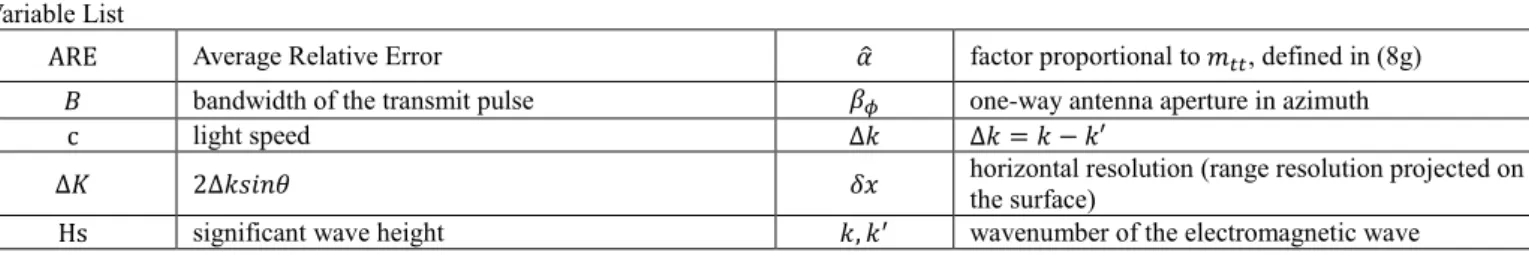
Table I

RADAR PARAMETERS IN THE SIMULATIONS

Radar frequency 13.5 GHz

Central incidence 13°

3 dB Beam width in azimuth, 𝛽𝜙 8.6°

Radar range resolution 1.5 m

Integration time 33 ms

Platform velocity 100 m/s

Flight height 2000 m

In section III.A, we first discuss the dependence of 𝑃𝑠𝑝 (K, Φ)

with azimuth and the role of the different terms contributing to this dependence. In section III.B, we analyze the trend of the azimuthally-averaged speckle energy with wave number and more particularly the impact of sea-state conditions on this trend.

In the results presented below, 𝑚𝑡𝑡 was calculated with (8i)

and for various empirical ocean wave spectra 𝐹(𝐾, Φ). For a pure wind wave situation, 𝐹(𝐾, Φ) was chosen as the Elfouhaily spectrum - named EL [17] hereafter. A swell component was added in some simulations, with the swell spectrum expressed as a Gaussian function as in [18].

Overall, three categories of cases of sea surface conditions were considered in our simulations. The parameters of the sea conditions for different categories are listed in Table II, including the wind speed U10, the wave inverse age Ω, the peak

wave length λ𝑝, the significant wave height Hs.

Table II

SEA SURFACE CONDITIONS USED FOR THE SIMULATION Case 1

Pure wind wave

Case 2 Mixed sea Case 3 Mixed sea Wind wave component 𝑈Ω = 0.84 10= 10 𝑚/𝑠, 𝑈Ω = 0.84 10= 10𝑚/𝑠, 𝑈Ω = 0.84 10= 10 𝑚/𝑠, Swell component Hs= 2m, λ𝑝= 400 m, propagating along the wind direction

Hs=4m, λ𝑝= 200

m, propagating along the wind direction

𝜔𝑑 in (8i) is the wave scale limit which makes the

quasi-specular scattering approximation valid. We determined 𝜔𝑑 by

the following method. At near-nadir incidence angles, the Physical Optics model, hereafter referred to as PO model, is considered accurate enough as long as polarization effects remain negligible, that is in the first 20 to 25° incidence away from nadir [14], [19], [20]. Here PO is referred as the reference model. Firstly, we calculate the backscattering coefficients by PO and EL spectrum for the sea surface conditions. On the other hand, the backscattering coefficients by the approximation model-Quasi-specular scattering model [14] is expressed as: 𝜎𝑄𝑆0 (𝜃) =|𝑅𝑒| 2 𝑚𝑠𝑠𝑒𝑠𝑒𝑐 4_{( 𝜃) 𝑒𝑥𝑝( −}𝑡𝑎𝑛2(𝜃) 𝑚𝑠𝑠𝑒 ) (9) 𝑚𝑠𝑠𝑒= ∫ 𝐾₀𝐾𝑑 2𝐹(𝐾)𝑑𝐾 (10)

Secondly, fitting (10) to 𝜎0_{(θ) values generated with the PO}

model in the incidence range of 0 to 18°, 𝑅𝑒 and 𝑚𝑠𝑠𝑒 can be

inversed. Thirdly, we obtain 𝐾𝑑 according to (10) from the

inversed 𝑚𝑠𝑠𝑒. Finally, 𝜔𝑑 is calculated by 𝜔𝑑2= 𝐾𝑑𝑔 for the

case of deep water.

In order to estimate 𝑁𝑖𝑛𝑡 , we calculate the modulation

spectrum 𝑃𝑚𝑜𝑑(𝐾, Φ) due to the tilting waves as in[11]:

𝑃𝑚𝑜𝑑(𝐾, Φ) =√2𝜋_𝐿 𝜙 (𝑐𝑡𝑔𝜃 − 𝜕𝑙𝑛𝜎0 𝜕𝜃 ) 2 𝐾2_{𝐹(𝐾, Φ) (11)} where 𝜎0 _{is obtained by (9).}

A. Variations with the look angle and impact of sea state conditions

From (8a) the energy of the speckle noise spectrum is determined by 𝑁𝑡𝑜𝑡(𝛷) for a given radar configuration. From

(8b), 𝑁𝑡𝑜𝑡(𝛷) is a function of 𝑁𝑠𝑢𝑟𝑓, 𝑁𝑝𝑙𝑎𝑡𝑓, and 𝑁𝑖𝑛𝑡, where

𝑁𝑠𝑢𝑟𝑓 is independent of the azimuth look direction, while

𝑁𝑝𝑙𝑎𝑡𝑓, and 𝑁𝑖𝑛𝑡 change with it.

In this section we discuss the variations of 𝑁𝑠𝑢𝑟𝑓 with the

sea surface conditions, and those of 𝑁𝑝𝑙𝑎𝑡𝑓 and 𝑁𝑖𝑛𝑡 with the

azimuth look direction (as for an azimuthally scanning radar). For convenience, the relative look direction Φ is defined as Φ = Φ1− Φ𝑝𝑙𝑎𝑡𝑓, where Φ1 is azimuth angle with respect to

geographical North and the latter is the flight direction. We first illustrate in Fig. 1 the variation of 𝑁𝑠𝑢𝑟𝑓 with wind

speed 𝑈10 for three different values of the inverse wave age

( Ω = 0.84 , 1 and 2), corresponding to the fully developed, mature and young sea. As can be seen in Fig. 1, 𝑁𝑠𝑢𝑟𝑓

significantly increases with wind speed for all wave ages. For example, for fully-developed situations 𝑁𝑠𝑢𝑟𝑓 increases from

about 4 to about 13 over the wind speed range 6 to 18 m/s. As shows the trend with wind speed, the sensitivity of 𝑁𝑠𝑢𝑟𝑓 to

wind speed is much higher for fully-developed conditions than for young waves. From (8i), this is due to the variation of the velocity variance 𝑚𝑡𝑡 with both wind and wave age.

Fig. 1. 𝑁𝑠𝑢𝑟𝑓 variation with wind speed under different inverse wave ages

(green, blue, red, for respectively 0.84, 1, 2)

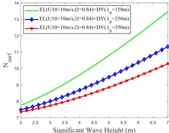
To illustrate the effect of swell on 𝑁𝑠𝑢𝑟𝑓, Fig. 2 shows the

variations of 𝑁𝑠𝑢𝑟𝑓 with the significant height Hs of the swell

component with the swell peak wavelength λ𝑝=

150 𝑚, 250𝑚, 350 𝑚 . It shows that 𝑁𝑠𝑢𝑟𝑓 increases with the

swell Hs when keeping the wind wave component constant. When the swell Hs increases from 2 m to 7 m, 𝑁𝑠𝑢𝑟𝑓 is

multiplied by 1.7, 1.5, 1.4 for the swell peak wavelength λ𝑝=

150 𝑚, 250 𝑚, 350 𝑚, respectively.

Fig. 2. 𝑁𝑠𝑢𝑟𝑓 variation with wind speed for a mixed sea condition with fully

developed wind waves and swell of different wavelengths (green, blue, red for 150, 250 and 350 m, respectively)

From Fig. 1 and 2, we draw a conclusion that 𝑁𝑠𝑢𝑟𝑓 increases

with wind speed and significant height Hs. The sensitivity with wind speed is much more important than with the significant height of a swell component. It is because that from (8e) 𝑁𝑠𝑢𝑟𝑓

is determined by the sea surface condition through the velocity variance 𝑚𝑡𝑡 , which is dominated by the wind waves because

of their higher surface velocities; the addition of a ‘gentle’ swell does not increase 𝑚𝑡𝑡 (𝑁𝑠𝑢𝑟𝑓) significantly.

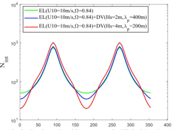
The parameter 𝑁𝑖𝑛𝑡 in (8f) is dependent on the sea conditions

and on the radar azimuth looking angle with respect to the flight direction (8g to 8h). Fig. 3 shows the variations of 𝑁𝑖𝑛𝑡 with

the relative look direction Φ , when the wind wave direction coincides with the flight direction, for a sea-state with a 10 m/s fully developed wind wave situation (case 1) and for two cases of mixed sea with swell added to the wind sea (swell Hs=2m and 4m for cases 2 and 3 respectively). The swell direction was set aligned with the wind wave direction in cases 2 and 3.

It shows that for each case, 𝑁𝑖𝑛𝑡 reaches maximum values in

the cross-wave/cross-track direction, while it gets minimum values along the wave propagation direction which coincides in this case with the flight direction. This is because 𝑁𝑖𝑛𝑡 is

proportional to 𝑃𝑚𝑜𝑑∗ / 𝑚𝑡𝑡 according to (8f), where 𝑃𝑚𝑜𝑑∗ is the

sum of the modulation spectrum 𝑃𝑚𝑜𝑑, which is related to the

This latter is much smaller than 𝑃𝑚𝑜𝑑 . Thus, 𝑁𝑖𝑛𝑡 is mainly

dominated by the ratio 𝑃𝑚𝑜𝑑/ 𝑚𝑡𝑡 . 𝑃𝑚𝑜𝑑 is maximum

(minimum) along (cross) the wave propagation direction, thus 𝑁𝑖𝑛𝑡 is minimum (maximum) in this direction since 𝑚𝑡𝑡

does not change with the azimuth anlge. Fig. 3 also shows that the sea-state condition impacts 𝑁𝑖𝑛𝑡 mainly in the along-wave

direction with the smallest values observed for the highest significant wave height ( 𝑁𝑖𝑛𝑡 = 40, 30, 10 for the sea

conditions of case1, case 2 and case 3, respectively). In the cross-wave direction, the order of magnitude of 𝑁𝑖𝑛𝑡 is about

30 to 100 times higher than in the along wind direction.

Fig. 3. 𝑁_𝑖𝑛𝑡 as a function of the azimuth look direction (with respect to the flight direction) when the flight direction is aligned with wind-wave direction. The green, blue, and red curves are for sea surface conditions of cases 1 to 3, respectively (see text)

From (8d) and (6) one notes that 𝑁𝑝𝑙𝑎𝑡𝑓 is dependent only

on the radar looking direction in azimuth with respect to the advection direction, whereas 𝑁𝑡𝑜𝑡 varies with all parameters

(flight direction, sea surface conditions and radar azimuth angle). Fig. 4 shows 𝑁𝑝𝑙𝑎𝑡𝑓 and 𝑁𝑡𝑜𝑡 variations with the

relative azimuth looking direction for the pure wind wave case (case 1, EL spectrum with 𝑈10= 10 𝑚/𝑠, Ω = 0.84) when

the flight track is perpendicular to the wind and wave directions. It shows that 𝑁𝑝𝑙𝑎𝑡𝑓 is zero along the flight direction and

reaches maximum values in the across flight direction. It is obvious from (6) since 𝑁𝑝𝑙𝑎𝑡𝑓 is determined by sinΦ, where Φ

is the azimuth angle relative to the radar flight direction. Fig. 4 also shows that along the flight direction (at 0° and 180°), 𝑁𝑡𝑜𝑡

is minimum, however, not equal to zero; it is because in this direction 𝑁𝑡𝑜𝑡 is mainly determined by 𝑁𝑠𝑢𝑟𝑓 along the flight

direction (in this direction 𝑁𝑝𝑙𝑎𝑡𝑓 is zero), and 𝑁𝑖𝑛𝑡 is big

enough to avoid a null value of 𝑁𝑡𝑜𝑡. In contrast, in the across

flight direction, just along the wind or wave direction, 𝑁𝑖𝑛𝑡 is

minimum, and 𝑁𝑡𝑜𝑡 is determined by both 𝑁𝑝𝑙𝑎𝑡𝑓 and 𝑁𝑖𝑛𝑡.

Hence, in these conditions, the number of independent samples 𝑁𝑡𝑜𝑡 is sufficient to avoid large value of the speckle

noise spectrum when the antenna looks in the along-track direction.

Fig. 4. Variation of 𝑁𝑝𝑙𝑎𝑡𝑓 (in red) and 𝑁𝑡𝑜𝑡 (in blue) with the azimuth look

direction (with respect to the flight direction) when the flight direction is perpendicular to the wind-wave direction. The sea surface conditions are those of case 1 (see text).

Now we study the effect of the angle between the flight direction and the wind (or wave) direction on the number of the independent samples 𝑁𝑡𝑜𝑡 (Φ). Fig. 5 shows 𝑁𝑡𝑜𝑡(Φ), for the

same conditions as in Fig. 4 (fully developed wind waves), when the angle between the flight track and the wave direction is 0°, 30°, 60° and 90°. It shows that 𝑁𝑡𝑜𝑡 always reaches a

maximum when the radar looks nearly perpendicularly to the flight direction, and is minimum when it looks along the flight direction. The minimum values of 𝑁𝑡𝑜𝑡 is almost constant for

different relative angles between the flight track and the wave direction. It is because along the flight direction, 𝑁𝑡𝑜𝑡 is

dominated by 𝑁𝑠𝑢𝑟𝑓 , which is independent of azimuth. In

opposite, the maximum values of 𝑁𝑡𝑜𝑡 decrease with relative

angle between the flight track and the wave direction. For the developed wind wave with 𝑈10 =10m/s, the maximal 𝑁𝑡𝑜𝑡

decreases from 44 to 22 when this angle changes from 0° to 90°. When the wave direction coincides with the flight direction, both 𝑁𝑚𝑜𝑣 and 𝑁𝑖𝑛𝑡 reach their maximum values in the same

direction. When the relative angle between the flight track and the wave direction increases, the angle between the direction where 𝑁𝑚𝑜𝑣 is maximum and 𝑁𝑖𝑛𝑡 is maximum also increases,

which results in a lower value of the maximum value of 𝑁𝑡𝑜𝑡

and a more stable value of 𝑁𝑡𝑜𝑡 with look angle outside a sector

of ±30° along-track.

In summary, the behavior of the total number of independent samples, 𝑁𝑡𝑜𝑡, has a multi-harmonic shape with minimum of

𝑁𝑡𝑜𝑡 always in the along-track direction and a minimum value

which depends on sea-state. The azimuth position of the maximum of 𝑁𝑡𝑜𝑡 varies with angle between the flight direction

and wave propagation direction, and its level is also dependent of both sea-state and relative direction between waves and flight.

In order to study the role of 𝑁𝑖𝑛𝑡 in this general behavior of

𝑁𝑡𝑜𝑡, we define the ratio 𝑅𝑖𝑛𝑡 of the contribution of 𝑁𝑖𝑛𝑡 to the

total speckle noise spectrum 𝑃𝑠𝑝:

𝑅𝑖𝑛𝑡= 1 𝑁𝑖𝑛𝑡 1 𝑁𝑖𝑛𝑡 + 1 𝑁𝑝𝑙𝑎𝑡𝑓 = 𝑁𝑝𝑙𝑎𝑡𝑓 𝑁_𝑖𝑛𝑡+𝑁_{𝑝𝑙𝑎𝑡𝑓} (12)

This ratio indicates the impact of non-neglecting the variation of the main factor in the four-frequency moment near the origin in the development of speckle noise spectrum while considering a moving surface.

Fig. 5. 𝑁𝑡𝑜𝑡 as a function of the azimuth look direction (with respect to

the flight direction) for different flight angles with respect to the wave direction: green, blue, red, yellow for 0°, 30°, 60°,90°, respectively. The sea surface conditions are those of case 1 (fully developed wind

Fig. 6. 𝑅𝑖𝑛𝑡 as a function of the relative look direction withthe color code and sea surface conditions similar to Fig. 5.

For the same sea conditions as in Fig. 5, Fig. 6 shows 𝑅𝑖𝑛𝑡 as

a function of the radar azimuth look angle (with respect to the flight direction) for different wave propagation directions. It shows that 𝑅𝑖𝑛𝑡 ranges between almost 0% and 60% depending

on the azimuthal look angle. It is minimum in the cross-wave direction for any flight directions. It is because from (8f) and (8h), when observing in the direction perpendicular to the wave propagation P𝑚𝑜𝑑 approaches zero, which leads to large 𝑁𝑖𝑛𝑡

values. Fig. 6 shows that the maximum values of 𝑅𝑖𝑛𝑡 change

from 38% to 58% when the flight direction goes from 0° to 90° with respect to the wave propagation direction. When this angle is 90° (cyan curve in Fig. 6), R𝑖𝑛𝑡 is maximum in the along

wave propagation direction. It is because, for an angle of 90°

between the flight direction and the waves, 𝑃𝑚𝑜𝑑 (or

(𝑁𝑖𝑛𝑡)−1 ) approaches to its maximum, whilst (𝑁𝑝𝑙𝑎𝑡𝑓)−1 is

minimum. For angles different from 90°, there is no direction where (𝑁𝑖𝑛𝑡)−1 and (𝑁𝑝𝑙𝑎𝑡𝑓)−1 are simultaneously maximum

and minimum, respectively, so that 𝑅𝑖𝑛𝑡 peak values cannot get

the same maximum as for the case of angle of 90° .When changing from 90° to 0° the locations of the maximum of the curves are shifted to the cross-wave direction. For flight directions of 0 and 30° with respect to the wave direction, the variation with the direction is more complex with secondary maxima appearing. A maximum value of almost 60% 𝑅𝑖𝑛𝑡 as

found in these fully developed conditions indicate that the term 𝑁𝑖𝑛𝑡 as taken into account in our model is not negligible for

certain conditions of observations.

B. Omni-directional speckle noise spectrum

In this section, we analyze the omni-directional spectrum of speckle noise as a function of the surface wavenumber 𝐾, and its dependence with wind speed, sea-state and radar configurations.

The omni-directional speckle noise spectrum is defined as:

𝑃𝑠𝑝(𝐾) = ∫ 𝑃₀2𝜋 𝑠𝑝(𝐾, Φ)𝑑Φ (13)

Besides the density of the speckle noise spectrum, we also focus on a Signal-To-Noise ratio (SNR), which is defined as the ratio of the signal spectrum 𝑃1(𝐾, Φ) in (A17) and the noise

spectrum 𝑃𝑠𝑝(𝐾, Φ) in (8a),

SNR(𝐾, Φ)=2𝜋𝐾𝑝𝑁𝑡𝑜𝑡(Φ)𝑡𝑟𝑖 (_2𝜋𝐾𝐾

𝑝) 𝑃𝑚𝑜𝑑(𝐾, Φ) (14)

Accordingly, an azimuthally-integrated SNR value is defined as:

SNR(𝐾) =_2𝜋1 ∫ 𝑆𝑁𝑅(𝐾, Φ)₀2𝜋 𝑑Φ (15)

Firstly, we study the effect of wind speed on 𝑃𝑠𝑝(𝐾), based

on our model with the EL wave spectrum used as input with a prescribed wind speed 𝑈10and wave age Ω.

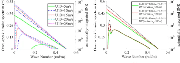
Fig. 7. Omni-directional speckle noise spectrum (left Y-axis) and SNR (right Y-axis) as a function of the wavenumber K for different wind speeds 𝑈10 = 5,10,18 m/s and for fully developed wind waves

Fig. 8. Omni-directional speckle noise spectrum (left Y-axis) and SNR (right Y-axis) as a function of the wavenumber K for the mixed sea, with

the different Hs for the swell component

Fig. 7 shows 𝑃𝑠𝑝(𝐾) (left Y-axis) and SNR (𝐾) (right Y-axis)

for different wind speed values (taken at the height of 10 m), namely every 5 m/s from 5 to 25m/s and with an inverse wave age of 0.84 (fully-developed waves). It shows that the energy of the speckle spectrum is not very sensitive to the wind speed. The relationship between the speckle energy and the wind speed is not strictly monotonous: the energy for 5 m/s is a little lower than that for 10 m/s, but is a little larger than that for 15m/s. As the wind speed continues to increase from 15 to 25 m/s, both the value at the origin (𝐾 =0) and the slope of the trend with 𝐾 decreases. The change of 𝑃𝑠𝑝(𝐾) with wind speed

is due to the azimuthally averaged 𝑁𝑡𝑜𝑡 factor, which is

dependent of wind speed through the terms in 𝑁𝑠𝑢𝑟𝑓 and 𝑁𝑖𝑛𝑡.

As described in section III.A, 𝑁𝑠𝑢𝑟𝑓 is determined by the

velocity variance of the sea surface 𝑚𝑡𝑡 , while 𝑁𝑖𝑛𝑡 is

dominated by the ratio of the modulation spectrum 𝑃𝑚𝑜𝑑 in (11)

and 𝑚𝑡𝑡 . With wind speed increasing, on one hand 𝑚𝑡𝑡 and

𝑁𝑠𝑢𝑟𝑓 increase, but on the other hand 𝑁𝑖𝑛𝑡 decreases because

𝑃𝑚𝑜𝑑 increases more than 𝑚𝑡𝑡 does. The combination of these

effects (enlarging 𝑁𝑠𝑢𝑟𝑓 but reducing 𝑁𝑖𝑛𝑡 ) lead to a not

monotonous dependence of speckle energy with wind speed. Fig. 7 also shows that SNR increases greatly with the wind speed, the SNR maximum appear at the peak wave number.

We also studied the effect of the developing stage of the wind waves. Our results indicate (not shown here) that 𝑃𝑠𝑝(𝐾)

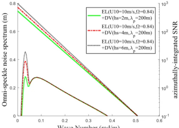
decreases slightly with the inverse wave age for the same wind. The impact of an additional swell is illustrated in Fig. 8, which shows 𝑃𝑠𝑝(𝐾) for a mixed sea, with the wind wave

component for 𝑈10= 10 𝑚/𝑠, inverse wave age Ω = 0.84 and

a swell component with a peak wavelength λ𝑝= 200 𝑚 and a

significant height 𝐻𝑠 = 2 m, 4 m, and 6 m . It shows that the energy of the noise spectrum is not very sensitive to the swell

wave height, when all other parameters are kept constant, 𝑃𝑠𝑝(𝐾) increases slowly but monotonously when Hs of the

swell component increases from 2 m to 6 m. It is because, as described in section III.A, 𝑚𝑡𝑡 (𝑁𝑠𝑢𝑟𝑓 ) is dominated by the

wind waves because of their higher frequencies, while the addition of the swell does not increase 𝑚𝑡𝑡 (𝑁𝑠𝑢𝑟𝑓) significantly.

On the other hand, from (8f), since 𝑚𝑡𝑡 does not change a lot

𝑁𝑖𝑛𝑡 is dominated by the modulation spectrum 𝑃𝑚𝑜𝑑 , which is

sensitive to the long waves. Thus, the addition of swell increases 𝑃𝑚𝑜𝑑 , and accordingly decreases 𝑁𝑖𝑛𝑡 . The

combination of the two effects (enlarging 𝑁𝑠𝑢𝑟𝑓 a little but

reducing 𝑁𝑖𝑛𝑡), leads to a monotonous increase of the energy of

the noise spectrum with Hs of the swell.

We also studied the effect of different peak wavelengths of the swell component. Our results indicate (not shown here) that 𝑃𝑠𝑝(𝐾) increases very slightly with the swell λ𝑝 when the other

parameters are kept constant. Thus, for swell the speckle is almost not affected by its dominant wavelength (or period).

In summary, for the radar configuration chosen here the azimuthally-integrated value of the speckle noise spectrum is not very sensitive to the sea surface conditions because the effects of the sea conditions on the density of speckle noise spectrum by 𝑁𝑠𝑢𝑟𝑓 and 𝑁𝑖𝑛𝑡 are opposite and comparable.

We will see in section VI, that the conclusion may change when considering other radar frequencies, central incidences, 3dB beam width in azimuth, platform speed and platform height.

IV. EXPERIMENTAL ESTIMATE OF THE SPECKLE NOISE SPECTRUM

Two empirical methods have been proposed and implemented in the past for estimating the speckle noise spectrum from the backscattered intensity observations themselves: the “post-integration” method [3] and the cross-spectrum method first applied on SAR data [2] and then adapted to the real-aperture scanning configuration [10]. The two methods require that the radar samples correspond to overlapping sea surface areas for adjacent integration times. With the observation configuration of the airborne KuROS radar [10] both methods, either based on a cross-spectrum analysis or on different post-integrated signal are possible. Here, we choose the method based on different post-integrated signals because it optimizes the overlapping areas of the different signal samples used to estimate the speckle noise spectrum.

We recall first that KuROS is a Ku-band (f=13.5GHz) radar, with a near-nadir pointing rotating antenna, which provides the backscattering coefficients in the incidence range from about 5° to 18° and the azimuth range of 0 to 360° . The data sets analyzed here come from KuROS flights carried out in the northwestern part of the Mediterranean Sea as part of the Hymex experiment [10], [12].

A speckle spectrum estimation 𝑃𝑠𝑝(𝐾, Φ) can be derived

from the measured radar cross-section 𝜎0 _{fluctuation spectra.}

Let δ𝜎0_{(x, Φ) be the fluctuation function of the measured 𝜎}0

along the horizontal axis x (taken as aligned with the incidence plane) in the azimuth direction, and 𝑃𝜎0(𝐾, Φ) its spectral

density as a function of the wave number modulus in the azimuth direction. Then, as shown in (A39) 𝑃𝜎0(𝐾, Φ) is given

by:

𝑃𝜎0(𝐾, Φ) ≅ 𝑃_𝐼𝑅(𝐾, Φ)𝑃_𝑚𝑜𝑑(𝐾, Φ) + 𝑃_𝑠𝑝(𝐾, Φ)

(16) In (16), 𝑃𝜎0(𝐾, Φ) is obtained in each direction Φ from the

radar data, as the power spectrum of the relative fluctuations along the x axis (look direction) of 𝜎0_{. In order to obtain the}

speckle noise spectrum 𝑃𝑠𝑝(𝐾, Φ) , from this expression, we

used the post-integration method proposed in [3]. This method makes use of 𝜎0 _{values estimated – for the same raw data- over}

two different integration durations (𝑇𝑖𝑛𝑡 and 𝑁 ∙ 𝑇𝑖𝑛𝑡 ) and

assumes that the speckle reduction between the two cases (𝑇𝑖𝑛𝑡

and 𝑁 ∙ 𝑇𝑖𝑛𝑡) is of a factor N. Combining the spectrum of signal

fluctuation calculated over the period of 𝑁 ∙ 𝑇𝑖𝑛𝑡, (𝑃𝜎0)𝑁𝑇𝑖𝑛𝑡 ,

and the one resulting from the average of 𝑁 spectra each calculated over the period of 𝑇𝑖𝑛𝑡, 〈(𝑃𝜎0)_{𝑇𝑖𝑛𝑡}〉_𝑁,and assuming

that the wave contribution 𝑃𝑚𝑜𝑑 is identical in the two cases,

𝑃𝑠𝑝(𝐾, Φ) can be obtained:

𝑃𝑠𝑝(𝐾, Φ) =_𝑁−1𝑁 (〈(𝑃𝜎0(𝐾, Φ))𝑇𝑖𝑛𝑡〉𝑁− (𝑃𝜎0(𝐾, Φ))𝑁𝑇𝑖𝑛𝑡)

(17) Here for KuROS, we used 𝑇𝑖𝑛𝑡=33ms and N=3.

We recall here that KuROS range resolution is 1.5 m, leading to a horizontal resolution at the central incidence (13.5°) of ≈ 6.5 m. In the analysis presented here below, the spectral analysis is carried out by considering the horizontal footprint covered by the 8° to 18° incidence range, i.e., at ±5° from the central incidence angle 13°. This corresponds to a footprint of 475m or 710 m for the standard flight levels of 2000 m and 3000m, respectively.

The energy density spectra are binned in 64 wavenumbers and 60 azimuth directions. By fitting each azimuthal estimate of 𝑃𝑠𝑝_𝑚𝑒𝑎𝑠(𝐾, Φ) to the functional shape (8a), we obtain an

empirical estimate of the total number of independent samples 𝑁𝑡𝑜𝑡_𝑚𝑒𝑎𝑠 (Φ ) and of 𝐾𝑝 (Φ ). By averaging 𝐾𝑝 (Φ ) over the

azimuth angles (0 to 360°), we obtain a mean 𝐾𝑝, and hence an

estimate of the horizontal effective resolution 𝛿𝑥 = (𝐾𝑝)−1.

The results on 𝑁𝑡𝑜𝑡_𝑚𝑒𝑎𝑠 (Φ ) and their omni-directional

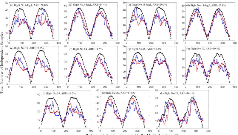
counterpart (estimated from (13)) are shown in Fig. 10 and 9, respectively for 9 different situations. They are discussed together with the model results in the next section.

V. VALIDATION OF THE MODEL OF SPECKLE NOISE SPECTRUM

In this section, we use the estimates of speckle noise spectrum from KuROS to validate the model presented in section III. In total, there are 12 KuROS flights with coincident wind and wave measurements from the ‘Lion’ buoy (see [10]). From this data set, we have rejected in our analysis 3 cases (flights 9, 16 and 22) because it turned out that for these flights 𝜎0 _{values are more than 5dB below normal, which leads in an}

abnormal speckle noise spectrum. For flight 4 and 11, the plane flew twice over the buoy with different flight directions. Table III lists for the 11 cases analyzed hereafter, the wind and wave parameters measured from the ‘Lion’ Buoy, namely the wind speed at 10 m height 𝑈10, wind direction φ𝑤𝑖𝑛𝑑, the significant

height Hs, the peak frequency 𝑓𝑝, wave direction φ𝑤𝑎𝑣𝑒. In the

same table, the inverse wave age Ω is listed to indicate the developing stage of the wind waves. Here Ω is calculated as Ω = 𝑈10√𝑘𝑝/𝑔, where 𝑘𝑝is the peak wavenumber is related to

𝑓𝑝 by the dispersion relationship in deep water 𝑘𝑝𝑔 = (2𝜋𝑓𝑝)2.

The omni-directional speckle noise spectrum 𝑃𝑠𝑝_𝑚𝑜𝑑(𝐾)

from the model was estimated using (8a) to (8i) with 𝐾𝑝 estimated from the empirical 𝛿𝑥 value; the wind and wave

parameters shown in Table I were used to estimate the velocity variance 𝑚𝑡𝑡 which affects the 𝑁𝑖𝑛𝑡 and 𝑁𝑠𝑢𝑟𝑓 terms according

to (8e) and (8f). For that, a wind wave spectrum following the Elfouhaily’s expression was calculated for the observed wind speed and wave age at the buoy location. The modulation spectrum 𝑃𝑚𝑜𝑑 which affects the 𝑁𝑖𝑛𝑡 term (8f) was taken as

provided by the Kuros data processing. 𝑘𝑑 in (8i) was

We also calculated 𝑃′𝑠𝑝_𝐽𝑎𝑐(𝐾) and 𝑁′𝐽𝑎𝑐(Φ) by using (6)

which come from Jackson’s model [11], and using the same input parameters 𝐾𝑝 and 𝑃𝑚𝑜𝑑 described just above. μ was

estimated by using (7).

Finally we compared 𝑃𝑠𝑝(𝐾) and 𝑁𝑡𝑜𝑡(Φ) predictions from

our model, 𝑃′𝑠𝑝_𝐽𝑎𝑐(𝐾) and 𝑁′𝐽𝑎𝑐(Φ) predictions from

Jackson ’s model in [11], and 𝑃𝑠𝑝_𝑚𝑒𝑎𝑠(𝐾) and 𝑁𝑡𝑜𝑡_𝑚𝑒𝑎𝑠 (Φ )

estimated from the KuROS data. In order to estimate the error between the measurements and model values, an Average Relative Error is defined as:

ARE =_𝑁1∑ |𝑉𝑖_𝑚𝑒𝑎𝑠−𝑉𝑖_𝑚𝑜𝑑𝑙

𝑉_{𝑖_𝑚𝑜𝑑𝑙} | 𝑁

𝑖=1 (18)

Where 𝑉𝑖𝑚𝑒𝑎𝑠 are the measurements of 𝑃𝑠𝑝(𝐾) (or 𝑁𝑡𝑜𝑡(Φ)) at

𝐾𝑖 (or Φ𝑖) , 𝐾𝑖= 𝑖∆𝐾 , Φ𝑖= 𝑖∆Φ, ∆𝐾 =₆₄1 𝐾𝑚𝑎𝑥, 𝐾𝑚𝑎𝑥=_𝛿𝑥𝜋,

𝛿𝑥 ≈ 6.5 m, ∆Φ = 6°, 𝑉𝑖_{𝑚𝑜𝑑𝑙} are the calculation results from

the model presented in section II. Considering the theoretical horizontal resolution 𝛿𝑥 is about 6.5 m, KuROS can only detect the waves with the wavelength larger than at least 2 times the horizontal resolution. Thus, the detectable maximum 𝐾detc _𝑚𝑎𝑥≈ 0.24. On the other hand, with the limit of 𝐾𝐿𝑦≫

1 [1],𝐿𝑦= 𝐿_𝑦∗ 2√2𝑙𝑛2, 𝐿𝑦 ∗ _{= 2 ∗ 𝐻 ∗ 𝑡𝑎𝑛 (}𝛽𝜙 2) ∗ 𝑐𝑜𝑠 −1_{𝜃 , where H}

is the flight height, 𝛽ϕ= 8.6° , the minimal detectable

𝐾𝑑𝑒𝑡𝑐_𝑚𝑖𝑛 is set as 0.038 rad/m. Therefore, 𝐾𝑖 is between

𝐾𝑑𝑒𝑡𝑐_𝑚𝑖𝑛 and 𝐾𝑑𝑒𝑡𝑐 _𝑚𝑎𝑥.

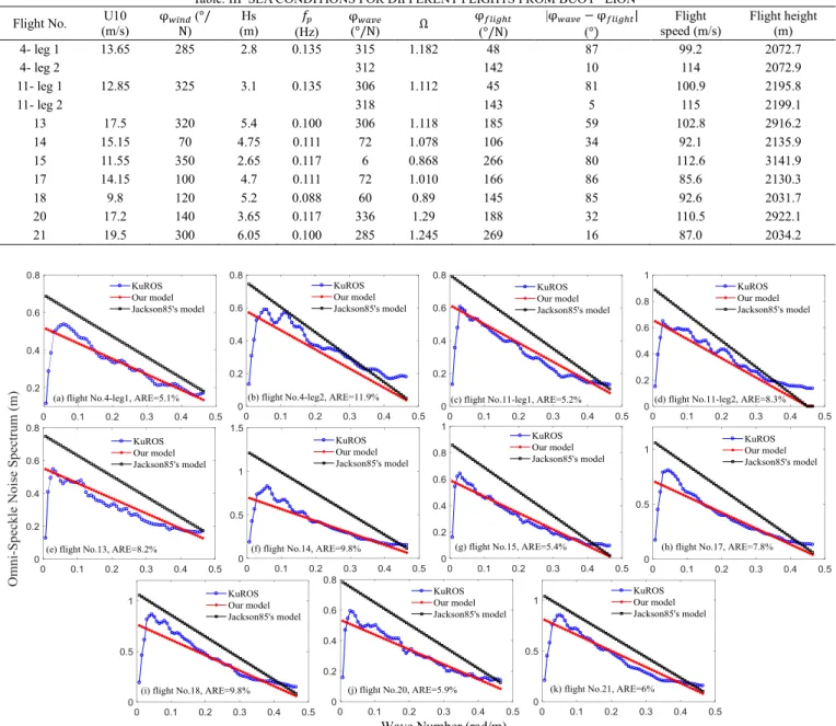
Table. III SEA CONDITIONS FOR DIFFERENT FLIGHTS FROM BUOY “LION” Flight No. _(m/s) U10 φ𝑤𝑖𝑛𝑑 (°/

N) Hs (m) 𝑓_𝑝 (Hz) φ𝑤𝑎𝑣𝑒 (°/N) Ω φ𝑓𝑙𝑖𝑔ℎ𝑡 (°/N) |φ𝑤𝑎𝑣𝑒− φ𝑓𝑙𝑖𝑔ℎ𝑡| (°) Flight speed (m/s) Flight height (m) 4- leg 1 13.65 285 2.8 0.135 315 1.182 48 87 99.2 2072.7 4- leg 2 312 142 10 114 2072.9 11- leg 1 12.85 325 3.1 0.135 306 1.112 45 81 100.9 2195.8 11- leg 2 318 143 5 115 2199.1 13 17.5 320 5.4 0.100 306 1.118 185 59 102.8 2916.2 14 15.15 70 4.75 0.111 72 1.078 106 34 92.1 2135.9 15 11.55 350 2.65 0.117 6 0.868 266 80 112.6 3141.9 17 14.15 100 4.7 0.111 72 1.010 166 86 85.6 2130.3 18 9.8 120 5.2 0.088 60 0.89 145 85 92.6 2031.7 20 17.2 140 3.65 0.117 336 1.29 188 32 110.5 2922.1 21 19.5 300 6.05 0.100 285 1.245 269 16 87.0 2034.2

Fig. 9. Omni-directional speckle noise spectrum as a function of wavenumber for the cases listed in Table III: panels (a, b, c, d, e, f, g, h, i, j, k) refer respectively to flights 4-leg1, 4-leg2, 11- leg 1, 11-leg 2, 13, 14, 15, 17, 18, 20, 21.The blue, red and black curves are for respectively, the empirical estimates from KuROS data, from our model, and from Jackson’s model

Fig. 9 (a) shows the omni-directional speckle noise spectra for the flight 4-leg 1, when the flight direction was nearly perpendicular to the wave direction. It shows that our model (red line) agrees well with the empirical estimates of the omni-directional speckle noise spectrum (blue line), with the error ARE below 5%, while Jackson’s model (black line) overestimates the omni-directional speckle noise spectrum at all 𝐾 and overestimates the decreasing trend with 𝐾. Fig. 10 (a)

shows for the same cases, 𝑁𝑡𝑜𝑡 (Φ ) as a function of the

observation azimuth angle with respect to the flight direction. It shows that 𝑁𝑡𝑜𝑡 (Φ ) from our model, and from Jackson’s

model, both show the minimum values at about the flight direction, in agreement with the empirical estimates. This was expected because at the flight direction, the value of 𝑁𝑝𝑙𝑎𝑡𝑓

approaches 1. In this along-track direction, 𝑁𝑡𝑜𝑡 from our

model is in better agreement with the empirical estimates than the result from Jackson’s model, because it is determined by 𝑁𝑠𝑢𝑟𝑓 proposed in our model. In contrast, for Jackson’s model

the time-varying properties of the sea surface are ignored which induces an underestimate of 𝑁𝑡𝑜𝑡 in the along-track direction. It

proves that the 𝑁𝑠𝑢𝑟𝑓 term as added in our model is necessary

to guarantee consistency, especially for look angles aligned with the flight direction. In a wide sector around the across-flight direction, 𝑁𝑡𝑜𝑡 from the Jackson’s model is overestimated

with respect to the empirical estimation. This is due to the omitted contribution of 𝑁𝑖𝑛𝑡 in the Jackson’s model which

comes from neglecting the variation of the main factor in the four-frequency moment near the origin. It proves that the term (𝑁𝑖𝑛𝑡)−1 added in our model is also necessary to guarantee

consistency with observations. In contrast Fig. 10 (a) shows that 𝑁𝑡𝑜𝑡(Φ) calculated with our model better agrees with the

empirically estimated 𝑁𝑡𝑜𝑡 (Φ ) over all azimuth angles. The

small remaining differences between the measured 𝑁𝑡𝑜𝑡 and

that calculated with our model may come from the statistical fluctuations of the measured 𝑁𝑡𝑜𝑡 (here we estimated 𝑁𝑡𝑜𝑡 as

averaged values over 6° bins in azimuth) or small remaining uncertainties on the geometry (incidence angle, azimuth angle). The other panels in fig. 9 and fig. 10 show the omni-directional speckle noise spectrum and 𝑁𝑡𝑜𝑡 for flights 11, 13,

14, 15, 17, 18, 20, 21 respectively, from which the same conclusions as those discussed in details for flight 4 can be drawn. The errors between the measured omni-directional speckle noise spectrum and that estimated by our model are all below 10%. The minimum values of 𝑁𝑡𝑜𝑡 predicted by our

model is of about 8 to 10 (Fig. 10) and agree well with the experimental values. The maximum values of 𝑁𝑡𝑜𝑡 are within

range 25 to 50, depending of the flight conditions.

It is interesting to note the different shapes of the 𝑁𝑡𝑜𝑡 curves

for different flight directions with respect to the wave direction. When the flight direction is aligned with the wave propagation direction (Fig. 10(b, d, k)), both the KuROS estimates and our model indicate a well-marked peak in the cross-track directions. This is very similar to the shape of the green curve in Fig. 5, namely the 𝑁𝑡𝑜𝑡 curve simulated with our model with the

flight-wave angle set as zero. In these conditions, azimuth variations from Jackson’s model remains close to the observations and to our model.

On the other hand, for the files when the flight direction is nearly perpendicular to the wave direction (Fig. 10(a, c, g,h, i)), instead of a well-shaped peak, a large plateau or a multi-peak signature is observed in the 𝑁𝑡𝑜𝑡 curves around the cross-wave

direction. This is very similar to the shapes of the blue curve in Fig. 5, namely the 𝑁𝑡𝑜𝑡 curve simulated with our model with

the flight-wave angle set as 90° . In these cases, the discrepancies with respect to Jackson’s model are the largest.

Overall, the comparisons with the empirical estimates of the density spectrum show that our model, in opposite to Jackson’s model is able to reproduce the main trend of the speckle density spectrum variations with azimuth and with wave number in a large variety of conditions. This validates our model and indicates that it is essential to consider a moving surface in the speckle model and to avoid over simplification in the expression of the scattering matrix moments.

Fig. 10. Total number of independent samples 𝑁𝑡𝑜𝑡 as a function of relative look direction. Each subgraph corresponds to that of Fig.9, withthe color code similar to Fig. 9.

VI. INFLUENCE OF RADAR CONFIGURATION ON THE SPECKLE SPECTRUM

Now that the model of speckle is validated under its limit of application (near-nadir incidence) we propose to extend its use to other configurations of observations while staying in the near-nadir configuration. In this section, we study the impact of the radar configurations on omni-directional speckle noise

spectrum.

Firstly, we examine the impact of the platform advection speed. Then we analyze the impact of the footprint dimension in azimuth (either by changing the beam aperture or the flight height). Finally, we discuss the influence of radar frequency and of incidence angle.

When we increase the platform speed, the azimuthally-averaged 𝑁𝑚𝑜𝑣 term increases, which leads to the larger

contribution of 𝑁𝑖𝑛𝑡 and smaller contribution of 𝑁𝑠𝑢𝑟𝑓. Fig. 11

show the omni-directional speckle noise spectrum when the flight speed is 300 m/s and other parameters are the same as those in Fig. 7 and Fig. 8, respectively.

(a) (b)

Fig. 11. Omni-directional speckle noise spectrum (left Y-axis) and SNR (right Y-axis) as a function of the wavenumber K for the flight speed of 300 m/s, the sea surface conditions are the same as those of Fig. 7 and Fig. 8 for (a) and (b), respectively.

From Fig. 11, it is observed that in this configuration, the density of omni-directional speckle noise increases monotonously and significantly with wind speed or Hs of swell. It is because in such cases, 𝑁𝑖𝑛𝑡 dominates the density of the

spectrum. The increase of the wind speed and Hs lead to a larger increase of 𝑃𝑚𝑜𝑑 than of 𝑚𝑡𝑡 , and a decrease of 𝑁𝑖𝑛𝑡 , which

contribute to the increase of the density of the spectrum. Compared with Fig. 7 and Fig. 8, it is found that when increasing the platform speed, the energy density of the noise spectrum is smaller, which leads to a larger SNR, and the detectability of the shorter waves (SNR>1) is increased.

Results when changing the altitude of the platform from 2000m to 5000 m are shown in Fig. 12. Increasing the flight height means a larger value of 𝐿𝜙 in (11), and hence a decrease

in 𝑃𝑚𝑜𝑑. This leads to a larger contribution of 𝑁𝑠𝑢𝑟𝑓 and smaller

contribution of 𝑁𝑖𝑛𝑡 with respect to our simulations of Fig. 7

and 8, and explains why the sensitivity to with speed or wave height is different from the case of Fig. 7 to 8.

Compared with Fig. 7 and Fig. 8, it can be seen that the omni-directional energy of the noise spectrum is slightly smaller, in particular at small 𝐾 . This is because the higher flight level results in a larger value of 𝐿𝜙 and hence of 𝑁𝑖𝑛𝑡 in (8f). On the

other hand, 𝑃𝑚𝑜𝑑∗ decrease with 𝐿𝜙. The combination of both

effects finally results in a smaller SNR. Furthermore, the larger sensitivity to wind-sea wave height as compared to Fig. 7 is because, for a higher flight height while keeping all other parameters constant, 𝑁𝑠𝑢𝑟𝑓 may become dominant in the

speckle energy spectrum. Increasing the wind speed (and so the wind wave Hs) induces an increase in 𝑚𝑡𝑡 and 𝑁𝑠𝑢𝑟𝑓, which

explains the decreasing trend of the density of the spectrum for increasing wind speed (Fig. 12(a)). Furthermore, as 𝑚𝑡𝑡 is

mainly determined by the wind waves and not very sensitivity to long swell, the impact of increasing Hs remains small in the swell dominated case (Fig.12(b)).

(a) (b)

Fig. 12. Omni-directional speckle noise spectrum (left Y-axis) and SNR (right Y-axis) as a function of the wavenumber K for the flight height of 5000 m, the sea surface conditions are the same as those of Fig. 7 and Fig. 8 for (a) and (b), respectively.

Next, we study the impact of the beam aperture in azimuth. Fig. 13 show the omni-directional speckle noise spectrum when

the 3dB beam width in azimuth 𝛽𝜙 is 17.2°, namely two times

that given in Table I, other parameters are the same as those used for Fig.7 and Fig. 8, respectively. When 𝛽𝜙 increases,

𝑁𝑚𝑜𝑣 is larger according to (8c) and (5c), and 𝑁𝑖𝑛𝑡 is also larger

according to (8f). The results show that the omni-directional energy of the noise spectra decreases. On the contrary, compared with Fig. 7 and Fig. 8, the SNR is not modified when 𝛽𝜙 is increased. It is because SNR∝ 𝑁𝑡𝑜𝑡∗ 𝑃𝑚𝑜𝑑 , where

𝑁𝑡𝑜𝑡 ∝ 𝛽𝜙, 𝑃𝑚𝑜𝑑∝ (𝛽𝜙)−1 . Correlatively, in this case,

similarly to the cases of Fig. 7 and 8, the energy of the speckle noise spectrum does not vary significantly with the sea conditions. The results illustrated by Fig. 13 also show that in terms of SNR, it is not equivalent to increase the footprint dimension by flying higher or by increasing the beam aperture in azimuth. SNR is not affected by increasing the footprint, whereas increasing the flight height results in a decrease of the SNR.

(a) (b)

Fig. 13. Omni-directional speckle noise spectrum (left Y-axis) and SNR (right Y-axis) as a function of the wavenumber K for 3dB beam width in azimuth 𝛽𝜙= 17.2°, the sea surface conditions are the same as those of Fig. 7 and Fig. 8 for (a) and (b), respectively.

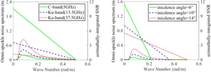
Now let us discuss the effect of the radar frequency. Fig. 14(a)

plots the omni-directional speckle noise spectrum in C-band (5GHz), Ku-band (13.5GHz) and Ka-band (37.5GHz) for case 1 of Table II (fully developed wind-waves with 𝑈10 = 10 m/s).

The other radar parameters are the same as those in Table I. From (5c), (8e) and (11), it is obvious that the radar frequency affects 𝑁𝑝𝑙𝑎𝑡𝑓 and 𝑁𝑠𝑢𝑟𝑓 through the electromagnetic wave

number 𝑘 and the 𝑚𝑡𝑡 value, and effects 𝑁𝑖𝑛𝑡 through 𝑘 , 𝑚𝑡𝑡

and the tilting sensitivity term 𝜕𝑙𝑛𝜎_𝜕𝜃0. With the radar frequency, 𝑘 and 𝑚𝑡𝑡 increase and 𝜕𝑙𝑛𝜎

0

𝜕𝜃 decreases, which leads to the

increases of 𝑁𝑖𝑛𝑡 , 𝑁𝑠𝑢𝑟𝑓 and 𝑁𝑝𝑙𝑎𝑡𝑓, then the decrease of

speckle spectrum decreases. On the other hand, the increase of the radar frequency also leads to the decrease of the modulation spectrum 𝑃𝑚𝑜𝑑 through 𝜕𝑙𝑛𝜎

0

𝜕𝜃 , see (11). The overall effect on

the speckle spectrum is that both the value at the origin (𝐾 =0) and the absolute value of the slope with 𝐾 decrease when increasing the electromagnetic frequency (C to Ka-band). The impact is important with a change by a factor of 2.9 on the value at the origin and on the linear slope. As for the SNR, Fig. 14(a)

shows that peak value increases by a factor of 4.2 from C-band to Ka-band and the detectability of the shorter waves (wavenumber for which SNR>1) significantly increases also. This shows that the overall impact of increasing the radar frequency is to increase the SNR, indicating that the lower values of 𝑃𝑚𝑜𝑑 when increasing the radar frequency (due to a

lower value of the tilt sensitivity term 𝜕𝑙𝑛𝜎_𝜕𝜃0) are over-balanced by the lower values of speckle energy. We can conclude from this, that for a same sea surface condition, same radar geometry and same radar bandwidth, a Ka-band configuration is better than a Ku or C-Band to minimize the speckle effect in the signal modulations.

Next, we study the effect of the radar incidence angle. Fig. 14(b) shows the omni-directional speckle noise spectrum at the