HAL Id: hal-00296452
https://hal.archives-ouvertes.fr/hal-00296452
Submitted on 22 Feb 2008
HAL is a multi-disciplinary open access
archive for the deposit and dissemination of
sci-entific research documents, whether they are
pub-lished or not. The documents may come from
teaching and research institutions in France or
abroad, or from public or private research centers.
L’archive ouverte pluridisciplinaire HAL, est
destinée au dépôt et à la diffusion de documents
scientifiques de niveau recherche, publiés ou non,
émanant des établissements d’enseignement et de
recherche français ou étrangers, des laboratoires
publics ou privés.
Eastern United States
P. N. Racherla, P. J. Adams
To cite this version:
P. N. Racherla, P. J. Adams. The response of surface ozone to climate change over the Eastern United
States. Atmospheric Chemistry and Physics, European Geosciences Union, 2008, 8 (4), pp.871-885.
�hal-00296452�
www.atmos-chem-phys.net/8/871/2008/
© Author(s) 2008. This work is distributed under the Creative Commons Attribution 3.0 License.
Chemistry
and Physics
The response of surface ozone to climate change over the Eastern
United States
P. N. Racherla1and P. J. Adams2
1Department of Engineering and Public Policy, Carnegie Mellon University, Pittsburgh, PA, USA
2Department of Civil and Environmental Engineering, and Engineering and Public Policy, Carnegie Mellon University,
Pittsburgh, PA, USA
Received: 18 June 2007 – Published in Atmos. Chem. Phys. Discuss.: 9 July 2007 Revised: 20 December 2007 – Accepted: 22 January 2008 – Published: 22 February 2008
Abstract. We investigate the response of surface ozone (O3)
to future climate change in the eastern United States by per-forming simulations corresponding to present (1990s) and future (2050s) climates using an integrated model of global climate, tropospheric gas-phase chemistry, and aerosols. A future climate has been imposed using ocean boundary con-ditions corresponding to the IPCC SRES A2 scenario for the 2050s decade. Present-day anthropogenic emissions and CO2/CH4mixing ratios have been used in both simulations
while climate-sensitive emissions were allowed to vary with the simulated climate. The severity and frequency of O3
episodes in the eastern U.S. increased due to future climate change, primarily as a result of increased O3 chemical
pro-duction. The 95th percentile O3mixing ratio increased by
5 ppbv and the largest frequency increase occured in the 80– 90 ppbv range; the US EPA’s current 8-h ozone primary stan-dard is 80 ppbv. The increased O3 chemical production is
due to increases in: 1) natural isoprene emissions; 2) hy-droperoxy radical concentrations resulting from increased water vapor concentrations; and, 3) NOxconcentrations
re-sulting from reduced PAN. The most substantial and statis-tically significant (p<0.05) increases in episode frequency occurred over the southeast and midatlantic U.S., largely as a result of 20% higher annual-average natural isoprene emis-sions. These results suggest a lengthening of the O3
sea-son over the eastern U.S. in a future climate to include late spring and early fall months. Increased chemical production and shorter average lifetime are two consistent features of the seasonal response of surface O3, with increased dry
deposi-tion loss rates contributing most to the reduced lifetime in all seasons except summer. Significant interannual variability is observed in the frequency of O3 episodes and we find that
it is necessary to utilize 5 years or more of simulation data
Correspondence to: P. N. Racherla ([email protected])
in order to separate the effects of interannual variability and climate change on O3episodes in the eastern United States.
1 Introduction
The reduction of surface ozone, which is harmful to hu-man, animal, and plant health, is an important objective of air quality policy for many governments. Surface ozone is produced through a complex set of photochemical reactions involving NOx(=NO+NO2) and volatile organic compounds
(VOCs). NOx and VOCs are emitted from anthropogenic
sources such as fossil fuel power plants, industrial activities and transportation, as well as natural sources such as light-ning and soil (NOx), and vegetation (biogenic VOCs such as
isoprene). The resulting ozone concentrations depend sen-sitively upon meterological parameters such as temperature, cloudiness, sunlight, wind speeds and the mixed layer depth. Therefore, changes in these meteorological parameters due to climate change will necessarily impact surface ozone con-centrations. However, the direction of change itself is often unclear because of multiple competing effects.
A major conclusion of many previous global modeling studies (Brasseur et al., 1998; Stevenson et al., 2000; Zeng and Pyle, 2003; Liao et al., 2006; Racherla and Adams, 2006), which have assessed the effect of future climate change on global tropospheric ozone is that the global av-erage burden of ozone decreases because of the increased destruction of ozone due to increased water vapor concen-trations. In these studies, although ozone chemical produc-tion increases it is dominated by the increased destrucproduc-tion of ozone on a global scale in the absence of changes in emissions. On the other hand, Collins et al. (2003); Zeng and Pyle (2003) suggest that the stratosphere-troposphere ex-change of ozone is likely to increase due to climate ex-change, which increases tropospheric ozone. Hauglustaine et al. (2005) predict an increase in the upper tropospheric ozone
concentrations due to climate change, which is primarily due to increased lightning NOxcaused by more intense
convec-tive activity.
While a number of previous modeling studies (Sillman and Samson, 1995; Aw and Kleeman, 2003; Baertsch-Ritter et al., 2004; Dawson et al., 2007) have focused on the effect of individual meteorological parameters on surface ozone, only a few studies have assessed holistically the effect of fu-ture climate change. One major conclusion of the former kind of modeling studies is that ozone increases with tem-perature in both urban and polluted rural environments, with the increase driven largely by a decrease in the formation of peroxyacetyl nitrate (PAN), thereby increasing NOx
con-centrations. Hogrefe et al. (2004) used a regional air qual-ity model centered over the eastern United States to evalu-ate climevalu-ate change (IPCC SRES A2 scenario) impacts on air quality and found that increases of up to 5 ppbv are likely in the summertime average daily maximum 8-h ozone con-centrations by the 2080s. Murazaki and Hess (2006) used a global chemical transport model model (CTM) driven by future meteorology and present-day emissions (IPCC SRES A1 scenario 2090s) and found that the increased NOx
con-centrations, resulting from reduced PAN in a warmer climate, predominantly affected surface ozone production in polluted regions. This is because increased water vapor concentra-tions, as a result of climate change, are expected to increase net ozone production in regions with high NOxthrough the
reaction NO+HO2→NO2+OH, but to decrease net ozone
production in regions with low NOxthrough the competing
ozone sink O3+HO2→2O2+OH. Hauglustaine et al. (2005)
and Liao et al. (2006) emphasize the potentially important ef-fect of increased biogenic VOC emissions due to future cli-mate change (A2 scenario 2090s) on surface ozone levels; based on their sensitivity studies, performed with a global model, they report that increased natural isoprene emissions account for 30–50% of the predicted summertime increases in future surface ozone levels over polluted regions such as the eastern United States, western Europe, and northern China.
Only a few modeling studies (Mickley et al., 2004; Hogrefe et al., 2004; Murazaki and Hess, 2006) have exam-ined the effect of future climate change on regional air pollu-tion over the United States. A feature of climate change that emerges from these studies is a decrease in the frequency and intensity of synoptic frontal passages ventilating the bound-ary layer over the United States. The effect of these changes on future surface ozone levels is not very well understood, however, as it is complicated by simultaneous changes in other processes such as the precursor chemistry, boundary layer mixing, and convection. Nevertheless, all of the above mentioned modeling studies find an increase in the frequency and severity of future air pollution episodes.
Previous global and regional modeling studies that have examined the response of surface ozone to future climate change at regional scales, although relevant, suffer from one
or more of the following limitations: (1) neglect climate change impacts outside their domain due to their assumption of constant boundary conditions (BCs); (2) do not consider the climate-sensitivity of ozone precursor emissions such as isoprene; and, (3) do not examine the seasonality of the ozone response, as they focus on summertime ozone.
The objective of this study is to examine the seasonal and regional response of surface ozone to future climate change, with a focus on the eastern United States. Anthro-pogenic emissions are held constant between present and fu-ture simulations, but the model allows climate-sensitive bio-genic emissions to vary with future climate. We consider a climate change scenario (IPCC SRES A2) corresponding to the 2050s. We examine the effects of climate change on the severity and frequency of ozone episodes, surface layer ozone budget, and the length of the ozone season. We also examine the effect of interannual variability vis-a-vis the pre-dicted impacts due to climate change. Details of the model, the simulations performed, and the predicted climate change over the eastern United States are provided in Sect. 2. The results are presented and discussed in Sect. 3. Finally, we present our conclusions in Sect. 4.
2 Methods
2.1 Model overview
We utilize a “unified” global model (Liao et al., 2003, 2004) of climate, photochemistry, and aerosols consisting of: (1) the Goddard Institute for Space Studies general circula-tion model II’ (GISS GCM II’) (Hansen et al., 1983; Rind and Lerner, 1996; Rind et al., 1999); (2) the Harvard tro-pospheric O3-NOx-hydrocarbon chemical model (Mickley
et al., 1999); and, (3) an aerosol model including sulfate, ni-trate, ammonium, black carbon, and organic carbon (Adams et al., 1999; Chung and Seinfeld, 2002; Liao et al., 2003, 2004).
The version of GISS GCM II’ incorporated in the cur-rent study is an atmosphere only GCM. It has a horizontal resolution of 4◦ latitude by 5◦longitude, with nine vertical layers centered at 959, 894, 786, 634, 468, 321, 201, 103, and 26 hPa. The model uses specified monthly mean ocean boundary conditions in the form of sea surface temperatures (SSTs), sea-ice coverage and sea-ice mass. The dynamical time step of the GCM is 1 h. Necessary GCM variables are passed to the tropospheric gas-phase chemistry and aerosol modules every 4 h.
The model transports 88 species; of these, 24 species are used to describe O3-NOx-hydrocarbon chemistry; the
re-mainder are for the simulation of the aerosols. The model is constrained in the stratosphere by applying flux upper boundary conditions between the seventh and eighth model layers (approximately 150 hPa) to represent transport across the tropopause (Wang et al., 1998; Mickley et al., 1999).
The flux upper boundary conditions for ozone is based on the observed latitudinally and seasonally dependent cross-tropopause air mass fluxes (Appenzeller et al., 1996), along with ozonesonde measurements at 100 hPa (Logan, 1999). In the current study, a stratospheric ozone flux of 400 Tg yr−1,
which was used in the previous model versions (Liao et al., 2003), is specified. We use this value in both present and future climate simulations discussed in Sect. 2.4.
The dry deposition of all gas-phase species is determined based on the resistance-in-series scheme of Wesely (1989), wherein the dry deposition velocity is inversely proportional to the sum of the aerodynamic, quasi-laminar sublayer and surface resistances (Wang et al., 1998). The aerodynamic and quasi-laminar sublayer resistances are calculated based on the GCM surface fluxes of momentum and heat while the surface resistance is a function of the surface type and the species. Wet deposition is coupled with the GCM treatment of clouds and precipitation (Koch et al., 1999; Del Genio and Yao, 1993; Del Genio et al., 1996).
2.2 Isoprene chemistry
Pertinent to this study is the model’s isoprene oxidation mechanism, the details of which are provided in Horowitz et al. (1998) and references therein. The primary oxida-tion pathways for isoprene are the reacoxida-tions with OH, O3,
and NO3. The reaction with OH is the dominant sink, and
it produces a variety of peroxy radicals (lumped together as RIO2). The principal branch of the NO+RIO2 reaction
produces HO2, methacrolein, methylvinyl ketone,
formalde-hyde, and other carbonyl compounds. Of particular impor-tance is the model’s treatment of the secondary branch of NO+RIO2, which produces isoprene nitrates, with an
as-sumed yield of 12%. The model assumes that the isoprene nitrates react rapidly with OH and O3and return NOxto the
atmosphere with 100% efficiency.
The model’s assumption of 100% recycling of isoprene nitrates to NOx is quite uncertain as some field studies
have suggested that the isoprene nitrates are likely to de-posit quickly, i.e., on a timescale comparable to HNO3
de-position, thereby removing NOx from the atmosphere
(Gi-acopelli et al., 2005). However, a more recent modeling-observational analysis by Horowitz et al. (2007) suggests that atmospheric observations of total organic nitrates were best supported when an isoprene nitrate yield of 4 to 8% and 40% recycling of isoprene nitrates to NOxwas assumed.
2.3 Emissions
The anthropogenic emissions used in the model are summa-rized in Liao et al. (2003, 2004). These emissions corre-spond to the present-day; we utilize them in both present and future climate simulations discussed in Sect. 2.4. Climate-sensitive ozone precursor emissions include isoprene, bio-genic lumped ≥C3alkenes, biogenic acetone, lightning NOx,
and soil NOx. The model, however, does not consider
the climate-sensitivity of emissions of reactive hydrocar-bons with potential for aerosol formation, which include monoterpenes and sesquiterpenes. The model assumes a static vegetation distribution and corresponding base iso-prene emissions from the Global Emission Inventory Activ-ity (GEIA) (Guenther et al., 1995). The isoprene emitted in a model grid cell and a time step is a function of the leaf area, and the GCM provided 4-hourly values of tempera-ture and solar radiation (Guenther et al., 1995; Wang et al., 1998). Biogenic emissions of lumped ≥C3alkenes and
ace-tone are estimated by scaling to isoprene emissions (Gold-stein et al., 1996; Singh et al., 1994). The emission ratios per atom C isoprene are 0.051 atoms C for lumped ≥C3alkenes
and 0.015 molecules for acetone. The parameterizations for lightning NOxand soil NOxemissions are provided in Wang
et al. (1998); the meteorological parameters that influence their emissions are the frequency of convective events, and temperature and precipitation, respectively. Therefore, the model treats the climate sensitivity of these emissions such that the emissions rates of these species change between the present and future climate simulations discussed in Sect. 2.4.
2.4 Simulations
Two simulations, each of ten and a half years duration, were performed with the first six months ignored to allow for model initialization. The first simulation corresponds to present climate (1990s) while the second simulation corre-sponds to a future climate (IPCC SRES A2 scenario 2050s). Hereafter, we refer to these simulations as present and fu-ture climate simulations, and abbreviate them as PC simu-lation and FC simusimu-lation, respectively. Present-day anthro-pogenic emissions were used in both simulations while natu-ral climate-sensitive emissions were allowed to vary with the simulated climate (see Sect. 2.3).
A present-day CO2 mixing ratio of 370 ppmv and
1.7 ppmv for CH4was specified in both simulations. Future
climate is imposed by changing the ocean boundary condi-tions that drive the GCM. This alternate approach to simu-lating climate change is attractive because it avoids the large amounts of computer time that would be required to simulate the dynamics and transient response of the ocean, if a green-house gas forcing were imposed on the system (Cess et al., 1990). The ocean boundary conditions used in this study are obtained from separate transient climate simulations per-formed using a fully coupled atmosphere-ocean GCM (the GISS Model III Russell et al., 1995, R. Healy, personal com-munication), with greenhouse gas and sulfate/carbonaceous aerosol radiative forcings from the IPCC SRES A2 scenario. Details of these transient climate simulations are provided in Robertson et al. (2001). We use the decadally averaged ocean boundary conditions (1990s/2050s) from the above transient climate simulation, with month-to-month variability.
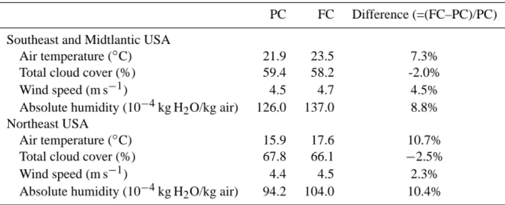
Table 1. The average value (May–Sep) for key climate variables in the surface layer (984–934 hPa) of Southeast and Midtlantic (95–65◦W
and 24–40◦N) and Northeast (95–65◦W and 40–48◦N) United States for the present climate (PC) and future climate (FC) simulations; the
last column shows the percent difference, i.e., (FC–PC)/PC, for each variable.
PC FC Difference (=(FC–PC)/PC) Southeast and Midtlantic USA
Air temperature (◦C) 21.9 23.5 7.3%
Total cloud cover (%) 59.4 58.2 -2.0% Wind speed (m s−1) 4.5 4.7 4.5%
Absolute humidity (10−4kg H2O/kg air) 126.0 137.0 8.8%
Northeast USA
Air temperature (◦C) 15.9 17.6 10.7%
Total cloud cover (%) 67.8 66.1 −2.5% Wind speed (m s−1) 4.4 4.5 2.3%
Absolute humidity (10−4kg H
2O/kg air) 94.2 104.0 10.4%
For the analyses on the severity and frequency of ozone episodes (definition provided below), we utilize 4-h aver-age surface ozone mixing ratios, 10 simulation years worth, saved over the eastern United States (105–65◦W and 24– 48◦N), corresponding to 37 model grid cells in total (pure ocean cells are excluded). We define an ozone “episode” as any occurrence, in a model grid cell, of a 4-h average sur-face ozone mixing ratio greater than 80 ppbv (the U.S. EPAs 8-h primary standard for surface ozone). Note that with the above definition there could be more than one ozone episode in a day. The 4-h averaging period corresponds to the fre-quency at which the gas-phase chemistry and aerosol mod-ules are integrated. The United States Environmental Pro-tection Agency’s (US EPA) averaging period for the primary ozone standard is 8 h. The choice of the averaging period, i.e., 4-h vs. 8-h, had a negligible effect on the number of ozone episodes.
2.5 Overview of the predicted regional climate change As discussed in Racherla and Adams (2006), it takes approx-imately three months during the six-month model initializa-tion period for the surface layer air temperatures to equili-brate to the changed ocean boundary conditions, resulting in an increase in the global annual-average values of the sur-face air temperature by 1.7◦C, the lower tropospheric spe-cific humidity by 0.9 g H2O/kg air, and the precipitation by
0.15 mm day−1. The corresponding changes in some key
ozone related meteorological variables in the surface layer (984–934 hPa) of the eastern United States are provided in Table 1. The values shown correspond to 10-year domain-averages, May through September, which we consider to be fairly representative of the “ozone season” over the United States. The spatial distribution of the predicted temperature and absolute humidity changes (not shown) compare well with other GCM’s predictions for the eastern United States provided in the IPCC TAR (IPCC, 2001). The spatial
distri-bution of the cloud cover changes (not shown) corresponds, in general, to a reduction over coastal grid cells and increases over inland cells. Based on the cloud cover changes from separate 50-year climate-only simulations, we found, how-ever, that the land-ocean cloud cover changes are not statisti-cally significant at a 95% confidence level.
2.6 Modeled ozone vs. observed: Eastern U.S.
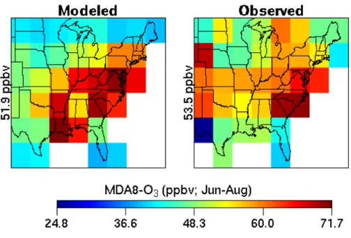
Figure 1a shows modeled (10-year average; PC simulation) and observed average maximum daily 8-h average O3
con-centrations (hereafter referred to as MDA8-O3) in the
sur-face layer of the eastern United States during the summer-time (June–Aug), while Fig. 1b shows differences between the modeled and observed summertime MDA8-O3. The
observed values correspond to much higher resolution data from the U.S. EPA’s Aerometric Information Retrieval Sys-tem (available at http://www.epa.gov/ttn/airs/airsaqs/) for the years 1993 to 2000, regridded onto the 4◦latitude by 5◦ lon-gitude grid of the model. It can be seen from Fig. 1b that the model simulates within +5 ppbv the MDA8-O3in the
north-east and midatlantic states, a region in which the observed MDA8-O3 is generally the highest. The discrepancies
be-tween the modeled and observed MDA8-O3are most
signif-icant in a few southern states (over predicts by 10–20 ppbv), wherein the natural isoprene emissions are high, and the mid-western states (under predicts by 10–20 ppbv). Although we have not investigated in further detail the mechanisms con-tributing to these discrepancies, they are likely related to the somewhat poor simulation (compared to regional-urban air quality models) of VOC-NOxlimitations, as is the case with
most global models.
We also refer the interested reader to pertinent and de-tailed studies by Fiore et al. (2002) and Fiore et al. (2003), performed using the GEOS-Chem global model of tropo-spheric chemistry (Bey et al., 2001), with which the “uni-fied” model shares a common heritage. The aforementioned
Fig. 1a. Modeled (left panel) and observed (right panel) average maximum daily 8-h average (MDA8) ozone concentrations (June–Aug) in the surface layer of the eastern United States. The modeled values (10-year average) correspond to a climate representative of the 1990s. The observed values correspond to much higher resolution data from the U.S. EPA’s Aerometric Information Retrieval System for the years 1993 to 2000, regridded onto the 4◦latitude by 5◦longitude grid of the model. In each case, the mean is displayed to the left of the panel.
White cells are pure-ocean grid cells, or those that do not have observations in them.
studies show that the GEOS-Chem model at 4◦×5◦ resolu-tion describes quite well regional high-O3events, although
the local maxima is not captured. They conclude that the GEOS-Chem model captures the synoptic-scale processes responsible for the observed temporal variability of surface O3concentrations, including high-O3 episodes. Of course,
it must be noted that the spatiotemporal resolution of the model significantly impacts the signature of urban-regional ozone episodes, leading to different results on the number, frequency and duration of ozone events than observed.
3 Results
3.1 Ozone episodes
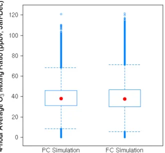
Figure 2 shows box-and-whisker plots of the predicted sur-face O3 mixing ratios in the surface layer of the eastern
United States for the PC and FC simulations. These data are not spatially averaged. The model predicts practically zero change in the spatiotemporally averaged O3mixing ratios, as
can be seen from the nearly identical surface O3median
val-ues for the PC and FC simulations. The most noticeable dif-ference between the PC and FC simulation surface O3
distri-butions, however, is in the upper extreme, wherein the model predicts a 5 ppbv increase in the 95th percentile value for the FC simulation. Racherla and Adams (2006) also previously found a small increase (1 ppbv) in the annual mean surface O3mixing ratio over the eastern United States but large
in-Fig. 1b. Differences between modeled and observed average maxi-mum daily 8-h average (MDA8) ozone concentrations (June–Aug) in the surface layer of the eastern United States. The mean dif-ference is displayed to the left of the panel. See Sect. 2.6 and the caption for Fig. 1a for details.
creases in the range of 3–9 ppbv during the summertime in the FC simulation.
Fig. 2. Box and whisker plots of the 4-h average surface layer (984– 934 hPa) ozone mixing ratios over the eastern United States (105– 65◦W and 24–48◦N) for the present climate (PC) and future
cli-mate (FC) simulations. These data are not spatially averaged; they correspond to 4-h average surface ozone mixing ratios, 10 simula-tion years worth, saved over the eastern United States, correspond-ing to 38 model cells in total (pure ocean cells are excluded). The central box shows the data between the upper and lower quartiles (25th and 75th percentile), with the median represented by a dot; whiskers go out to the 5th and 95th percentiles of the data. Val-ues beyond the 5th and 95th percentile are shown as individual data points.
The difference between the PC and FC simulations surface O3distributions is emphasized in Fig. 3, which shows
trun-cated surface O3 probability distribution functions (PDFs)
for the two simulations. The model predicts an increased probability of high-O3events in the FC simulation, with the
largest increase occurring in the 80–90 ppbv range. Recall that we defined an O3episode as any occurrence, in a model
grid cell, of a 4-h average surface O3 mixing ratio greater
than 80 ppbv (Sect. 2.4). These results show that the severity and frequency of O3episodes increases in the FC simulation.
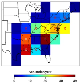
Figure 4a shows the model predicted spatial distribution of the yearly frequencies (10-year average) of O3 episodes
over the eastern United States in the PC simulation, while Fig. 4b shows the spatial distribution of the differences (FC simulation minus PC simulation) in the yearly frequencies of O3episodes. The model predicts an increased frequency
of O3episodes over most of the eastern United States, with
substantial increases of 20–40 episodes per year over some southeast and midatlantic states. We examined the statis-tical significance of the predicted changes by performing a Student’s t test upon the 10-year distributions of the yearly frequency of O3episodes in individual grid cells for the PC
Fig. 3. Probability density function of the 4-h average surface layer (984–934 hPa) ozone mixing ratios over the eastern United States (105–65◦W and 24–48◦N) for the present climate (PC) and future
climate (FC) simulations; only the upper tail (ozone mixing ratio
≥80 ppbv) of the distribution is shown here. These data are not spatially averaged; they correspond to 4-h average surface ozone mixing ratios, 10 simulation years worth, saved over the eastern United States, corresponding to 38 model cells in total (pure ocean cells are excluded).
and FC simulations. The results of the t test are also shown in Fig. 4b, wherein grid cells marked with an “X” are statis-tically significant at 95% confidence level i.e., p<0.05. It can be seen that the increases over the southeast and mi-datlantic United States are statistically significant. Collec-tively, these results show that the severity and frequency of O3 episodes over the eastern United States increases due
to climate change, with substantial and statistically signifi-cant increases occurring over some southeast and midatlantic states.
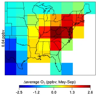
Figure 5 shows the probability of an O3 episode
occur-ring over the eastern United States duoccur-ring any 4-h period for the PC and FC simulations, January through December. We utilize the changes in O3episode probability as a surrogate
for the changes in length of the ozone season. As expected, for both PC and FC simulations, the summer months (June through August) display the highest probability for the oc-currence of O3episodes. While the largest absolute increases
occur predominantly in the summer months, it is interesting to note the larger relative increases in episode probability in the FC simulation during the fall (September/October) and spring (April/May) seasons, which, generally, have very few O3episodes under present-day meteorology and emissions.
These findings suggest a lengthening of the ozone season over the eastern United States to include late spring and early fall months. In the subsequent sections we investigate in de-tail the factors contributing to these changes.
Fig. 4a. Average yearly frequency of ozone episodes (defined here as any occurrence in a grid cell of a 4-h average ozone mixing ratio greater than 80 ppbv) in the surface layer (984–934 hPa) of the east-ern United States corresponding to the present climate simulation. White cells are pure-ocean grid cells and/or those that do not have any episodes.
3.2 Synoptic-scale circulation changes?
Some previous modeling studies (Mickley et al., 2004; Mu-razaki and Hess, 2006) have suggested that the severity and frequency of future summertime air pollution episodes in the northeastern and midwestern United States will increase due to reduced extratropical cyclone frequency in a warmer cli-mate. To investigate changes in synoptic-scale circulations over the eastern United States in the FC simulation, we ex-amined the anomalies in the daily average sea level pres-sure (SLP), May through September, over the midwest (105– 90◦W; 36–52◦N) and northeast (90–65◦W; 36–52◦N). Fig-ure 6 shows a comparison between the cumulative distribu-tion funcdistribu-tion of the daily average SLP anomaly over the mid-western United States in the PC and FC simulations, respec-tively. It can be seen that the distributions follow one another closely; the result for the northeast (not shown) is similar. The above result suggests that the simulated synoptic-scale circulations in those regions are not significantly different be-tween the PC and FC simulations. When the same analysis is performed in individual grid cells, there is up to a 4% differ-ence in the cumulative probabilities at the low-end (decrease) and the high-end (increase). Using a Kolmogorov-Smirnov test, we found that these changes are far from significant, however, as the p-values are much greater than 0.05.
Fig. 4b. Differences (future climate simulation minus present cli-mate simulation) in the average yearly frequency of ozone episodes in the surface layer (984–934 hPa) of the eastern United States. Grid cells marked with an “X” have a statistically significant (p<0.05) difference in the yearly frequency of ozone episodes, which is deter-mined using a Student’s t test upon the 10-year distributions of the yearly frequency of ozone episodes in each model grid cell for the present and future climate simulations. White cells are pure-ocean grid cells and/or those that do not have any episodes in both present and future climate simulations.
The contribution of these simulated changes in the synoptic-scale circulations to the predicted changes in O3
episodes is not clear. Regardless, our analysis (Sect. 3.3 on-wards) shows that the changes in O3 chemical production
contribute the most towards the increases in O3 episodes in
the FC simulation. In contrast to the cited earlier work, we do not find unambiguous evidence of synoptic-scale circu-lation changes driving the increase in O3 episodes. Some
possible reasons for this apparent discrepancy with previous studies are: a) the different SSTs that we utilize; and, b) the different methodology that we have employed to detect cir-culation changes, i.e., SLP anomaly distributions as opposed to a cyclone tracking method (Mickley et al., 2004).
3.3 Average ozone
Figure 7 shows the spatial distribution of the differences (FC simulation minus PC simulation) in the average (May–Sep) O3concentrations in the surface layer of the eastern United
States. It can be seen that the model predicts increases in the average O3concentrations along the relatively more
pol-luted coastal grid cells, and decreases further west. The fac-tors contributing to these changes are better understood with
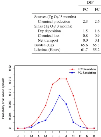
Table 2. Seasonal surface layer (984–934 hPa) ozone budget over the Southeast and Midatlantic United States (95–75◦W and 28–40◦N) for
the present climate (PC) and future climate (FC) simulations. The budget presented here is for the odd oxygen (Ox) family defined as the
sum of O3, O, NO2, 2×NO3, 3×N2O5, HNO4, HNO3, and the peroxyacylnitrates.
DJF MAM JJA SON
PC FC PC FC PC FC PC FC Sources (Tg O3/ 3 months) Chemical production 2.3 2.6 7.8 8.6 12.5 13.6 6.2 7.2 Sinks (Tg O3/ 3 months) Dry deposition 1.5 1.6 4.6 4.6 5.5 5.6 3.2 3.5 Chemical loss 0.8 0.9 2.1 2.3 3.7 4.2 1.9 2.2 Net transport 0.0 0.1 1.1 1.7 3.3 3.8 1.1 1.5 Burden (Gg) 65.6 65.3 101.9 99.7 106.5 109.3 85.9 89.1 Lifetime (Hours) 61.7 55.2 28.9 25.7 18.8 17.8 30.4 27.0
Fig. 5. The probability of an ozone episode (per model time step and grid cell) occuring over the eastern United States (105–65◦W
and 24–48◦N) for the present climate (PC) and future climate (FC)
simulations. Months J through D refer to months January through December. Monthly probabilities are calculated by normalizing the domain-wide monthly 4-h average ozone exceedances of 80 ppbv by the product of the number of grid cells (eastern United States) and simulation time steps for each month.
a surface layer O3 budget (see Table 2). We focus on the
midatlantic and southeastern states, wherein the model pre-dicts significant increases in the average O3as well as
high-O3events. The budget shown in Table 2 is actually for odd
oxygen (Ox), which is defined here as the sum of O3, O,
NO2, 2×NO3, 3×N2O5, HNO4, HNO3, and the
peroxyacyl-nitrates. It can be seen from Table 2 that two consistent fea-tures of the seasonal surface O3response to climate change
are the increased O3 chemical production (hereafter
abbre-viated as OCP) and shorter average O3lifetime. The spatial
and seasonally averaged O3 burden in the midatlantic and
southeastern states increases because, on an average, the
ef-Fig. 6. Cumulative distribution function (CDF) of the daily aver-age sea level pressure anomaly (daily spatial averaver-age minus mean) over the midwestern United States (105–90◦W; 36–52◦N) for the
present climate simulation (blue color line) and the future climate simulation (red color line). The Y-axis represents the CDF and the X-axis the daily average SLP anomaly (units of hPa).
fect of increased OCP prevails over the effect of increased O3removal rate. Further west (budget not shown) the effect
of increased O3 removal rate prevails, however, leading to
decreases in the average O3concentrations.
Table 3 provides a summary of some key factors con-tributing to increased OCP in the southeast and midatlantic United States. Increased natural isoprene emissions result in increases in the concentrations of organic peroxy radicals (RO2) and to some extent the hydroperoxy radical (HO2).
Most of the increase in HO2concentrations comes from the
increased absolute humidity alone, however. The net ef-fect of these increased peroxy radical concentrations in high-NOx regions is an increased OCP through NO+RO2 and
Table 3. Seasonal variations of a number of factors controlling ozone chemical production in the surface layer (984–934 hPa) of the Southeast and Midatlantic United States (95–75◦W and 28–40◦N) for the present climate (PC) and future climate (FC) simulations. In this
table, RO2includes peroxy radicals (lumped) formed from the oxidation of all non-methane VOCs with OH.
DJF MAM JJA SON
PC FC PC FC PC FC PC FC HO2(108molecules cm−3) 0.23 0.28 0.89 1.03 1.69 1.87 0.70 0.92
RO2(104molecules cm−3) 0.15 0.20 0.57 0.73 1.52 1.87 0.65 0.94
Isoprene emissions (Tg/3 months) 0.25 0.30 1.53 1.81 3.89 4.55 1.33 1.77 NO+HO2(Tg O3/3 months) 1.32 1.45 4.16 4.50 5.96 6.28 3.20 3.63
NO+RO2(Tg O3/3 months) 0.72 0.83 2.81 3.19 5.29 5.96 2.34 2.87 NO+CH3O2(Tg O3/3 months) 0.25 0.28 0.81 0.88 1.24 1.32 0.62 0.71
cloud cover (see Table 1) alone, in the form of increased pho-tolysis rates, contributed to the increased OCP.
The surface O3 budget (Table 2) shows that the shorter
O3lifetime during all seasons in the FC simulation occurs
through a combination of changes in the dry deposition re-moval rates, total chemical loss rates, and net transport. Note that because the burdens are different in the PC and FC sim-ulations in each season, it is important that the contribu-tion of each loss mechanism to the overall lifetime change is considered rather than the absolute change in the loss it-self. It can be seen that, with the exception of the summer months (June/July/Aug), increased dry deposition loss rates contribute most to the shorter O3lifetime. During the
sum-mer months, however, increased chemical loss rates and net transport contribute to the overall shorter O3lifetime, while
dry deposition loss rates remain nearly unchanged.
The increased chemical loss rates are due to the increases in O(1D)+H2O, O3+HO2, and O3+isoprene, as a result of
the increases in absolute humidity and natural isoprene emis-sions. The increased dry deposition removal rate during the fall, spring, and winter months is due to reduced aerody-namic and quasi-laminar sublayer resistance (RA). Because key surface parameters such as the leaf area index are be-ing held constant between the PC and FC simulations, the change in the surface resistance itself has a negligible effect. One factor that explains the reduced RAduring the aforemen-tioned seasons is the increased surface wind speeds (shown for May–Sep in Table 1), which also explains the increased net transport. We did not attempt to diagnose in further detail the changes in RA, however.
3.4 The contribution of increased natural isoprene emis-sions
In order to estimate the contribution of increased natural iso-prene emissions to the model predicted changes in surface O3over the eastern United States, we performed additional
sensitivity simulations (5 consecutive summers), with the A2 2050s climate, wherein the model evaluated isoprene emis-sions were scaled down uniformly by a factor of 1.2,
glob-Fig. 7. Differences (future climate simulation minus present cli-mate simulation) in the average (May–Sep) ozone mixing ratio (ppbv) in the surface layer (984–934 hPa) of the eastern United States. The mean difference is displayed to the left of the panel. White cells are pure-ocean grid cells.
ally. Hereafter, we refer to these simulations collectively as the FC-PISOP simulation. The factor of 1.2 corresponds to the 10-year average of the ratio of isoprene emissions in the FC to the PC simulations over the eastern United States. Note that this is a purely hypothetical modeling experiment, as it is not possible to completely separate the effects of natural isoprene emissions and climate change.
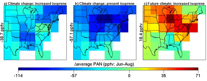
The results from the FC-PISOP simulation for summer-time O3episodes is shown in Fig. 8. This figure (and Figs. 9–
12) has three panels displaying the O3 effects of the
fol-lowing: a) climate change and increased isoprene emissions (i.e., FC simulation minus PC simulation); b) climate change alone (i.e, FC-PISOP simulation minus PC simulation); and,
Fig. 8. Differences in the summertime (June/July/Aug) frequency (5-year average) of ozone episodes (defined here as any occurrence in a grid cell of a 4-h average ozone mixing ratio greater than 80 ppbv) in the surface layer (984–934 hPa) of the eastern United States corresponding to: (a) climate change and increased isoprene emissions (i.e., FC simulation minus PC simulation); (b) climate change with present isoprene emissions (i.e., FC-PISOP simulation minus PC simulation); and, (c) future climate with increased isoprene emissions (i.e., FC simulation minus FC-PISOP simulation). White cells are pure-ocean grid cells and/or those that do not have any episodes in the simulations under comparison.
Fig. 9. Differences in the summertime (June/July/Aug) NOxmixing ratios (pptv) in the surface layer (984–934 hPa) of the eastern United
States corresponding to: (a) climate change and increased isoprene emissions (i.e., FC simulation minus PC simulation); (b) climate change with present isoprene emissions (i.e., FC-PISOP simulation minus PC simulation); and, (c) future climate with increased isoprene emissions (i.e., FC simulation minus FC-PISOP simulation). In each case, the mean difference is displayed to the left of the panel. White cells are pure-ocean grid cells.
c) increased isoprene emissions alone (i.e., FC simulation minus FC-PISOP simulation). It is evident from Fig. 8 that in the FC simulation 50–60% of the increase in summertime O3episodes over the southeast and midatlantic United States
is due to increased isoprene emissions alone. We examine next the mechanisms that contribute to the remainder of the increase.
3.5 PAN-NOxchemistry
Sillman and Samson (1995); Aw and Kleeman (2003); Daw-son et al. (2007) show that summertime O3 concentrations
increase as temperature increases, with the O3
sensitiv-ity largely driven by a decrease in the net formation of PAN, which results in increases in NOx. Changes in the
Fig. 10. As in Fig. 8 but for peroxy acetyl nitrate (PAN) mixing ratios (pptv).
Fig. 11. As in Fig. 8 but for nitric acid (HNO3) mixing ratios (pptv).
summertime NOxconcentrations are shown in Fig. 9, while
those for PAN are shown in Fig. 10. The most notice-able feature (see panels a/b of Figs. 9 and 10) is that al-though the PAN concentrations decrease throughout the east-ern United States in the FC/FC-PISOP simulations, the NOx
concentrations increase only in relatively low-O3 regions
such as the midwestern United States. This result can be explained as follows. In the high-O3regions, increased OCP
by NO+HO2/RO2in the FC/FC-PISOP simulations results in
a higher NO2:NO ratio. As a result, more NOxis present as
NO2, where it is more likely to undergo oxidation to HNO3,
and be eventually removed from the atmosphere. Evidence for this explaination, i.e., increased HNO3concentrations in
the high-O3regions in the FC/FC-PISOP simulations, is
pre-sented in Fig. 11 (see panels a/b).
The PAN increase between the FC-PISOP and the FC sim-ulations (Fig. 10c) further isolates the effect of increased iso-prene emissions on the NO2:NO ratio. That PAN increase,
in fact, points to an increase in the NO2:NO ratio, because
the steady state concentration of PAN is proportional to the NO2:NO ratio (Seinfeld and Pandis, 1998). In this case the
HNO3 concentrations decrease (see Fig. 11c), however, as
the average hydroxyl radical concentrations decrease (not shown) due to increased isoprene oxidation. These find-ings serve to illustrate the complex web of interactions that constitute the response of surface O3to climate change. In
summary, we find that the decreased PAN in the FC sim-ulation, as a result of warmer temperatures, frees up addi-tional NOx, resulting in increased OCP. At the same time,
high-Fig. 12. Differences in the summertime (June/July/Aug) ozone chemical production (105molecules cm−3s−1) by NO+HO2(5-year
aver-age) in the surface layer (984–934 hPa) of the eastern United States corresponding to: (a) climate change and increased isoprene emissions (i.e., FC simulation minus PC simulation); (b) climate change with present isoprene emissions (i.e., FC-PISOP simulation minus PC simu-lation); and, (c) future climate with increased isoprene emissions (i.e., FC simulation minus FC-PISOP simulation). In each case, the mean difference is displayed to the left of the panel. White cells are pure-ocean grid cells.
O3regions, however, the “average” NOxconcentrations
ac-tually decrease. 3.6 HOxchemistry
The FC-PISOP simulation showed that nearly half the in-crease in O3episodes in the FC simulation is attributable to
the increased natural isoprene emissions. Given the lack of unambiguous evidence linking the increase in O3episodes in
the FC simulation to synoptic-scale circulation changes, the remainder of the increase in O3episodes is also likely related
to OCP, particularly the changes in HOx. This is evident from
Table 3, which shows that upto 50% of the increased OCP in each season is due to increases in NO+HO2.
We examined the fraction of the increased OCP by NO+HO2that is due to climate change alone. This is shown
in Fig. 12. Panels a/b of this figure clearly show that the increased OCP by NO+HO2in the FC simulation is largely
due to climate change alone. Also, a comparison of Fig. 12 with Figs. 7/8 shows that, with the exception of a few grid cells, the increases in OCP by NO+HO2 coincide with the
increases in average O3 and O3 episodes. This increased
OCP by NO+HO2 is due to the increased HO2
concentra-tions associated with increased absolute humidity, and the in-creased NOxconcentrations associated with decreased PAN
(see Sect. 3.4). We conclude from these results that a sig-nificant fraction of the predicted increase in O3episodes and
average O3in the FC simulation, not associated with the
in-creased natural isoprene emissions, is due to the increases in OCP by NO+HO2.
The changes in OCP by NO+HO2merit further attention.
In the absence of increases in isoprene emissions, climate change increases the OCP by NO+HO2 over most of the
eastern United States (Fig. 12b). When isoprene emissions increase, however, the OCP by NO+HO2generally increases
in high-O3 regions and decreases in low-O3 regions. One
explanation for this behavior is that in the high-O3regions,
increased isoprene emissions promote OCP by NO+RO2and
NO+HO2whereas, in the low-O3regions, increased isoprene
emissions promotes increased radical-radical cycling (e.g. RO2-RO2, HO2-HO2, etc.).
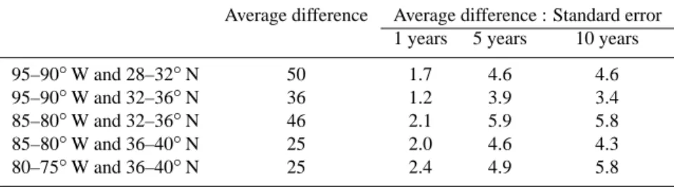
3.7 The effect of interannual variability
Our modeling shows that with only a few years (e.g. 2 years) of simulation data, it is difficult to separate the effects of interannual variability and future climate change on O3
episodes. This is illustrated in Table 4, wherein we show the 10-year average difference (FC simulation minus PC simu-lation) in the annual frequency of ozone episodes, and the ratio (ρ) of the average difference to the standard error as a function of the number of simulation years for five select locations over the southeast and midatlantic United States. For the ratio’s, the average difference is recalculated for the period under consideration, i.e., 1-year/5-year/10-year.
Utilizing the ratio ρ defined above, we can estimate the fraction (η) of the predicted change in annual O3 episodes
that could be attributed to interannual variability alone, as shown below:
η = 1
Table 4. The 10-year average difference (future climate simulation minus present climate simulation) in the annual frequency of ozone episodes, and the ratio of the average difference to the standard error as a function of the number of simulation years for five select locations over the Southeast and Midatlantic United States; for the ratio’s, the average difference is recalculated for the period under consideration, i.e., 1-year/5-year/10-year.
Average difference Average difference : Standard error 1 years 5 years 10 years 95–90◦W and 28–32◦N 50 1.7 4.6 4.6
95–90◦W and 32–36◦N 36 1.2 3.9 3.4
85–80◦W and 32–36◦N 46 2.1 5.9 5.8 85–80◦W and 36–40◦N 25 2.0 4.6 4.3
80–75◦W and 36–40◦N 25 2.4 4.9 5.8
Using Eq. (1) in Table 4 it can be seen that after 1 year η varies from 0.30 to 0.46, i.e., 30–46% of the difference in the annual frequency of O3episodes could be attributed to
inter-annual variability alone. The fraction drops to 14–20% for 5 years. It remains fairly constant thereafter. This means that with 5 years or more of simulation data, 80–85% of the pre-dicted change in the annual frequency of O3episodes could
be attributed to climate change alone. We conclude from these results that it is necessary to utilize 5 years or more of simulation data in order to separate the effects of future climate change and interannual variability on O3episodes.
3.8 Discussion
These results are associated with notable uncertainty. Firstly, the spatiotemporal resolution of the model makes it difficult to resolve accurately the boundary layer depth, VOC-NOx
limitation, and coastal-land transitions, etc. Pertinent to these modeling results is the over-prediction of surface O3
concen-trations in some southern states (see Fig. 1b and Sect. 2.6), wherein the model also predicts significant increases in O3
episodes due to climate change. Similar experiments uti-lizing regional-urban air quality models should throw more light on these results.
Secondly, the treatment of isoprene nitrates in the model, i.e., the assumed yield of isoprene oxidation by NOx, and
the assumption regarding the efficiency with which NOxis
returned to the atmosphere (see Sect. 2.2 for details), will alter the sensitivity (magnitude/sign) of surface O3 to
iso-prene emissions presented here. As an extreme case to what is currently assumed in the model, if isoprene nitrates were assumed to be a terminal sink for NOx, the increased natural
isoprene emissions in the FC simulation, acting alone, would have likely resulted in a decrease in the surface O3
concen-trations.
Finally, the predicted changes in future biogenic VOC emissions (e.g. isoprene) over specific geographical regions must also be regarded as somewhat uncertain. The first fac-tor contributing to this uncertainty is the uncertainty in cloud cover changes (see Sect. 2.4). For example, in the FC
sim-ulation, over the southeast and midatlantic United States, warmer temperatures and reduced cloud cover contributed to increased isoprene emissions. By contrast, we found that over the Mediterranean the cloud cover increased, resulting in a slight reduction in the isoprene emissions. The second factor contributing to this uncertainty is future vegetation changes, which we have not changed between the PC and FC simulations. It is worth noting here that, in addition to the uncertainties associated with future biogenic VOC sions, there is notable uncertainty in the base isoprene emis-sions distribution itself (see Fiore et al., 2005, for a detailed analysis of this issue).
4 Conclusions
We have investigated the response of surface ozone to climate change over the eastern United States by performing and an-alyzing simulations corresponding to present (1990s) and fu-ture (2050s) climates using an integrated model of global cli-mate, tropospheric gas-phase chemistry, and aerosols. Fu-ture climate is imposed using ocean boundary conditions cor-responding to the IPCC SRES A2 scenario for the 2050s decade. The predicted climate change corresponds to an in-crease in the global annual-average surface air temperature by 1.7◦C, with a 1.4◦C increase in the surface layer of the eastern United States. Present-day anthropogenic emissions and CO2/CH4 mixing ratios were used in both simulations
while climate-sensitive natural emissions were allowed to vary with the simulated climate.
Our modeling results show that the severity and frequency of ozone episodes over the eastern United States increases due to future climate change, primarily as a result of in-creased ozone chemical production. The 95th percentile ozone mixing ratio increases by 5 ppbv and the largest in-crease in the frequency occurs in the 80–90 ppbv range. The US EPA’s current 8-h ozone primary standard is 80 ppbv. The most substantial and statistically significant (p<0.05) increases in episode frequency occur in the southeast and mi-datlantic United States. We examined the extent to which synoptic-scale circulation changes influenced the increased
severity and frequency of ozone episodes by comparing the daily average sea level pressure anomaly distributions in sev-eral model grid cells for the present and future climate sim-ulations. That analysis did not provide conclusive evidence pointing to systematic circulation changes and their role in the increased frequency of ozone episodes.
These results also suggest a lengthening of the ozone sea-son over the eastern United States due to climate change to include late spring and early fall months, with increased ozone chemical production and shorter average ozone life-time being two consistent features of the predicted seasonal response of surface ozone. The increased ozone chemical production in the future climate simulation is due to increases in: 1) natural isoprene emissions, which is largest over the southeast and midatlantic United States; 2) hydroperoxy rad-ical concentrations resulting from increased water vapor con-centrations; and, 3) NOx concentrations resulting from
re-duced PAN. The shorter ozone lifetime in the future climate simulation occurs through a combination of increases in the dry deposition removal rates, total chemical loss rates, and net transport, with increased dry deposition loss rates con-tributing most to the reduced lifetime in all seasons except summer.
Changes in natural isoprene emissions may have a signif-icant effect on surface ozone levels over regions such as the southeast and midatlantic United States, where it increased annually by 20%. Our sensitivity analysis shows that higher isoprene levels account for 50–60% of the increased sum-mertime ozone episodes in the future climate simulation for that region. The model predicted changes in surface ozone due to isoprene chemistry must be treated as somewhat un-certain, however, given the uncertanties associated with the treatment of isoprene nitrates, the base isoprene emissions inventory utilized, and future changes in the influencing me-teorological factors such as cloud cover. Nevertheless, the remaining two factors causing increased surface ozone con-centrations, i.e., increased water vapor concentrations and PAN-NOxchanges, are quite robust.
These results show that there is significant interannual variability in the frequency of ozone episodes. For exam-ple, we found that after 1 year 30–46% of the increase in the yearly frequency of ozone episodes could be attributed to interannual variability alone, which, after 5 years or more of simulation data, drops to 14–20%. We conclude that it is necessary to utilize 5 years or more of simulation data in order to separate the effects of future climate change and in-terannual variability on ozone episodes in the eastern United States.
Acknowledgements. This work was supported by the NCER STAR
Program, EPA (Agreement Number: RD-83096101-0). We would like to thank R. Healy at WHOI for his help.
Edited by: R. Cohen
References
Adams, P. J., Seinfeld, J. H., and Koch, D. M.: Global concen-trations of tropospheric sulfate, nitrate, and ammonium aerosol simulated in a general circulation model, J. Geophys. Res., 104, 13 791–13 823, 1999.
Appenzeller, C., Holton, J. R., and Rosenlof, K. H.: Seasonal vari-ation of mass transport across the tropopause, J. Geophys. Res., 101, 15 071–15 078, 1996.
Aw, J. and Kleeman, M. J.: Evaluating the first-order effect of in-traannual temperature variability on urban air pollution, J. Geo-phys. Res., 108, 4365, doi:10.1029/2002JD002688, 2003. Baertsch-Ritter, N., Keller, J., Dommen, J., and Prevot, A. S. H.:
Effects of various meteorological conditions and spatial emission resolutions on the ozone concentration and ROG/NOxlimitation
in the Milan area (I), Atmos. Chem. Phys., 4, 423–438, 2004, http://www.atmos-chem-phys.net/4/423/2004/.
Bey, I., Jacob, D. J., Yantosca, R. M., Logan, J. A., Field, B. D., Fiore, A. M., Li, Q. B., Liu, H. G. Y., Mickley, L. J., and Schultz, M. G.: Global modeling of tropospheric chemistry with assim-ilated meteorology: Model description and evaluation, J. Geo-phys. Res., 106, 23 073–23 095, 2001.
Brasseur, G., Kiehl, J., Schneider, T., Granier, C., Tie, X., and Hauglustaine, D.: Past and future changes in global tropospheric ozone: Impact on radiative forcing, Geophys. Res. Lett., 25, 3807–3810, 1998.
Cess, R. D., Potter, G. L., Blanchet, J. P., Boer, G. J., et al.: Inter-comparison and interpretation of climate feedback processes in 19 atmospheric general-circulation models, J. Geophys. Res., 95, 16 601–16 615, 1990.
Chung, S. H. and Seinfeld, J. H.: Global distribution and climate forcing of carbonaceous aerosols, J. Geophys. Res., 107, 4407, doi:10.1029/2001JD001397, 2002.
Collins, W. J., Derwent, R. G., Garnier, B., Johnson, C. E., Sanderson, M. G., and Stevenson, D. S.: Effect of stratosphere-troposphere exchange on the future tropospheric ozone trend, J. Geophys. Res., 108, 8528, doi:10.1029/2002JD002617, 2003. Dawson, J. P., Adams, P. J., and Pandis, S. N.: Sensitivity of ozone
to summertime climate in the eastern USA: A modeling case study, Atmos. Environ., 41, 1494–1511, 2007.
Del Genio, A. D. and Yao, M. S.: Efficient cumulus parameteriza-tion for long-term climate studies: The GISS scheme, in: The Representation of Cumulus Convection in Numerical Models, Monogr. 46, edited by: Emanuel, K. A. and Raymond, D. J., Am. Meteorol. Soc., Boston, Mass., 181–184, 1993.
Del Genio, A. D., Yao, M. S., Kovari, W., and Lo, K. K. W.: A prog-nostic cloud water parameterization for global climate models, J. Climate, 9, 270–304, 1996.
Fiore, A. M., Jacob, D. J., Bey, I., Yantosca, R. M., Field, B. D., Fusco, A. C., and Wilkinson, J. G.: Background ozone over the United States in summer: Origin, trend, and contri-bution to pollution episodes, J. Geophys. Res, 107(D15), doi: 10.1029/2001JD000982, 2002.
Fiore, A. M., Jacob, D. J., Mathur, R., and Martin, R. V.: Appli-cation of empirical orthogonal functions to evaluate ozone sim-ulations with regional and global models, J. Geophys. Res., 108, D19 4431, doi:10.1029/2002JD003151, 2003.
Fiore, A. M., Horowitz, L. W., Purves, D. W., Levy, H., Evans, M. J., Wang, Y. X., Li, Q. B., and Yantosca, R. M.: Evaluat-ing the contribution of changes in isoprene emissions to surface
ozone trends over the eastern United States, J. Geophys. Res., 110, D12 303, doi:10.1029/2004JD005485, 2005.
Giacopelli, P., Ford, K., Espada, C., and Shepson, P.: Comparison of the measured and simulated isoprene nitrate distributions above a forest canopy, J. Geophys. Res., 110, D01 304, doi:10.1029/ 2004JD005123, 2005.
Goldstein, A., Fan, S., Goulden, M., Munger, J., and Wofsy, S.: Emissions of ethene, propene, and 1-butene by a midlatitude for-est, J. Geophys. Res., 101, 9149–9158, 1996.
Guenther, A., Hewitt, C., Erickson, D., Fall, R., Geron, C., Graedel, T., Harley, P., Klinger, L., Lerdau, M., McKay, W., et al.: A global model of natural volatile organic compound emissions, J. Geophys. Res, 100, 8873–8892, 1995.
Hansen, J., Russell, G., Rind, D., Stone, P., Lacis, A., Lebedeff, S., Ruedy, R., and Travis, L.: Efficient 3-dimensional global-models for climate studies: MODEL-I and MODEL-II, Mon. Weather Rev., 111, 609–662, 1983.
Hauglustaine, D. A., Lathiere, J., Szopa, S., and Folberth, G. A.: Future tropospheric ozone simulated with a climate-chemistry-biosphere model, Geophys. Res. Lett., 32, L24 807, doi:10.1029/ 2005GL024031, 2005.
Hogrefe, C., Lynn, B., Civerolo, K., Ku, J. Y., Rosenthal, J., Rosenzweig, C., Goldberg, R., Gaffin, S., Knowlton, K., and Kinney, P. L.: Simulating changes in regional air pollution over the eastern United States due to changes in global and re-gional climate and emissions, J. Geophys. Res, 109, D22 301, doi:10.1029/2004JD004690, 2004.
Horowitz, L., Liang, J., Gardner, G., and Jacob, D.: Export of re-active nitrogen from North America during summertime- Sensi-tivity to hydrocarbon chemistry, J. Geophys. Res., 103, 13 451– 13 476, 1998.
Horowitz, L. W., Fiore, A. M., Milly, G. P., et al.: Observa-tional constraints on the chemistry of isoprene nitrates over the eastern United States, J. Geophys. Res, 112, D12S08, doi: 10.1029/2006JD007747, 2007.
IPCC: Climate Change 2001: The Scientific Basis, Cambridge Univ. Press, New York.
Koch, D., Jacob, D., Tegen, I., Rind, D., and Chin, M.: Tro-pospheric sulfur simulation and sulfate direct radiative forcing in the Goddard Institute for Space Studies general circulation model, J. Geophys. Res., 104, 23 799–23 822, 1999.
Liao, H., Adams, P. J., Chung, S. H., Seinfeld, J. H., Mickley, L. J., and Jacob, D. J.: Interactions between tropospheric chemistry and aerosols in a unifiegeneral circulation model, J. Geophys. Res., 108, 4001, doi:10.1029/2001JD001260, 2003.
Liao, H., Seinfeld, J. H., Adams, P. J., and Mickley, L. J.: Global radiative forcing of coupled tropospheric ozone and aerosols in a unified general circulation model, J. Geophys. Res., 109, D24 204, doi:10.1029/2003JD004456, 2004.
Liao, H., Chen, W.-T., and Seinfeld, J. H.: Role of climate change in global predictions of future tropospheric ozone and aerosols, J. Geophys. Res., 111, D12 304, doi:10.1029/2005JD006852, 2006.
Logan, J. A.: An analysis of ozonesonde data for the lower strato-sphere: Recommendations for testing models, J. Geophys. Res., 104, 16 151–16 170, 1999.
Mickley, L. J., Murti, P. P., Jacob, D. J., Logan, J. A., Koch, D. M., and Rind, D.: Radiative forcing from tropospheric ozone calcu-lated with a unified chemistry-climate model, J. Geophys. Res., 104, 30 153–30 172, 1999.
Mickley, L. J., Jacob, D. J., and Field, B. D.: Effects of fu-ture climate change on regional air pollution episodes in the United States, Geophys. Res. Lett., 31, L24 103, doi:10.1029/ 2004GL021216, 2004.
Murazaki, K. and Hess, P.: How does climate change contribute to surface ozone change over the United States?, J. Geophys. Res., 111, D05 301, doi:10.1029/2005JD005873, 2006.
Racherla, P. N. and Adams, P. J.: Sensitivity of Global Tropo-spheric Ozone and Fine Particulate Matter Concentrations to Climate Change, J. Geophys. Res., 111, D24 103, doi:10.1029/ 2005JD006939, 2006.
Rind, D. and Lerner, J.: Use of on-line tracers as a diagnostic tool in general circulation model development. 1. Horizontal and ver-tical transport in the troposphere, J. Geophys. Res., 101, 12 667– 12 683, 1996.
Rind, D., Lerner, J., Shah, K., and Suozzo, R.: Use of on-line tracers as a diagnostic tool in general circulation model development 2. Transport between the troposphere and stratosphere, J. Geophys. Res., 104, 9151–9167, 1999.
Robertson, A., Overpeck, J., Rind, D., Mosley-Thompson, E., Zielinski, G., Lean, J., Koch, D., Penner, J., Tegen, I., and Healy, R.: Hypothesized climate forcing time series for the last 500 years, J. Geophys. Res., 106, 14 783–14 803, 2001.
Russell, G. L., Miller, J. R., and Rind, D.: A coupled atmosphere-ocean model for transient climate change studies, Atmos.-Ocean, 33, 683–730, 1995.
Seinfeld, J. H. and Pandis, S. N.: Atmospheric Chemistry and Physics: From Air Pollution to Climate Change, John Wiley, 3rd Ed., 1998.
Sillman, S. and Samson, F. J.: Impact of temperature on oxi-dant photochemistry in urban, polluted rural and remote envi-ronments, J. Geophys. Res., 100, 11 497–11 508, 1995. Singh, H., OHara, D., Herlth, D., Sachse, W., Blake, D.,
Brad-shaw, J., Kanakidou, M., and Crutzen, P.: Acetone in the atmo-sphere: Distribution, sources, and sinks, J. Geophys. Res, 99, 1805–1819, 1994.
Stevenson, D. S., Johnson, C. E., Collins, W. J., Derwent, R. G., and Edwards, J. M.: Future estimates of tropospheric ozone radiative forcing and methane turnoverthe impact of climate change, Geo-phys. Res. Lett., 27, 2073–2076, 2000.
Wang, Y. H., Jacob, D. J., and Logan, J. A.: Global simulation of tropospheric O3-NOx-hydrocarbon chemistry 1. Model
formula-tion, J. Geophys. Res, 103, 10 713–10 725, 1998.
Wesely, M. L.: Parameterization of surface resistances to gaseous dry deposition in regional-scale numerical-models, Atmos. Env-iron., 23, 1293–1304, 1989.
Zeng, G. and Pyle, J. A.: Changes in tropospheric ozone between 2000 and 2100 modeled in a chemistry-climate model, Geophys. Res. Lett., 30, 1392, doi:10.1029/2002GL016708, 2003.