Validation of a personalized dosimetric evaluation tool (Oedipe) for targeted radiotherapy based on the Monte Carlo MCNPX code

(1)

HAL Id: hal-03018232

https://hal.archives-ouvertes.fr/hal-03018232

Submitted on 30 Nov 2020

HAL is a multi-disciplinary open access

archive for the deposit and dissemination of sci-entific research documents, whether they are pub-lished or not. The documents may come from teaching and research institutions in France or abroad, or from public or private research centers.

L’archive ouverte pluridisciplinaire HAL, est destinée au dépôt et à la diffusion de documents scientifiques de niveau recherche, publiés ou non, émanant des établissements d’enseignement et de recherche français ou étrangers, des laboratoires publics ou privés.

Validation of a personalized dosimetric evaluation tool

(Oedipe) for targeted radiotherapy based on the Monte

Carlo MCNPX code

S. Chiavassa, Isabelle Aubineau-Lanièce, A. Bitar, A. Lisbona, J. Barbet, D.

Franck, J.R. Jourdain, M. Bardiès

To cite this version:

S. Chiavassa, Isabelle Aubineau-Lanièce, A. Bitar, A. Lisbona, J. Barbet, et al.. Validation of a per-sonalized dosimetric evaluation tool (Oedipe) for targeted radiotherapy based on the Monte Carlo MC-NPX code. Physics in Medicine and Biology, IOP Publishing, 2006, 51 (3), pp.601-616. �10.1088/0031-9155/51/3/009�. �hal-03018232�

(2)

Validation of a personalised dosimetric evaluation tool

(Oedipe) for targeted radiotherapy based on the Monte Carlo

MCNPX code

S Chiavassa1_{, I Aubineau-Lanièce}2_{, A Bitar}1_{, A Lisbona}1_{, J Barbet}1_{, D Franck}3_{, J R Jourdain}3_{, M}

Bardiès1

1 _{French Institute of Health and Medical Research, INSERM U601, 9 Quai Moncousu, 44000 Nantes,}

France

2 _{French Atomic Energy Commissariat (CEA), CEA-DRT/LIST/DETECTS/LNHB, 91191}

Gif-sur-Yvette, France.

3_{French Institute of Radiation Protection and Nuclear Safety, IRSN-DRPH/SDI/LEDI, BP 17, 92262}

Fontenay-aus-Roses Cedex, France.

Abstract. Dosimetric studies are necessary for all patients treated with targeted radiotherapy. In order

to attain the precision required, we have developed Oedipe, a dosimetric tool based on the MCNPX Monte Carlo code. The anatomy of each patient is considered in the form of a voxel-based geometry created using Computed Tomography images (CT) or Magnetic Resonance Imaging (MRI). Oedipe enables dosimetry studies to be carried out at the voxel scale. Validation of the results obtained by comparison with existing methods is complex because there are multiple sources of variation: calculation methods (different Monte Carlo codes, point kernel), geometries (model or specific) and geometry definitions (mathematical or voxel-based). In this paper, we validate Oedipe by taking each of these parameters into account independently.

Monte Carlo methodology requires long calculation times, particularly in the case of voxel-based geometries, and this is one of the limits of personalised dosimetric methods. However, our results show that the use of voxel-based geometry as opposed to a mathematically defined geometry decreases the calculation time two-fold, due to an optimisation of the MCNPX2.5e code.

It is therefore possible to envisage the use of Oedipe for personalised dosimetry in the clinical context of targeted radiotherapy.

1. Introduction

When using radionuclides in nuclear medicine for therapy, especially for radioimmunotherapy (RIT), dosimetric calculations should be made for each patient (Bardiès et al 2000). This principle has been adopted by the European directive Euratom 97/43 and put into practice in various European countries including France (implementing decree 2003-270 of the 24th March 2003 and the UK (in the Ionising Radiation (Medical Exposure) regulations 2000). Dosimetry of patients in nuclear medicine is based on the MIRD formalism (Loevinger et al 1991).

€

D (r

_k

) =

A

˜

_h

⋅ S(r

_k

← r

_h

)

h

∑

(1) where

€

D (r

_k

)

is the mean absorbed dose (Gy) in the target region rk,

€

˜

A

_h is the cumulated activity (Bq.s) in the different source regions rh and

€

S(r_k← rh) is the S factor (Gy.Bq

-1_.s-1_{) i.e. the mean}

absorbed dose in the target region rk per unit of activity accumulated in the source rh.

The spatial distribution of the activity accumulated in the various source regions is determined by quantitative scintigraphic imaging.

S factors are dependent on the geometry of the source and target regions. This geometry can be defined mathematically or sampled using digital images, using a voxel-based approach. Moreover,

(3)

depending the aim of the study, calculations can be performed for a patient model or specifically for a given patient.

In a diagnostic context, the usual dosimetric model consists of using tabulated S factors calculated for mathematical models (Snyder et al 1975, Clairand et al 2000). This approach, when applied for radioprotection, (Xu 2005), makes it possible to evaluate the effective dose delivered, or to compare the doses delivered by different radiopharmaceuticals (Liu et al 1999). Numerous mathematical reference models exist (ICRP 23 1975, Cristy et al 1987, Stabin et al 1995), but voxel-based models that can be used for dosimetric means have also been proposed (Zubal et al 1994, Caon 2004).

In order to reach the precision required for therapeutic applications, S factors specific to each patient must be taken into consideration i.e. the anatomy, composition and density of tissues, including tumours, all have to be taken into account. The currently used methods for anatomical investigation (MRI, CT scan, etc.) generate digital images composed of voxels. Compared to MRI images, CT images have the advantage of providing information concerning the electronic density of different tissues. Such information can be used for dosimetry calculations.

To our knowledge, no dosimetry approaches exist that enable mathematic modelling of the anatomy of an individual patient. The generation of mathematical models of different sizes and weights (Clairand et al 2000) would be close to a patient-specific approach although dosimetry would still be performed for a model rather than for a given patient.

The S factors calculated from anatomical images are different for each patient. The heterogeneity of the medium considered makes the calculation of S factors difficult. The commonly used method to resolve this type of problem is the use of Monte Carlo codes, which make it possible to simulate the transport of radiations and to record energy deposits in complex geometries and for heterogeneous media (that cannot be modelled analytically). There are, however, two limits to the use of Monte Carlo codes:

Firstly, Monte Carlo techniques require considerable computingresources, especially for extended geometries (whole body). Despite increases in computer capacity, the calculation time limits the application of the Monte Carlo method to dosimetry in the clinical context.

Secondly, the results obtained using Monte Carlo simulations must be validated. There are multiple sources of variation in the results:

- Different calculation approaches (i.e. different Monte Carlo codes, different methods of dealing with the interactions, different cross-sections, etc.),

- Different geometries (i.e. patient-specific vs. model)

- Different geometry definitions (voxel-based vs. mathematical definitions of organs)

An extreme example would consist of comparing S factors obtained for a patient (i.e. geometry obtained by imaging), calculated on the voxel scale by Monte Carlo simulation with S factors obtained for a mathematical model, calculated on the organ scale using a hybrid method (point kernel (Ryman et al 1987b, Berger 1968) + Monte Carlo): in this case, the differences encountered cannot be analysed in detail.

The aim of this paper is to validate our method of patient-specific dosimetry based on a Monte Carlo-type approach. Oedipe, an acronym of Tool for the Evaluation of Personalised Internal Dose, is a user-friendly graphical interface developed in IDL® _{language. Using this tool, patient anatomical}

data defined on the voxel scale from CT or MRI images can be associated with a Monte Carlo code, in this case, the MCNPX code (Hughes et al 1997). Oedipe also allows for the treatment of anatomical data and the definition of source regions on the organ or voxel scale. The simulation results are treated and displayed in the interface in the form of a list of absorbed doses by target organs, and/or isodose curves superimposed on anatomical structures when the calculation is performed on the voxel scale. We initially compared our results with those published by (Yoriyaz et al 2000) considering the same voxel-based model (Zubal et al 1994). Yoriyaz’s results were obtained using the Monte Carlo MCNP4B code (Briesmeister et al 1997), which is related to the MCNPX code used by ourselves. In a previous publication, we compared the MCNPX and EGS4 codes during a dosimetric study for the treatment of medullary thyroid cancer (Chiavassa et al 2005). Here we present a comparison with

(4)

the data published by Petoussi-Henß for a Monte Carlo code developed by the GSF laboratory (Petoussi-Henß et al 1998). In both cases, the geometries considered are similar (Zubal et al 1994). The effect of the calculation method was evaluated by comparing the S factors used by the MIRDOSE3 software (Stabin 1996) for the adult mathematical model (Cristy et al 1987) with S factors calculated directly using the Monte Carlo MCNPX code for the same mathematical model. Finally, we compared the results obtained for the same geometry (adult model by Cristy) defined differently (mathematical vs. voxel-based definition of organs). This comparison also enabled us to evaluate the effect of the voxel sampling size on the results obtained.

2. Materials and Methods

2.1. Oedipe

Oedipe is a graphical user interface that associates patient-specific anatomical data (tissue morphology, composition and density) derived from CT or MRI images (in DICOM format), with the Monte Carlo MCNPX code (Hughes et al 1997). Image processing tools have been implemented in the interface. CT images can be automatically segmented according to the 4 main densities of the human body: air [-1000 ; -800], lungs ]-800 ; -500], soft tissue ]-500 ; 400] and bone ]400 ; 1000]. Regions of interest can also be defined by manual outlining (tumours or organs of interest, MRI images). An electronic density is thus attributed to each segmented region.

The user can define the source regions at an organ or voxel scale: a cumulated activity can be attributed to each defined source region by outlining or an entry file for cumulated activity can be defined in each case for each voxel making up the anatomical image.

The entry file for the MCNPX code is created automatically from entry data. The general MCNPX Monte Carlo calculation code (Hughes et al 1997) on which Oedipe is based is an extension of the MCNP code and allows for the simulation of all particle types. The photons and the electrons are simulated between 1 keV and 1 GeV. The photon cross-sections are derived from Evaluated Nuclear Data Files (Hubbell et al 1975). The transport of electrons is derived from the ITS3.0 code (Halbleib et al 1992). Statistical uncertainty (1 sigma), proportional to

€

1/ N

(N being the number of simulated particles) is automatically estimated for each result obtained.

The MCNPX code proposes a specific format for geometry definition called ‘repeated structures’. This format is particularly well suited for voxel-based geometries as the voxel is an elementary structure that is repeated many times in the geometry. Oedipe uses the repeated structure format but MCNPX also allows for a mathematical definition of the geometry.

Once the simulation is finished, Oedipe automatically reads, processes and displays the results. The dose calculation can be carried out on the organ or voxel scale. In the case of a calculation of the absorbed dose on the voxel scale, the results are displayed in the form of isodose curves superimposed on anatomical images.

2.2. Validation a. Validation

In a previous publication (Yoriyaz et al 2000), Yoriyaz provided Specific Absorbed Fractions Φ (SAFs, kg-1) for monoenergetic photons of 0.01, 0.05, 0.1, 0.5, 1, 2 and 4 MeV and S factors (mGy.MBq-1_.s-1_{) for monoenergetic electrons of 0.935 MeV obtained with the Monte Carlo MCNP4B}

code. The geometry considered was the Zubal model (Zubal et al 1994). This is a head-torso reference model comprising 68 tissues and organs, which consists of a 3-dimensional array of 128 x 128 x 246 cubic voxels, of 4 mm on each side (Figure 1a). Yoriyaz considered bone and lungs with respective densities of 1.4 and 0.296 g.cm-3_{. The density of soft tissue (1.04 g.cm}-3_{) was considered for the rest of}

(5)

calculations were performed for the same geometry with the MCNPX code, by the intermediary of the Oedipe interface. Comparison of the results constitutes a validation of the Oedipe interface (Figure 2).

SCMS (Yoriyaz) Oedipe

Geometry Zubal Zubal

Geometry definition Voxel-based Voxel-based Calculation method Monte Carlo Monte Carlo Calculation code MCNP4B MCNPX2.5e

Figure 2: Oedipe interface validation parameters.

In order to obtain a statistical incertitude < 5%, we simulated 100000-10 million photons and 1-5 million electrons. The corresponding calculation times (CPU) are between 30 min and 4 days for photons and between 2 and 10 hours for electrons (using a 2x2 GHz G5 bi processor Power Mac). In this publication, Yoriyaz does not provide statistical uncertainty associated with the calculation, although 2-10 million simulations were carried out for photons and electrons.

b. Effect of the specificity of Monte Carlo calculation codes

Petoussi-Henß proposed Specific Absorbed Fractions (SAFs, kg-1_{) for monoenergetic photons}

of 0.03, 0.1 and 1 MeV, considering 8 source/target organs of the Zubal model (Petoussi-Henß et al 1998). The bones and lungs were considered with respective densities of 1.4 and 0.26 g.cm-3_{. The}

density of soft tissue (1.05 g.cm-3_{) was attributed to the rest of the model. These calculations were}

performed using the Monte Carlo code developed by the German National Institute for Radiation Protection (GSF). This code generates photons and monitors them individually (Veit et al 1989). The interactions under consideration in the human body are the photoelectric effect, the Compton effect and pair production. The cross-sections corresponding to these interactions are derived from the ORNL library (Roussin 1983) for simple elements. The cross-sections for the different human tissues are calculated from element data, according to the composition and density of the tissue. The energy transferred to the point of interaction is considered to be deposited locally and the secondary electron is not monitored (‘kerma’ approximation). The energy cut-off is 4 keV.

We have performed equivalent calculations for the same geometry using the MCNPX code (Figure 3). The MCNPX code monitors the secondary electrons by default and thus does not consider a local energy deposition at the point of photon interaction. We modified the MCNPX code (p and phys mode: p j 1 j) in order to apply the same approximation as the GSF code.

The statistical uncertainty associated with SAFs published by Petoussi-Henß is < 5%. Our calculations have an uncertainty of < 2% (CPU time between 30 sec. and 1,30 hours using a 2x2 GHz G5 bi-processor Power Mac).

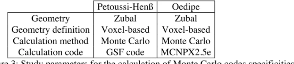
Petoussi-Henß Oedipe

Geometry Zubal Zubal

Geometry definition Voxel-based Voxel-based Calculation method Monte Carlo Monte Carlo Calculation code GSF code MCNPX2.5e

Figure 3: Study parameters for the calculation of Monte Carlo codes specificities.

c. Effect of the calculation method

The MIRDOSE3 software developed by Stabin (Stabin 1996) uses S factors calculated for the standard mathematical models developed by the Oak Ridge National Laboratory (ORNL). These

(6)

models are representative of the entire population: newborn babies, children of 1, 5 and 10 years of age, teenagers of 15 years of age, adult males (Cristy et al 1987) as well as adult females and females at 3, 6 and 9 months of pregnancy (Stabin et al 1995). These S factors are obtained for a given radionuclide based on Specific Absorbed Fractions (SAFs) Φi and mean energies Δi emitted by nuclear transition for each radiation of i type according to equation 2:

€

S(r

_k

← r

_h

) =

Δ

_i

Φ

_i

(r

_k

← r

_h

)

i

∑

(2)

The mean energies Δi emitted by nuclear transition were derived from the publication by Weber et al (Weber et al 1989). The SAFs were calculated using different methods:

- For photons (Cristy et al 1987), the Monte Carlo ALGAMP code (Ryman et al 1987a) was used with 60000 simulated particles. When the statistical uncertainty exceeded 50%, a point kernel method was used (Ryman et al 1987b), based on data published by Berger (Berger 1968). These calculations were carried out for an infinite homogeneous medium (water). However, the density of bone and lung was partly taken into account using correction factors.

- For non-penetrating radiation (electrons and beta), SAFs are usually calculated according to the MIRD formalism (Loevinger et al. 1991):

€

Φ(rk← rh) = 1/mk for self-irradiation,

and

€

Φ(rk← rh) = 0 for cross-irradiation.

In order to evaluate the effect of the calculation method on the S factors, we compared the S factors tabulated by MIRDOSE3 for the mathematical adult ORNL model (Cristy et al 1987) (Figure 1b) and iodine 131 with those calculated directly by MCNPX for the same model and the same radioelement (Figure 4). We used a mathematical geometric definition of this model in MCNPX format (Oedipe was therefore not used for geometry definition). We took all of the iodine 131 emissions (photons, electrons and beta) into consideration according to the ICRP 38 data (ICRP 1983). The sources were uniformly distributed in the 5 source organs. The maximum statistical uncertainty associated with the calculations was fixed at 5%. Ten to fifteen million particles were simulated for this purpose (CPU time between 15 and 26 hours with a 2x2 GHz G5 bi-processor Power Mac).

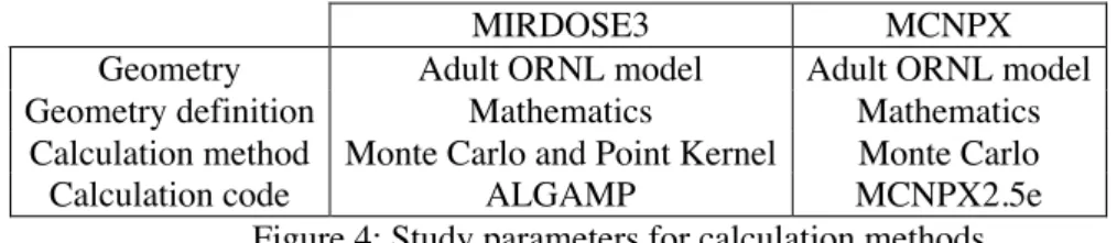
MIRDOSE3 MCNPX

Geometry Adult ORNL model Adult ORNL model Geometry definition Mathematics Mathematics

Calculation method Monte Carlo and Point Kernel Monte Carlo

Calculation code ALGAMP MCNPX2.5e

Figure 4: Study parameters for calculation methods

d. Effect of voxel sampling and voxel size

Patient anatomy is taken into account based on digital CT or MRI images. The format of these images leads to the geometry being defined by a voxel approach. In a previous publication, Peter (Peter et al 2000) compared the use of mathematical and voxel-based models for the Monte Carlo simulation of SPECT imaging. According to Peter, The voxel sampling of the geometry results in structural alterations, especially for thin or small structures. For example, closed regions can become disconnected because of voxel-sampling. The effect of such alterations becomes critical when they involve source regions. Furthermore, Peter noted errors when taking into account the course of particles arriving tangentially manner to voxel-basedsurfaces.

(7)

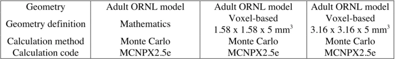
To assess the impact of using voxel-based geometry on S factor calculations, we have sampled the mathematical adult ORNL model (Cristy et al 1987) with a spatial resolution of 256 x 256 x 348 voxels of 1.58 x 1.58 x 5 mm3_{. Based on the voxel-based model, we created a second model by}

decreasing the spatial resolution to obtain a matrix of 128 x 128 x 348 voxels of 3.16 x 3.16 x 5 mm3_.

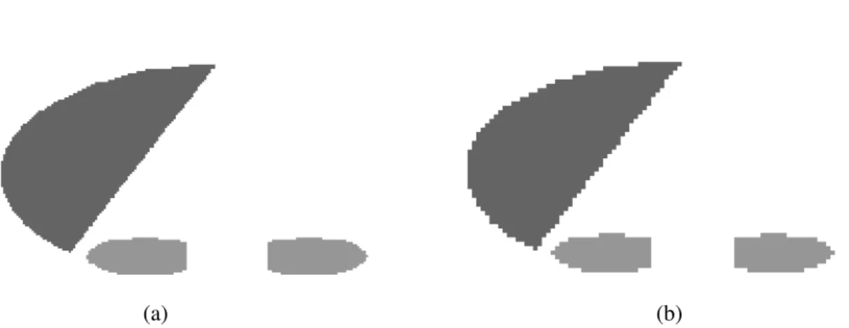
We next eliminated the slices containing only air in the 3 dimensions, so as to obtain two smaller matrices of 254 x 145 x 348 voxels (Figure 6a) and 127 x 73 x 348 voxels (Figure 6b).

Using the Monte Carlo MCNPX code, we calculated S factors (mGy.MBq-1_.s-1_{) for the}

mathematical model and the two voxel-based models (Figure 5). We simulated all iodine 131 emissions (photons, electrons and beta) according to the ICRP 38 data (ICRP 1983). The sources were distributed uniformly in 5 organs, and the calculations were carried out in 13 target organs. The maximum statistical uncertainty associated with our calculations was fixed at 5%. Ten to fifteen million particles were simulated for this purpose.

Geometry Adult ORNL model Adult ORNL model Adult ORNL model Geometry definition Mathematics Voxel-based

1.58 x 1.58 x 5 mm3

Voxel-based 3.16 x 3.16 x 5 mm3

Calculation method Monte Carlo Monte Carlo Monte Carlo

Calculation code MCNPX2.5e MCNPX2.5e MCNPX2.5e

Figure 5: Parameters to study the effect of voxel sampling and voxel size. 2.3. Calculation Times

The Monte Carlo method requires long calculation times and significant memory capacity, thus limiting the use of patient-specific dosimetric studies in the clinical context. Furthermore, according to Peter and Xu (Peter et al 2000, Xu 2005), the use of a voxel-based geometry rather than a mathematically defined approach results in a considerable increase in the memory required as well as in calculation times. However the number of simple structures (and hence interfaces) that constitute a voxel-based geometry is greater than in the case of mathematical models.

The Oedipe software is based on the Monte Carlo MCNPX code. The version 2.5e of this code was optimised in order to reduce calculation times (Hendricks 2004). This optimisation is associated with the use of a repeated structure format. Preliminary studies show that the use of the MCNPX2.5e code with repeated structures decreases the CPU time by a factor of at least 100 compared to the previous version MCNPX2.4 (data not shown). This decrease in calculation time is the result of an improvement in the calculation algorithms and is not due to variance reduction techniques.

In order to determine the impact of voxel sampling and voxel size on the amount of memory and the calculation time, we compared these parameters by considering an identical geometry (Adult ORNL model) that was either mathematical or voxel-based with 2 voxel sizes (Figure 5), following the procedure described in 2.2.d.

3. Results and Discussion

3.1. Validation

Tables 1 to 7 show the SAFs (kg-1_{) calculated by Yoriyaz using MCNP4B and our results}

using MCNPX for photons with an energy of between 10 keV and 4 MeV. The ratio between these values was generally close to 1: [0.94; 1.05] for 10 keV, [0.98; 1.12] for 50 keV, [0.97; 1.11] for 100 keV, [0.97; 1.07] for 500 keV, [0.94; 1.06] for 1 MeV, [0.94; 1.04] for 2 MeV and [0.96; 1.09] for 4 MeV. Occasionally, however, some values gave higher ratios:

- The SAF(Liver←Kidneys) values for 10 keV and the SAF(Spleen←Adrenals) values for 2 MeV gave a ratio

of approximately 20 and 0.1 respectively.

- The ratios calculated for the SAFs(Target←Lungs) at 500 keV were between 0.87 and 1.22.

(8)

The S factors calculated using MCNP4B and MCNPX for electrons of 0.935 MeV (table 8) gave ratios between 0.98 and 1.02 except for two very small values, S(Lungs←Kidneys) and S(Kidneys←Lungs).

On the whole, we achieved good concordance between the results obtained using MCNP4B and MCNPX with only a few values giving large differences. Unlike the MCNPX2.5e code, the MCNP4B code is not optimised for the decrease in calculation times, certain values published by Yoriyaz are associated with considerable statistical uncertainty (Yoriyaz, personal communication). This probably explains the occasional differences noted.

3.2. Effect of Monte Carlo calculation code specificities

In a previous study (Chiavassa et al 2005), Oedipe was compared to the Monte Carlo EGS4 code in a dosimetric study for the treatment of medullary thyroid cancer. The results obtained using the same voxel-based model (Zubal) showed variations below 10%. In this example, the EGS4 and MCNPX codes gave similar results.

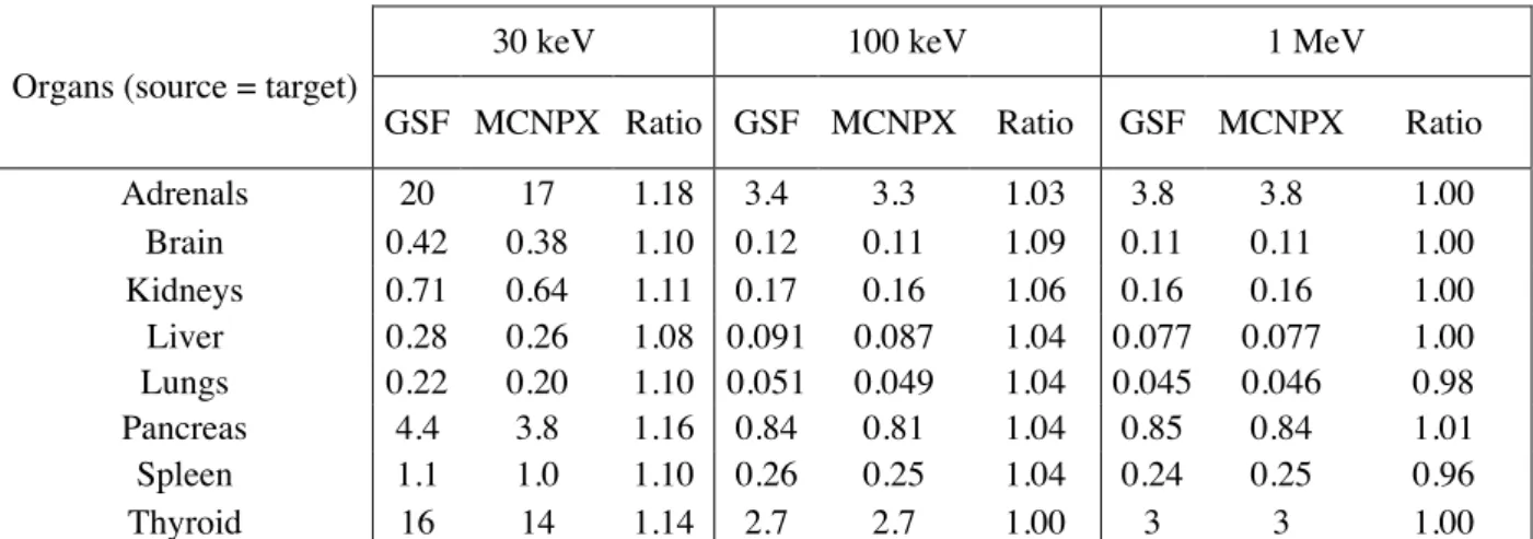
In this paper, we compared MCNPX (Oedipe) to a Monte Carlo code developed by the GSF laboratory (table 9). The ratio between the SAFs (kg-1_{) calculated using the two codes increased when}

the photon energy decreased. These ratios were less than 1.18, 1.09 and 0.96 for 30 keV, 100 keV and 1 MeV respectively. These variations can be explained by the different specificities of the two codes: cross-sections and energy cut-off (1 keV for MCNPX versus 4 keV for the GSF code). The difference between the results obtained with the GSF and MCNPX codes was thus greater than in the previous example, but can be considered as acceptable, particularly in the case of photons of 100 keV and 1 MeV.

3.3. Effect of the calculation method

The S factors integrated into the MIRDOSE3 software and those calculated by MCNPX were similar (table 10). The ratios between the values were between 0.93 and 1.06 for the organs considered, except for the skin (with a ratio of 1.10 when the source was distributed in the lungs). Moreover, the ratio between the S factors (Brain←Kidneys) was equal to 0.62. The values were nevertheless

small.

The values shown in MIRDOSE3 were obtained from Monte Carlo simulations accepting a high statistical uncertainty or a point kernel method (Cristy et al 1987), according to the calculation methods available at the time. All of the values calculated using MCNPX had an associated statistical error below 5%. It is also worth noting that the values noted for the Iodine 131 emissions come from different sources: ICRP 38 for our calculations and Weber et al. (Weber et al. 1989) for the values present in MIRDOSE3. Taking into account these large differences in the calculation methods used, the differences observed were remarkably small.

3.4. Effect of voxel sampling and voxel size

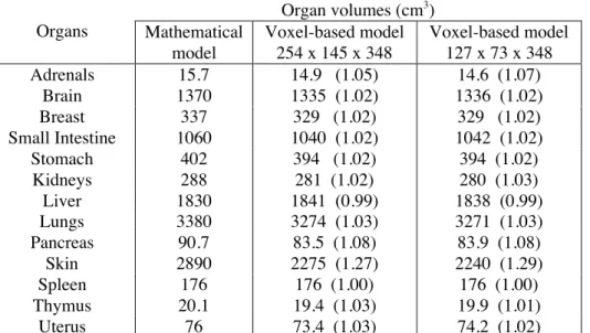
Voxel sampling of the adult ORNL mathematical model led to variations in organ volume (table 11). The ratio between the organ volumes given by the mathematical model and the voxel-based model was close to 1 (between 0.99 and 1.03) for organs that are relatively large and compact. This was more marked for small sized organs such as adrenals (up to 1.07), or elongated organs such as the pancreas (up to 1.08). As expected, the greatest variation was noted for the skin (up to 1.29) which is a thin organ. The thickness of the skin in the mathematical model is 2 mm (Cristy et al 1987).

The S factors calculated using MCNPX for the two voxel-based models are given in table 12. These values were compared to S factors calculated using MCNPX for the adult mathematical ORNL model (table 10). With the exception of the skin, the ratios between the S factors of the mathematical model and the most accurately sampled model (voxels of 1.58 x 1.58 x 5 mm3_{) were between 0.93 and}

1.08. As expected, for the voxel-based model where the spatial resolution was decreased (voxels of 3.16 x 3.16 x 5 mm3_{) the ratios were generally higher (0.93 to 1.12). The ratios between the S factors}

(9)

the lower resolution sampled model. This difference is in concordance with the differences in volume noted for the skin between the 3 models (table 11).

The effect of voxel sampling of the adult mathematical ORNL model was less critical in the results published by Peter (Peter et al 2000) where an accurately detailed cardiac mathematical model was used, which was more distorted by voxel sampling. However, it is obvious that certain thin or small organs cannot be realistically represented by a voxel-based geometry. Nevertheless, representation of individualised patient anatomy based on CT or MRI images is vital in targeted radiotherapy. Furthermore, the use of voxel-based geometries implies that a heterogeneous distribution of cumulated activity can be taken into account in source organs and absorbed doses can be calculated at the tissue level.

3.5. Calculation times

The definition of geometry in the form of voxels leads to an increase in the amount of memory necessary for Monte Carlo calculations. We performed simulations for the adult mathematical ORNL model and 2 based representations of this model. The simulations carried out for the voxel-based model with the higher resolution (1.58 x 1.58 x 5 mm3_{) and the lower resolution (3.16 x 3.16 x 5}

mm3_{) necessitated 4 and 2 fold more memory respectively than the simulations with the mathematical}

model. Compared to the mathematical model, the size of the entry files was increased approximately 50-fold for the higher resolution voxel-based model and about 25-fold for the lower resolution model (table 13).

Contrary to the studies published by Peter and Xu (Peter et al 2000, Xu 2005), in our study we found the calculation times to be approximately 2-fold lower for the voxel-based model than for the mathematical model (table 13). As expected, a mathematical definition of the geometry does not enable use of the repeated structures format related to optimisation of the MCNPX2.5e code. This example illustrates the capacity of the improvements in calculation algorithms made for this code.

4. Conclusion

Oedipe is a patient-specific dosimetric tool based on the Monte Carlo MCNPX code. Comparison of the data calculated by Yoriyaz using the same method with the MCNP4B codes constitutes the validation of this tool. The comparisons discussed in this paper validate the Oedipe software by independently taking into account the various parameters influencing dosimetric calculations.

The current Monte Carlo codes have different specificities. The two examples discussed in this paper (MCNPX/EGS4 and MCNPX/code GSF) show that the use of different codes (MCNPX/code GSF) has an impact on dosimetric calculations, but that in general the results obtained are similar. The MCNPX code is well known and widely used by the scientific community. In addition, the statistical relevance of the results obtained can be evaluated and the number of simulated particles subsequently adjusted according to the precision required.

The comparison of the results obtained by MCNPX with those integrated in MIRDOSE3 shows a striking similarity when the geometries under consideration are identical.

Oedipe enables a patient’s individual anatomy to be taken into consideration instead of having to use a standard model, with the aim of achieving the precision required for targeted radiotherapy. Taking the anatomy of each patient into account using CT or MRI images logically results in defining the geometry with the help of voxels. This format has numerous advantages. Firstly, it enables the heterogeneous distribution of the cumulated activity at the heart of the organs to be considered and the distribution of the absorbed dose in the tissue to be calculated at the tissue scale. Moreover, using this format it is possible to take advantage of the optimisation of the MCNPX2.5e code. Our comparisons show that for this code, the calculation time is 2-fold less for the voxel-based model than for the same model defined mathematically. The results obtained for the two geometrical definitions are similar except for small size organs or thin organs such as the skin. One drawback of voxel-based geometries is the size of the voxels, which limits the definition of this type of organ.

A major limitation of patient-specific dosimetric studies using Monte Carlo calculations is the excessive calculation times often necessary for this method. Oedipe uses the optimised MCNPX2.5e

(10)

code. The calculation times necessary are compatible with clinical use, thus leaving no doubt that studies of patient-specific dosimetry can be undertaken at the organ scale in the context of clinical applications of targeted radiotherapy. Dosimetric studies on the voxel scale could also be envisaged but would require longer calculation times. This limitation should be easily overcome by the use of computer networks working in parallel.

Acknowledgements

The comparisons published in this paper were made possible thanks to the invaluable data of H. Yoriyaz and N. Petoussi-Henß on their calculation methods. The mathematical definition of the adult ORNL model in MCNPX format was provided by S. Ménard and C. Furstoss of the External Dosimetry Laboratory (SDE) at the French Institute of Radiation Protection and Nuclear Safety (IRSN). The authors wish to thanks Dr. Glenn Flux for checking the manuscript.

References

Bardiès M and Pihet P 2000 Dosimetry and microdosimetry of targeted radiotherapy Current Pharmaceutical Design 6 1469-1502

Berger MJ. 1968 MIRD Pamphlet N°2: Energy deposition in water by photons from point isotropic sources. J. Nucl. Med. 1:15s-25s

Briesmeister JF 1997 MCNPTM_{- A general Monte Carlo N-particle transport code, version 4B Report}

LA-12625-M. Los Alamos, NM: Los Alamos National Laboratory

Caon M 2004 Voxel-based computational models of real human anatomy: a review Radiat. Environ. Biophys. 42 229-35

Chiavassa S, Lemosquet A, Aubineau-Lanièce I, de Carlan L, Clairand I, Ferrer L, Bardiès M, Franck D and Zankl M 2005 Dosimetric Comparison of Monte Carlo codes (EGS4, MCNP, MCNPX) Considering External And Internal Exposures Of The Zubal Phantom To Electron And Photon Sources Radiat. Prot. Dosim. 113/1-4, (8)

Clairand I, Bouchet LG, Ricard M, durignon M, Di Paola M and Aubert B 2000 Improvement of internal dose calculation using mathematical models of different adult heights Phys. Med. Biol. 45 2771-85

Cristy M. and Eckerman KF 1987 Specific Absorbed Fractions of Energy at Various Ages from Internal Photon Sources ORNL/NUREG/TM-8381/V1. Oak Ridge, TN: Oak Ridge National Laboratories

Halbleib JA, Kensek RP, Mehlhorn TA, Valdez GD, seltzer SM and Berger MJ. 1992 ITS Version 3.0 : Intergrated TIGER Series of Coupled Electron/Photon Monte Carlo Transport Codes SAND91-1634

Hendricks JS 2004 MCNPX, Version 2.5e LA-UR-04-0569

Hubbell JH, Veigele WJ, Briggs EA, Brown RT, Cromer DT and Howerton JR 1975 Atomic Form Factors, Incoherent Scattering Functions, and Photon Scattering Cross Sections J. Phys. Chem. Ref. Data 4 471-538

Hughes HG, Prael RE and Little RC 1997 MCNPX the LAHET/MCNP Code Merger XTM-RN (U) 97-012

(11)

ICRP Publication 38 1983 Radionuclide Transformations: Energy and Intensity of Emissions Annals of the ICRP 11-13. Oxford: Pergamon Press

ICRP Publication 23 1975 Reference Man: anatomical, physiological and metabolic characteristics Report of the task group on Reference Man, Oxford: Pergamon Press

Loevinger R, Budinger T and Watson E 1991 MIRD primer for absorbed dose calculations. Revised Edition New York : Society of Nuclear Medicine

Liu A, Williams LE, Lopatin G, Yamauchi DM, Wong YC and Raubitschek AA 1999 A radionuclide therapy treatment planning and dose estimation system J. Nucl. Med. 40 1151-53

Peter J, Tornai MP and Jaszczak RJ 2000 Analitical versus voxelized phantom representation for Monte Carlo simulation in radiological imaging IEEE trans. On Med. Imag. 5(19) 556-64

Petoussi-Henß N and Zankl M 1998 Voxel Anthropomorphic Models as a Tool for Internal Dosimetry Radiat. Prot. Dosim. 79 415-418

Roussin RW 1983 Description of the DLC-99/HUGO Package of Photon Interaction Data in ENDF/B-V Format ORNL/RSIC-46. Oak Ridge, TN: Oak Ridge National Laboratories

Ryman JC, Warner GG and Eckerman KF 1987a ALGAMP – a Monte Carlo radiation transport code for calculating specific absorbed fractions of energy from internal or external photon sources. ORNL/TM-8377. Oak Ridge National Laboratory

Ryman JC, Warner GG and Eckerman KF 1987b Computer codes for calculating specific absorbed fractions of energy from internal photon sources by the point-source kernel method. ORNL/TM-8378. Oak Ridge National Laboratory

Snyder WS, Ford MR, Warner GG and Watson SB 1975 “S,” absorbed dose per unit cumulated activity for selected radionuclides and organs MIRD Pamphlet n° 11. Society of Nuclear Medicine Stabin MG 1996 MIRDOSE/ Personal Computer Software for Internal Dose Assessment in Nuclear Medicine J. Nucl. Med. 37 538-46

Stabin M G and Watson EE, Cristy M, Ryman JC, Eckerman KF, Davis JL, Marshall D and Gehlen MK 1995 Mathematical Models and Specific Absorbed Fractions of Photon Energyin the Nonpregnant Adult Female and the End of Each Trimester of Pregnancy ORNL/TM-12907. Oak Ridge, TN: Oak Ridge National Laboratories

Veit R, Zankl M, Petoussi N, Mannweiler E, Williams G and Drexler G 1989 Tomographic anthropomorphic models, Part I: Construction technique and description of models of an 8 week old baby and a 7 year old child GSF-Bericht 3/89 (Neuherberg: GSF - National Research Center for Environment and Health)

Weber DA, Eckerman KF, Dillman LT and Ryman JC 1989 MIRD radionuclide data and decay schemes. The society of nuclear medicine, N.Y.

Xu G 2005 Stylized versus tomographic: an experience on anatomical modelling at RPI Monte Carlo 2005 Topical Meeting, Chattannoga, Tennessee, April 17-21, American Nuclear Society, LaGrange Park, IL

Yoriyaz H and Dos Santos A 2000 Absorbed fractions in a voxel-based phantom calculated with MCNP-4B code Med. Phys. 27(7) 1555-62

(12)

Zubal IG, Harrel CR, Smith EO, Rattner Z, Gindi GR and Hoffer PB 1994 Computerized Three-dimensional Segmented Human Anatomy Med. Phys. 21(2) 299-302

(13)

Figure 1: Voxel-based Zubal model (a) and the standard adult ORNL mathematical model (b).

(b)

(14)

(a) (b)

Figure 6: Two-dimensional voxel-based representation of the liver and kidneys of the adult ORNL model with two voxel sampling sizes: 1.58 x 1.58 x 5 mm3_{(a) and 3.16 x 3.16 x 5 mm}3 _(b).

(15)

Source organ Target

organ Method Liver Kidneys Lungs Pancreas Spleen Adrenals

MCNP4B 4,91e-1 6,44e-2 1,19e-3 2,09e-4 0 9,87e-3

Liver

MCNPX 4,91e-1 3,32e-3 1,15e-3 2,14e-4 0 9.73e-3

MCNP4B 3,25e-3 1,81 0 1,35e-2 6,18e-3 7,95e-2

Kidneys

MCNPX 3,32e-3 1,81 0 1,33e-2 6,19e-3 7.89e-2

MCNP4B 1,27e-3 0 7,51e-1 0 4,54e-3 0

Lungs

MCNPX 1,30e-3 0 7,52e-1 0 4,57e-3 0

MCNP4B 2,13e-4 1,40e-2 0 16,6 0 3,71e-1

Pancreas

MCNPX 2,13e-4 1,33e-2 0 16,6 0 3.95e-1

MCNP4B 0 6,28e-3 4,06e-3 0 2,53 0

Spleen

MCNPX 0 6,20e-3 4,07e-3 0 2,53 0

MCNP4B 9,11e-3 8,05e-2 0 3,75e-1 0 171

Adrenals

MCNPX 9,65e-3 8,00e-2 0 3,71e-1 0 171

Table 1: SAF values (kg-1_{). Photon energy of 10 keV.}

Source organ Target

MCNP4B 1.42e-1 3.00e-2 1.75e-2 3.80e-2 4.47e-3 6.09e-2 Liver

MCNPX 1.37e-1 2.92e-2 1.61e-2 3.75e-2 4.32e-3 5.98e-2 MCNP4B 3.00e-2 2.71e-1 6.19e-3 6.04e-2 5.19e-2 1.15e-1 Kidneys

MCNPX 2.87e-2 2.65e-1 5.75e-3 5.87e-2 4.99e-2 1.13e-1 MCNP4B 1.84e-2 6.50e-3 8.03e-2 1.22e-2 2.30e-2 1.37e-2 Lungs

MCNPX 1.75e-2 6.10e-3 7.79e-2 1.19e-2 2.15e-2 1.34e-2

MCNP4B 3.79e-2 5.86e-2 1.16e-2 1.38 4.56e-2 2.59e-1

Pancreas

MCNPX 3.77e-2 5.87e-2 1.14e-2 1.35 4.40e-2 2.53e-1

MCNP4B 4.38e-3 5.18e-2 2.16e-2 4.56e-2 4.30e-1 2.99e-2 Spleen

MCNPX 4.28e-3 4.96e-2 1.97e-2 4.41e-2 4.15e-1 2.90e-2

MCNP4B 5.97e-2 1.18e-1 1.41e-2 2.59e-1 3.02e-2 5.35

Adrenals

MCNPX 6.08e-2 1.20e-1 1.26e-2 2.49e-1 2.78e-2 5.29

Source organ Target

MCNP4B 9,01e-2 2,32e-2 1,42e-2 2,89e-2 5,73e-3 4,35e-2 Liver

MCNPX 8,67e-2 2,19e-2 1,29e-2 2,79e-2 5,28e-3 4,21e-2 MCNP4B 2,31e-2 1,65e-1 6,82e-3 4,36e-2 3,65e-2 7,65e-2 Kidneys

MCNPX 2,16e-2 1,62e-1 6,16e-3 4,23e-2 3,43e-2 7,48e-2 MCNP4B 1,42e-2 6,81e-3 5,02e-2 1,14e-2 1,70e-2 1,27e-2 Lungs

MCNPX 1,30e-2 6,22e-3 4,88e-2 1,07e-2 1,56e-2 1,19e-2 MCNP4B 2,88e-2 4,35e-2 1,12e-2 8,20e-1 3,54e-2 1,60e-1 Pancreas

MCNPX 2,85e-2 4,30e-2 1,10e-2 8,15e-1 3,34e-2 1,57e-1 MCNP4B 5,75e-3 3,62e-2 1,67e-2 3,51e-2 2,59e-1 2,47e-2 Spleen

MCNPX 5,25e-3 3,39e-2 1,54e-2 3,28e-2 2,51e-1 2,34e-2

MCNP4B 4,31e-2 7,55e-2 1,30e-2 1,63e-1 2,33e-2 3,34

Adrenals

MCNPX 4,05e-2 7,57e-2 1,21e-2 1,59e-1 2,39e-2 3,31

(16)

Source organ Target

MCNPX 1.15e-2 5.88e-3 4.84e-2 9.07e-3 1.40e-2 1.02e-2 MCNP4B 2.34e-2 3.69e-2 1.05e-2 8.97e-1 2.72e-2 1.51e-1 Pancreas

MCNPX 2.31e-2 3.65e-2 9.15e-3 8.95e-1 2.69e-2 1.49e-1 MCNP4B 5.19e-3 3.11e-2 1.80e-2 2.76e-2 2.63e-1 2.06e-2 Spleen

MCNPX 4.95e-3 3.05e-2 1.39e-2 2.67e-2 2.61e-1 2.00e-2

MCNP4B 3.64e-2 6.91e-2 1.32e-2 1.53e-1 1.95e-2 3.89

Adrenals

MCNPX 3.39e-2 7.12e-2 1.06e-2 1.51e-1 1.97e-2 3.90

Source organ Target

MCNP4B 7,58e-2 1,74e-2 1,07e-2 2,10e-2 4,82e-3 3,22e-2 Liver

MCNPX 7,54e-2 1,73e-2 1,06e-2 2,08e-2 4,69e-3 3,19e-2 MCNP4B 1,76e-2 1,51e-1 5,49e-3 3,34e-2 2,82e-2 6,34e-2 Kidneys

MCNPX 1,72e-2 1,51e-1 5,45e-3 3,31e-2 2,78e-2 6,33e-2 MCNP4B 1,07e-2 5,53e-3 4,25e-2 8,32e-3 1,29e-2 9,35e-3 Lungs

MCNPX 1,04e-2 5,48e-3 4,28e-2 8,22e-3 1,27e-2 9,30e-3 MCNP4B 2,10e-2 3,26e-2 8,18e-3 7,97e-1 2,41e-2 1,37e-1 Pancreas

MCNPX 2,16e-2 3,31e-2 8,64e-3 7,95e-1 2,42e-2 1,36e-1 MCNP4B 4,82e-3 2,80e-2 1,28e-2 2,46e-2 2,37e-1 1,85e-2 Spleen

MCNPX 4,79e-3 2,78e-2 1,25e-2 2,42e-2 2,36e-1 1,82e-2

MCNP4B 3,31e-2 6,22e-2 9,45e-3 1,38e-1 1,85e-2 3,20

Adrenals

MCNPX 3,13e-2 6,61e-2 9,93e-3 1,36e-1 1,74e-2 3,22

Table 5: SAF values (kg-1_{). Photon energy of 1 MeV.}

Source organ Target

MCNPX 4.28e-3 2.37e-2 1.07e-2 2.09e-2 1.89e-1 1.57e-2

MCNP4B 2.76e-2 5.51e-2 7.33e-3 1.14e-1 1.50e-2 1.95

Adrenals

MCNPX 2.71e-2 5.28e-2 7.81e-3 1.12e-1 1.56e-2 2.00

(17)

Source organ Target

MCNPX 3.72e-3 1.92e-2 8.70e-3 1.73e-2 1.34e-1 1.29e-2

MCNP4B 2.31e-2 4.25e-2 6.97e-3 9.02e-2 1.26e-2 0.90

Adrenals

MCNPX 2.35e-2 4.13e-2 6.82e-3 8.29e-2 1.31e-2 0.93

Table 7: SAF values (kg-1_{). Photon energy of 4 MeV.}

Source organ Target

organ Method Liver Kidneys Lungs

MCNP4B 7,35e-5 4,42e-7 1,76e-7

Liver

MCNPX 7,36e-5 4,52e-7 1,72e-7

MCNP4B 4,65e-7 2,72e-4 3,17e-9

Kidneys

MCNPX 4,55e-7 2,71e-4 2,52e-9

MCNP4B 1,73e-7 0 1,12e-4

Lungs

MCNPX 1,74e-7 2,52e-9 1,12e-4

(18)

30 keV 100 keV 1 MeV Organs (source = target)

GSF MCNPX Ratio GSF MCNPX Ratio GSF MCNPX Ratio

Adrenals 20 17 1.18 3.4 3.3 1.03 3.8 3.8 1.00 Brain 0.42 0.38 1.10 0.12 0.11 1.09 0.11 0.11 1.00 Kidneys 0.71 0.64 1.11 0.17 0.16 1.06 0.16 0.16 1.00 Liver 0.28 0.26 1.08 0.091 0.087 1.04 0.077 0.077 1.00 Lungs 0.22 0.20 1.10 0.051 0.049 1.04 0.045 0.046 0.98 Pancreas 4.4 3.8 1.16 0.84 0.81 1.04 0.85 0.84 1.01 Spleen 1.1 1.0 1.10 0.26 0.25 1.04 0.24 0.25 0.96 Thyroid 16 14 1.14 2.7 2.7 1.00 3 3 1.00

Table 9: SAF (kg-1_{) calculated using 2 different Monte Carlo codes (code GSF and MCNPX) in 8}

source-target organs of the voxel-based Zubal model, considering monoenergetic photons of 30 keV, 100 keV and 1 MeV.

(19)

Source Organs

Liver Kidneys Spleen Pancreas Lungs

Target Organs

M3 MCNPX M3 MCNPX M3 MCNPX M3 MCNPX M3 MCNPX

Adrenals 1.20e-6 1.19e-6 2.03e-6 2.05e-6 1.24e-6 1.27e-6 2.58e-6 2.88e-6 6.66e-7 6.29e-7

Brain 5.50e-9 5.70e-9 1.47e-9 2.39e-9 5.71e-9 6.00e-9 4.16e-9 4.34e-9 3.33e-8 3.47e-8 Breast 2.17e-7 2.15e-7 7.49e-8 7.30e-8 1.50e-7 1.46e-7 1.96e-7 1.90e-7 6.68e-7 6.77e-7

Small

Intestine 3.26e-7 3.32e-7 5.89e-7 6.01e-7 2.91e-7 2.91e-7 3.95e-7 3.83e-7 5.02e-8 5.35e-8 Stomach 4.21e-7 4.11e-7 6.93e-7 6.96e-7 2.02e-6 2.01e-6 3.42e-6 3.29e-6 3.24e-7 3.24e-7 Kidneys 8.13e-7 8.07e-7 1.17e-4 1.15e-4 1.85e-6 1.83e-6 1.40e-6 1.35e-6 1.95e-7 2.04e-7 Liver 2.12e-5 2.13e-5 8.13e-7 8.05e-7 2.14e-7 2.17e-7 1.02e-6 1.01e-6 5.44e-7 5.52e-7 Lungs 5.45e-7 5.54e-7 1.95e-7 2.07e-7 4.51e-7 4.57e-7 4.72e-7 4.77e-7 3.35e-5 3.30e-5

Pancreas 1.02e-6 1.01e-6 1.40e-6 1.36e-6 3.58e-6 3.55e-6 3.56e-4 3.51e-4 4.72e-7 4.74e-7

Skin 1.17e-7 1.14e-7 1.33e-7 1.24e-7 1.21e-7 1.13e-7 9.87e-8 9.40e-8 1.29e-7 1.17e-7 Spleen 2.14e-7 2.17e-7 1.85e-6 1.83e-6 1.93e-4 1.91e-4 3.58e-6 3.52e-6 4.51e-7 4.51e-7 Thymus 1.76e-7 1.85e-7 6.79e-8 6.88e-8 1.04e-7 1.12e-7 1.74e-7 1.84e-7 7.89e-7 7.88e-7 Uterus 1.03e-7 1.10e-7 1.98e-7 1.98e-7 9.27e-8 9.50e-8 1.23e-7 1.24e-7 2.02e-8 2.08e-8 Table 10: S factors (mGy.Mbq-1_.s-1_{) used by MIRDOSE3 (M3) and calculated using MCNPX for the}

adult ORNL mathematical model. The source of 131_{I is uniformly distributed amongst the source}

(20)

Organ volumes (cm3₎ Organs Mathematical model Voxel-based model 254 x 145 x 348 Voxel-based model 127 x 73 x 348 Adrenals 15.7 14.9 (1.05) 14.6 (1.07) Brain 1370 1335 (1.02) 1336 (1.02) Breast 337 329 (1.02) 329 (1.02) Small Intestine 1060 1040 (1.02) 1042 (1.02) Stomach 402 394 (1.02) 394 (1.02) Kidneys 288 281 (1.02) 280 (1.03) Liver 1830 1841 (0.99) 1838 (0.99) Lungs 3380 3274 (1.03) 3271 (1.03) Pancreas 90.7 83.5 (1.08) 83.9 (1.08) Skin 2890 2275 (1.27) 2240 (1.29) Spleen 176 176 (1.00) 176 (1.00) Thymus 20.1 19.4 (1.03) 19.9 (1.01) Uterus 76 73.4 (1.03) 74.2 (1.02)

Table 11: Organ volumes (cm3_{) given by the adult ORNL mathematical model and the same model}

sampled considering two voxel sampling sizes: 254 x 145 x 348 voxels of 1.58 x 1.58 x 5 mm3_and

127 x 73 x 348 voxels of 3.16 x 3.16 x 5 mm3_{. The ratios of the organ volumes given by the}

(21)

Source Organs

Liver Kidneys Spleen Pancreas Lungs

Target Organs VBM 1 VBM 2 VBM 1 VBM 2 VBM 1 VBM 2 VBM 1 VBM 2 VBM 1 VBM 2 Adrenals 1.27e-6 1.20e-6 1.99e-6 2.06e-6 1.27e-6 1.32e-6 2.94e-6 2,91e-6 6.69e-7 6.22e-7

Brain 5.58e-9 5.56e-9 2.22e-9 2.34e-9 5.86e-9 5.69e-9 4.06e-9 4.13e-9 3.56e-8 3.53e-8 Breast 2.21e-7 2.20e-7 7.32e-8 7.27e-8 1.43e-7 1.41e-7 1.88e-7 1.93e-7 6.85e-7 6.83e-7

Small

Intestine 3.45e-7 3.44e-7 6.38e-7 6.44e-7 3.07e-7 3.09e-7 4.05e-7 4.08e-7 5.52e-8 5.53e-8 Stomach 4.18e-7 4.18e-7 7.11e-7 7.11e-7 2.05e-6 2.04e-6 3.27e-6 3.24e-6 3.16e-7 3.14e-7 Kidneys 8.09e-7 8.06e-7 1.18e-4 1.18e-4 1.83e-6 1.84e-6 1.37e-6 1.35e-6 2.01e-7 2.00e-7 Liver 2.11e-5 2.12e-5 8.10e-7 8.07e-7 2.22e-7 2.21e-7 1.05e-6 1.06e-6 5.58e-7 5.61e-7 Lungs 5.63e-7 5.62e-7 2.05e-7 2.02e-7 4.41e-7 4.40e-7 4.71e-7 4.67e-7 3.40e-5 3.39e-5 Pancreas 1.07e-6 1.07e-6 1.38e-6 1.36e-6 3.47e-6 3.43e-6 3.79e-4 3.77e-4 4.70e-7 4.66e-7 Skin 1.43e-7 1.41e-7 1.42e-7 1.36e-7 1.38e-7 1.40e-7 1.14e-7 1.09e-7 1.47e-7 1.42e-7 Spleen 2.21e-7 2.19e-7 1.84e-6 1.84e-6 1.91e-4 1.91e-4 3.46e-6 3.39e-6 4,43e-7 4.36e-7 Thymus 1.80e-7 1.97e-7 6.82e-8 6.66e-8 1.13e-7 1.19e-7 1.78e-7 1.64e-7 8.00e-7 7.81e-7 Uterus 1.10e-7 1.05e-7 2.02e-7 1.97e-7 9.22e-8 9.33e-8 1.26e-7 1.22e-7 2.03e-8 2.04e-8 Table 12: S factors (mGy.MBq-1_.s-1_{) calculated using MCNPX for}131_{I and for 2 voxel-based}

representations of the adult ORNL mathematical model. Two samplings are considered: 254 x 145 x 348 (VBM 1) and 127 x 73 x 348 voxels (VBM 2).

(22)

Mathematical model Voxel-based model 127 x 73 x 348 voxels

Voxel-based model 254 x 145 x 348 voxels

Memory (Mbytes) 57 106 252

Size of entry files (Mo) 0.028 0.696 1.5

CPU (hour) 15.2 7.9 7

Table 13: Amount of memory (Mbytes), simulation entry file size (Mo) and calculation time (hours) necessary to calculate the S factors using MCNPX in 13 target organs of the adult ORNL model with a statistical incertitude less than 5% (using a G5 bi-processor Power Mac). The iodine 131 is uniformly distributed in the lungs.