HAL Id: tel-01164577
https://tel.archives-ouvertes.fr/tel-01164577
Submitted on 17 Jun 2015HAL is a multi-disciplinary open access archive for the deposit and dissemination of sci-entific research documents, whether they are pub-lished or not. The documents may come from teaching and research institutions in France or abroad, or from public or private research centers.
L’archive ouverte pluridisciplinaire HAL, est destinée au dépôt et à la diffusion de documents scientifiques de niveau recherche, publiés ou non, émanant des établissements d’enseignement et de recherche français ou étrangers, des laboratoires publics ou privés.
2D and 3D ultrafast nanoscale imaging by coherent
diffraction
Fan Wang
To cite this version:
Fan Wang. 2D and 3D ultrafast nanoscale imaging by coherent diffraction. Optics [physics.optics]. Université Paris Sud - Paris XI, 2014. English. �NNT : 2014PA112226�. �tel-01164577�
UNIVERSITÉ PARIS-SUD
ÉCOLE DOCTORALE 288 :
ONDES ET MATIÈRE
Laboratoire : LIDYL, IRAMIS, DSM, Commissariat à l’Energie
Atomique, Saclay, France
THÈSE DE DOCTORAT
PHYSIQUE
par
Fan WANG
Imagerie nanométrique 2D et 3D
ultrarapide par diffraction cohérente
Date de soutenance : 25/09/2014
Composition du jury :
Rapporteurs : M. Philippe ZEITOUN LOA-ENSTA
M. Milutin KOVACEV Universität Hannover
Acknowledgement
Firstly, I’d like to express my gratitude to my Ph.D supervisor, Dr. Hamed MERDJI. Without his reception and help for my thesis work, I couldn’t have chance to enter in fundamental research field and finish my work and thesis manuscripts at last. During the period of thesis, he offered me the greatest advice both on the research direction and moral support. He played well as a guide for my research carrier. At the same time, he helped me also to collaborate and communicate with other worldwide famous research group for deeper scientific comprehension and progress in the corresponding Ph.D subject research domain.
Then, I am also thankful to my dear colleagues in the same team: Willem Boutu, David Gauthier, Xunyou Ge, Aura Ines Gonzalez and so on, for their fruitful discussion and help on the scientific and technical comprehension in both physical theory and experience. Especially, they give me much support about the research idea, installing the experience set-up and establishing research plan and method. In this context, some experimental results during my thesis are issue from our collective diligent work. And I have learned and acquired a lot from them in both the precious scientific knowledge and attitude.
Thirdly, I never forget my family, my dear parents, and my little brother. They give me warm and love in my heart, which assurances my peaceful and concentrated long time research work. They are my heart bay, my source of fighting. Another future member, my boyfriend, who is a mathematic Ph.D candidate, gives me also important support that helps me go across the life darkness and difficulty period in writing thesis.
Last, I give also my thanks to Bertrand Carré, our group leader. He permitted me to develop research in the Attophysique group. And sometimes he supported our experience work very late at night for the laser beam. He occupied as a permanent staff on turning off the laser beam. I shall also thank my colleagues in the group but with research in other topics: Pascal Salière, Thierry Ruchon, Nan Lin et Antoine Camper, Sebastian, Elisabeth English and so on for their generous introduction and share about knowledge food. We have participated in so many seminars, summer schools for further understanding in the research for atto- or femto- laser development.
Anyway, there are still so many staffs when I met during my thesis work: our technical support colleague, Marc Billon and other staff from laser beam lime operation team: Olivier
Gobert, Benoît Mahieu
and so on. I honor them with a thankful heart.Contents
Introduction ... 4
Motivation and outline... 7
Chapter I - Principle of lens-less imaging ...
11
I.1 Few basics in lens-less imaging techniques ... 11
I.2 Image formation in lens-less imaging ... 14
I.3 Reconstruction: Phase retrieval algorithms ... 21
I.4 Reconstruction: FTH and HERALDO ... 24
I.5 Beam requirements for lens-less imaging ... 27
I.6 Conclusion ... 28
Chapter II - High harmonic generation ...
29
II.1 Introduction ... 29
II.2 Experimental set-up ... 31
II.3 HHG optimization and beamline standardization ... 34
II.4 Laser Modal Filtering for HHG optimization ... 44
II.5 Conclusion ... 48
Chapter III -Coherent Diffractive Imaging and Holographic imaging ... 51
III.1 Introduction ... 51
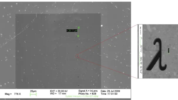
III.2 Sample preparation ... 51
III.3 Detection of the diffraction pattern ... 53
III.4 Implication of the spatial coherence in the CDI reconstructions ... 54
III.5 Experimental results of CDI ... 57
III.6 Experimental results of Fourier Transform Holography... 60
III.7 Experimental results of holography with extended reference ... 64
III.8 Signal-to-noise ratio (SNR) analysis ... 66
III.9 HERALDO reconstruction and noise ... 69
III.10 CDI reconstructions of HERALDO objects ... 88
III.11 Conclusion ... 91
Chapter IV - Towards single shot 3D Coherent Imaging ... 93
IV.1 Introduction ... 93
IV.2 Basics in three dimensional coherent imaging ... 94
IV.3 CDI reconstruction algorithm in 2D and 3D ... 98
IV.4 The ankylography : a 3D single view imaging technique ... 101
IV.5 First experimental data at the CEA HHG beamline ... 106
IV.6 Conclusion ... 119
Introduction
How is an image formed? Do we really need lenses to generate an image? Obviously, this is not necessary. The philosopher Mo Jing in ancient China, during the 5th century BC, mentioned the effect of an inverted image forming through a pinhole. Nowadays, it is still a well-applied technique but limited by the shape and size of the pinhole. What technique would overcome any manufacturing limitation? Modern optics brought the answer with diffraction and Fourier optics. Since the advances made in the last decades with the introduction of lensless imaging techniques with X-rays and particles, imaging science has witnessed extraordinary advancements. We are concerned about elucidating structural changes over broad time scales (attoseconds to many seconds) and length scales (nanoscale to macroscale). This is of interest not only in biology, but also in physics, medicine and in order to create the revolutionary materials required for future communication and energy technologies. Scientific and industrial innovations depend on our capacity to design, observe, control matter at these various space and time scales. Improved or entirely new characterization tools increase our understanding of the ‚real‛ world, from complex organized systems to a single particle. While various forms of microscopy (TEM, SEM, AFM, STM, etc.) can furnish detailed information about morphology, size, and on occasion the composition of nanoparticles, none are capable of providing real– time, on–line information.
To bridge the gap between conventional diffraction and microscopy, and to image single non-periodic objects with atomic/nanometric spatial resolution, coherent diffractive imaging (CDI) has demonstrated very high potential. Since its demonstration [1-2], many researchers have taken a large step in this direction using synchrotron radiation, free electron laser or high harmonic generation [3-8]. The idea of CDI came from the successful crystallography diffraction methods. David Sayre first raised this question that whether a similar diffraction method could be applied to non-periodic objects in 1952 [9]. J.R. Fienup proposed a phase-retrieval algorithm to solve the phase problem in 1978 [10]. His algorithm is a modified version of Gerchberg-Saxton algorithm that is originally inspired from ideas used in electron microscopy [11]. For more details of the historical development of the phase-retrieval algorithm, please refer to the review of Henry Chapman and Keith Nugent [12]. Exploiting coherence in diffraction, scientists have now in hand a revolutionary imaging system, an ultimate microscope that can see inside our ‚ultrasmall‛ world
with incredible clarity. No lens is needed, it is only necessary to record the intensity of the diffraction pattern that emerges after its interaction with the object on a high-resolution high dynamic range pixelated detector. The diffraction patterns in no way resembles the object itself, but a computer can convert this digitized diffraction pattern using a calculation known as a "phase-retrieval" to extract the information. In this way, it is possible to make much better images than with conventional lens-based systems. The spatial resolution can be pushed down to the theoretical diffraction-limit given by the source wavelength so that potentially atomic vision could be available using coherent hard X-rays.
In-situ images of individual sub-micrometer particles and molecules at atomic/nanometre resolution in their native environment can be applied to resolve both static and dynamic structures. The dream experiment would consist in producing the best-ever pictures of individual atoms, molecules or cells in any structure even if it is not crystalline.A first example is given by images of viruses recently obtained at the LCLS free electron laser (see fig. below) [13]. This is of strong interest as a big gap exists in the knowledge of viruses structures in the range from about 30nm to 500nm (see figure below). In fact, these length scales remain uncharted territory for many other biological systems.
First results from the LCLS where single mimivirus particles were injected into the FEL beam. Recorded diffraction patterns (left) and image reconstruction of the virus (right).
Third generation synchrotrons has also given extraordinary pictures, like the 3D structural image of a single nanocrystal [14] or a bone [15], ultrafast coherent X-ray flashes provided by free electron lasers (FEL) and high laser harmonic (HHG)
to understanding primary biological or chemical reactions. Ultrafast lensless imaging can be applied to follow in real time nanoscale processes; crystal stress, nano-magnetism or nanoscale phase transitions are few examples. In nano-magnetism, this will offer new tools to create and optimize next generation ultrafast storage and calculator devices.
Those illustrations are non-exhaustive and new horizons are opened. Indeed, new concepts in imaging have always fascinated mankind while creating significant economic impact. We can cite for example the extraordinary adventure of Stanford researchers transforming light field and Fourier technology from a scientific theory into a reality for everyone (https://www.lytro.com/ ).Lensless imaging has a similar potential. Why not a digital lensless camera?
CDI is a powerful tool in many scientific areas ranging from biology to solid-state physics. The key words for CDI are ‚coherence‛ and ‚diffraction‛. Indeed, the technique uses the measurement of a far field diffraction pattern to retrieve the spatial
amplitude and phase of a real space object. The large-scale facilities – synchrotron light
sources and FELs provide a large amount of photons promising a good signal-to-noise ratio in CDI. The high coherence of FELs and synchrotrons (using a pinhole in this case) ensures that the important phase information can be well ‚written‛ in the detected diffraction pattern. Moreover, the femtosecond pulse duration of FEL sources promises a bright future for ultrafast dynamic imaging at a nanometer or sub-nanometer scale.
FLASH in Hamburg (VUV FEL) LCLS in Stanford (X-ray FEL)
However, these large-scale facilities cost expensive resources and have limited access beam time. These constraints limit the wide spread of ultrafast coherent diffractive imaging. The applications are then restricted. This limits the impact of this research for example in the optimization of ultrafast nanoscale devices in communication, medicine or even in more industrial environments. Therefore, an inexpensive source
would provide a very interesting alternative: high-order harmonic generation (HHG) sources can provide intense highly coherent soft X-ray photons with ultrafast pulse duration. The relatively small size and low cost of such light source makes the HHG source an ideal alternative to synchrotrons and FELs. Up to recently, the limited brightness of HHG source was a key limitation for a table-top application of CDI. However in 2007, Richard Sandberg and colleagues have succeeded in demonstrating CDI using a kHz table-top laser driven HHG source with a spatial resolution of 214nm [7]. The brightness of the harmonic beam was still limited, and the exposure time of this experiment was on the scale of an hour (up to 106 laser shots!) that is far from reaching single shot ultrafast nanoscale imaging, required in many dynamical studies. In 2009, our research group at CEA (Commissariat à l’Energie Atomiqueet aux Energies alternatives) has demonstrated the first single-shot CDI using a table-top femtosecond soft X-ray laser harmonic source [8]. An isolated test nano-object was reconstructed with 119nm spatial resolution in a single 20fs-long shot. A spatial resolution of 62 nm was obtained from multiple laser shots (40 shots). In this context, I have joined the AttoPhysique group of CEA as a PhD student of Dr. Hamed Merdji in 2010.
Motivation and outline
The principle objective of this work is to perform extended developments and applications of ultrafast coherent imaging techniques using table-top harmonic source. I present all the efforts, either on the source, and the imaging techniques to build a reliable and powerful ultrafast microscope with nanometer spatial resolution and femtosecond temporal resolution. I present then a characterization of magnetic nano-domains at a sub-100nmscale in a single femtosecond shot. This illustrates the potential of our table-top harmonic beamline for various scientific research areas such as material science, biology and chemistry.
This work is presented in five chapters.
lens-should give a clear description of CDI and help to understand the ideas and methods used in the following chapters.
The main work and experimental results are presented respectively in Chapter 2, 3 and 4.
Chapter 2 starts with the description of the experimental setup – the table-top high flux harmonic beamline at CEA Saclay. The first step of this thesis work has been a complete optimization of the harmonic beam line from the very beginning of the infrared pump laser to the focusing optics at the end of the imaging setup. The optimization processes and results are presented in Paper I and Paper II attached to this chapter. The first one discusses the optimization of infrared pump laser using a modal filtering hollow core fiber, which leads to improvement of the HHG efficiency and stability. After the beam line optimization, spectrum and far field studies of HHG in two different gas mediums (argon and neon) are presented. The first one shows the optimization of the HHG and the diffraction stages. The objective has been to increase the photon flux, the coherence and the wave front quality of the harmonic beam. Statistic studies using a Hartmann wave front sensor and Young double slits to characterize the wave front and the coherence show the improvement of the harmonic beam and the influence of these beam properties in the image reconstruction quality. This chapter concludes with the summary of the optimized high flux harmonic beamline and a short discussion of a comparison between large-scale facilities sources (synchrotron and FELs) and table-top harmonic sources for coherent imaging.
Chapter 3 presents the second step of the thesis work: the validation of different coherent imaging techniques at the table-top harmonic beam line. It starts with experimental results of classic CDI and discussion of the spatial coherence implementation in the reconstructions. The second part is the experimental results of Fourier Transform Holography (FTH), which is a complementary imaging technique to CDI. The limitation in spatial resolution in FTH inspired several new imaging techniques such as Holography with Extended Reference by Autocorrelation Linear Differential Operation (HERALDO). HERALDO offers an alternative way for ultrafast nanometric imaging, which is easy to implement on all kinds of beam line performing coherent imaging. The step-by-step analysis of the HERALDO reconstruction process leads to a discussion of the influence of reference design and the noise ratio issue, which is reported in Paper III. Indeed, the signal-to-noise ratio gives restrictions in both CDI and holographic techniques for our experiments. A comparison between CDI, FTH and HERALDO techniques concludes this chapter.
Chapter 4 is the last achievement of this thesis work: the extension of 2D coherent diffractive to 3D. I present the theoretical study of three-dimensional coherent diffractive imaging. Generally, to accomplish a full 3D display, multiple views of objects are required. It is worthwhile to discuss the relationship between two dimensional and three dimensional diffraction imaging. Recently, a new 3D imaging technique, named ankylography, proposed to exploit high angle, single view, 2D diffraction to recover 3D amplitude and phase information. Before investigating the 3D image reconstruction process of an object from its diffraction pattern, some basic points in the 2D case are reviewed. We recall the numerical algorithm image reconstruction from a coherent diffraction pattern. In addition, we explain the numerical developments that play an important role as a bridge from 2D to 3D perception. Then we present our first experimental data and image reconstructions. Those data allow identifying restrictions in the 3D ankylographic image reconstruction.
Chapter 5 draws the perspectives and gives the general conclusion of this thesis. I summarize the main conclusions of the harmonic beamline investigations, the 2D coherent imaging techniques (CDI, FTH, HERALDO) and the first 3D imaging results. Furthermore, we open a new perspective towards 3D coherent imaging using a technique based on the stereo vision. In this configuration, 2D stereo images can be either reconstructed using coherent diffractive or holographic techniques.
Chapter I - Principle of lens-less imaging
I.1 Few basics in lens-less imaging techniques
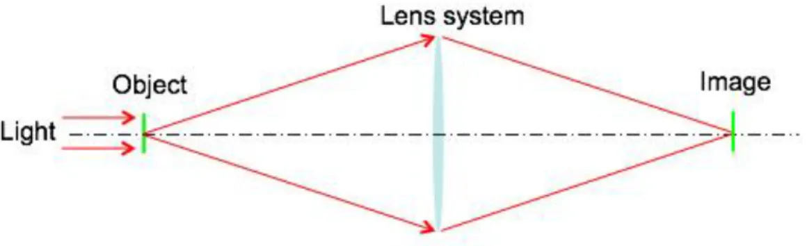
In conventional imaging systems, such as optical microscope and photo camera, a simple lens or a group of convex and/or concave lenses are used to form the image of the target object that is illuminated by a proper light source (Fig. 1.1). In complicated imaging systems, the lens system can also contain other optical elements, such as mirrors, windows, etc. The image quality is generally limited by the lens system: the ensemble of each optic’s aberration determines the possible alterations of the object image. This imposes strong constraints on manufacturing of optical elements and design of lens system. In X-ray microscopy, the highest spatial resolution to date has been obtained using zone plate Fresnel optics. The constraints on optical elements become more critical. First, the resolution of such image-forming optics is limited by the smallest outer feature of the zone plate, which raises a real challenge on the optics manufacturing if one would like to reach nanometric resolution. Secondly and more fundamentally, the material of such optics has strong photon absorption, which limits its efficiency to typically less than 10% and often as low a percent [1]. The latter one is critical for high resolution imaging of certain specimens that are sensitive to radiation damage [2,3]. In this context, the lens-less imaging provides an alternative solution for high resolution imaging for various applications from biology to solid-state physics.
Fig 1.2.Scheme of a lens-less coherent imaging set-up. The computation algorithms replace the lens system conventionally used to image the object.
In the Fraunhofer diffraction regime, the diffraction pattern is proportional to the Fourier transform of the exit wave in the image plane. Theoretically, a simple inversion of the diffraction pattern should give the image of the object. But the pixel-array detector is only sensitive to the intensities of the electromagnetic wave field. Therefore, the phase information of the wave field is not directly measured by the detector. Infinity of possible solutions of the simple inversion can be obtained by applying possible phases to the measured diffraction pattern [4]. Here comes the famous ‚phase problem‛, which is the main obstacle to extract object information from the measured diffraction pattern. Two main techniques have been proposed to overcome the ‚phase problem‛: one uses Phase Retrieval Algorithms *6,7,8+ and is called Coherent Diffractive Imaging (CDI); the other is Fourier Transform Holography (FTH) [5].
In CDI, iterative algorithms converge to the spatial phase in the diffraction plane using constraints both in real and reciprocal space (the diffraction plane). A scheme of the CDI technique is shown in Fig. 1.3. In the reciprocal space, the diffraction pattern recorded by the detector is equal to the absolute squared value of the Fourier transform of the exit wave. In the real space, the object is contained in a finite dimension (called ‚support‛). The autocorrelation defined as the Fourier transform of the measured diffraction pattern will give a first constraint to the support (other constraint can be found). The relation of Fourier transform links these two constraints between real and reciprocal spaces. In general, most phase retrieval algorithms use these two kinds of constraints to reconstruct the ‚lost phase‛ in the reciprocal space and the object image in the real space. During the detection of the diffraction patterns, the coherence of the incident wave plays an important role. It creates a characteristic ‚speckle pattern‛ in the diffraction plane. The ‚speckle‛ is the ‚phase signature‛ of the diffraction pattern that ensures the convergence of iterative algorithms. The phase retrieval algorithms reconstruct simultaneously the phase in
reciprocal space and the object image in real space. The solution is nearly unique for problems that have more than one dimension [9,10].
Fig. 1.3. The scheme of CDI can be separated into two steps: the first one is the detection of the object’s diffraction pattern. The second step is to use phase retrieval algorithms to reconstruct the ‚lost phase‛ of the diffraction pattern and the object image.
Fourier Transform Holography (FTH) is another lens-less imaging technique, which has almost the same experiment setup as the CDI except that the sample geometry holds a holographic reference. The principle of FTH is similar to holography proposed by Dennis Gabor in 1948 *11+. The FTH is inspired by this idea of ‚full recording‛: the incident wave is simultaneously diffracted by the object and the reference. The detector located in the far field records the interference between these two diffracted waves, which is called ‚hologram‛. The spatial amplitude and phase of the object are encoded in this hologram and a simple Fourier transform is required to reconstruct the object image [12] (Fig. 1.4). The Fourier transform of the hologram is the autocorrelation of the sample (object + pinhole). The reconstructed object image is the correlation between the object and the pinhole.
delta functions (which correspond to the sharp features at the edges of the extended references). Note that the Fourier transform properties of delta function ensure a high-resolution reconstruction (Fig. 1.4). By this way, the resolution is no longer limited by the reference size, so one can increase the diffraction signal without affecting the resolution. Theoretically, the reconstruction resolution is limited by the quality of the manufactured references. In particular the sharpness of the edges is crucial.
Fig. 1.4.Scheme of FTH and HERALDO: We have used the same experimental setup as in CDI except the sample geometry. In FTH, the sample consists in the object and a pinhole reference in the nearby at a distance that respects the holographic separation given by the size of the object. In HERALDO, the arrangement is similar but the reference is large while keeping the holographic separation. The reconstruction step is simple and direct: in FTH, the Fourier transform of the hologram gives the object image; in HERALDO, a linear differential operation is applied as a post process of the Fourier transform to finally get the object image reconstruction.
I.2 Image formation in lens-less imaging
The image formation is the fundamental of lens-less imaging and all ideas of reconstruction techniques are based on it and inspired by its properties. As mentioned before, CDI, FTH and HERALDO have the same experimental setup. The image formation is thus the same for these techniques from the incident wave propagation to the Fraunhofer diffraction process, except that different sample preparation for CDI and FTH/HERALDO leads to different diffraction patterns. Since the wave propagation and Fraunhofer diffraction are well known, I present here the relevant equations, formulas and properties in the case of the lens-less imaging to give a clear description of theoretical background with non-exhaustive mathematics. One can refer to the books of J.W. Goodman and to the Born and
Wolf[12,13] for detailed mathematical and physical deduction of wave propagation and Fraunhofer diffraction in general case. More practically, one can also look at some excellent thesis work such as P. Thibault [14], M. Guizar-Sicairos[15] or D. Gauthier at Saclay [16] that have well-detailed mathematical presentations of the image formation in the case of lens-less imaging.
I.2a Image formation in lens-less imaging: Diffraction
We usually consider in lens-less imaging an isolated object illuminated by a plane wave (Fig. 1.5). The exit wave is the wave field transmitted by the object and detected in the far field (by a CCD camera in our case). The propagation of the exit wave behaves according to the Helmholtz wave equation:
(Eq. 1-1)
where and . ω is the frequency of the wave ; and are respectively the electric permittivity and the magnetic permeability of the medium.
(Eq. 1-3) Obviously, unless , which is called the ‚Ewald sphere‛ *18]. In our lens-less imaging experiments, the detection plane is a plane transverse to the wave propagation direction. Thus we can separate the free-space propagating wave field into transverse and parallel components, respectively and . The general solution of Eq. 1-1 is then obtained in Fourier space as follow:
(Eq. 1-4)
where (Fig. 1.9) and are two independent functions
representing forward (+) and backward (-) scattering. In our experiments, back-propagating terms can be neglected, therefore the solution is:
(Eq. 1-5) From Eq. 1-5, we can deduce the wave function in far field diffraction (Fraunhofer diffraction) [19]:
(Eq. 1-6)
Since (far field), the integrand will not disappear unless the phase term is stationary, which means:
(Eq. 1-7)
Therefore, we can get the measured intensity by the detector in the far field:
(Eq. 1-8)
In our experiments, Eq. 1-6 can be simplified in the case of small-angle scattering (Fig. 1.6), which is valid when:
Fig. 1.6.Representation of the wave vector and the diffraction angle relationship in the Ewald sphere.
Applying the paraxial approximation, one can expand to the first non-zero order in , and Eq. 1-5 becomes
(Eq. 1-10)
One gets the small angler scattering version of Eq. 1-8:
(Eq. 1-11)
Note here that the Fraunhofer diffraction approximation is valid when the Fresnel number , which is defined as
(Eq. 1-12)
where is the characteristic dimension of the object. Small and large Fresnel numbers correspond to respectively the far field regime and the near field regime. In the Fraunhofer diffraction regime (far field), one should have
As shown in Eq. 1-11, the measured diffraction pattern is proportional to the absolute value of the Fourier transform of the exit wave in the transverse plane. The question now is: what is the relation between the object image and the exit wave that we can reconstruct by computational algorithms? For our experiments, we use the projection approximation: the exit wave is the product of the incident wave and the object transmittance:
(Eq. 1-14)
In this approximation, the object can be treated as a two dimensional plane whose thickness is negligible, thus there is no diffraction inside the object. The object transmittance (in two dimensions with complex values) represents the projection of the object on a transverse plane (object plane in Fig. 1.5), which shows how the object modifies the incident wave both in amplitude and in phase. Since we assume that the incident wave is a plane wave, the detected wave (diffraction wave) in the far field is then equal to the Fourier transform of the object transmittance. The reconstruction image that we get by computational algorithms should then reflect the object transmittance. To valid the projection approximation, the object should be ‚optically
thin‛. If is the object thickness and is the reconstruction resolution that we want to attend, then the ‚optically thin‛ condition can be described as
(Eq. 1-15)
The term describes the ‚depth of focus‛ (DOF), which is also a function of diffraction angle :
(Eq. 1-16)
When the object thickness is smaller than the DOF, the exit wave is associated to a single object plane, which corresponds to the reconstruction plane visualized with computational algorithms. Otherwise, there will be more than one object plane, thus more than one possible phase associated to the measured diffraction pattern. This can prevent convergence of iterative algorithms. One may need additional constraints on the object support to associate one and only one object plane for the reconstruction. In holographic experiments (FTH, HERALDO), the phase information is encoded in the hologram. Thus, there is one unique solution obtained in the plane of the object and the reference.
To conclude, in our lens-less imaging experiments, objects are ‚optically thin‛ and the diffraction wave is detected in the far field regime (Fraunhofer diffraction) in the small angle scattering regime.
I.2c Image formation in lens-less imaging: Detection
The detection of the diffraction pattern is realized by a CCD camera, which accumulates incoming photons (diffraction and noise) during the exposure time. Thus temporal information such as the phase of the wave function is lost during the detection. This is the phase problem well known in lens-less imaging. The measured term is the photon flux, whose unit is or . Eq. 1-11 becomes (if we omit the constant factors)
(Eq. 1-17)
The measured diffraction signal ( ) is then digitalized with a certain sampling ratio. We can use a discrete Fourier transform function to present the numerical data. The one-dimensional discrete Fourier transform of a long vector is
(Eq. 1-18)
If a continuous function is sampled by a sampling interval , and its discrete Fourier transform is also sampled by a sampling interval , then we have the following relation:
(Eq. 1-19)
(Eq. 1-21)
where is the pixel size of the CCD camera which contains X pixels, and is the pixel size of the autocorrelation of the object transmittance. If the object transmittance occupies a region of X pixels in the matrix of X pixels and the object size is X , we can deduce the relation between real physical terms and the discrete functions:
(Eq. 1-22)
During the phase retrieval reconstruction process, the sampling ratio is a key factor. When the sampling interval is too large, frequencies higher than the Nyquist frequency will be wrapped and will appear as lower frequencies. This is called ‚aliasing‛. A suitable diffraction pattern for the reconstruction should be ‚oversampled‛. The notion of ‚oversampling‛ is first proposed by D. Sayre in 1952 *19] using the Shannon sampling theorem for the phase problem in crystallography. The oversampling is possible only if the object transmittance is contained in a ‚support‛ (non-zero inside the support and null outside). We can define the oversampling ratio [20] as:
(Eq. 1-23)
where is the ‚field of view‛ corresponding to the image containing pixels of measured amplitudes, in which the object occupies an area of
pixels. Since the object transmittance is a complex-valued, there are real variables to be recovered. The whole image provides equations. By considering the degrees of freedom of such a set of equations, one cannot get a
unique solution unless: . Therefore,
(Eq. 1-24)
Another approach to the oversampling ratio is based on Nyquist–Shannon sampling theorem [21,22]. According the theorem, the sampling interval (the pixel size of the CCD camera) of the diffraction pattern should obey
where is the maximum frequency detected in the diffraction pattern. Since in the reciprocal space of the diffraction pattern, the maximum frequency is given by the size of the autocorrelation of the object that is the double of the object size, we deduce from Eq. 1-20:
(Eq. 1-26)
Applying Eq. 1-26 to Eq. 1-25, we get
(Eq. 1-27)
From Eq. 1-21, Eq. 1-22 and Eq. 1-23, one can get the relation between and the oversampling ratio:
(Eq. 1-28)
Therefore, we recover the oversampling condition as Eq. 1-24.
Note that Eq. 1-24 is a necessary condition for solving a unique reconstruction, but in general not sufficient. In one dimension case, the uniqueness is never guaranteed [23,24]. Fortunately, in case of more than one dimension, the uniqueness is almost guaranteed with an oversampled diffraction pattern [9,10].
When a diffraction pattern is taken, the theoretical resolution (which is diffraction limited) can be calculated as:
(Eq. 1-29)
where σmax is the largest spatial frequency of the diffraction signal recorded by the
CCD camera, Npixel and Ppixel are respectively the corresponded pixel number and
introduced the ‚modulus constraint‛ notion in the iterative process. In late 70’s, Fienup has improved this algorithm by using only one intensity measurement in the Fourier space (the diffraction pattern) to reconstruct the object *7,8+. Fienup’s hybrid input-output algorithm (HIO) has a significant contribution to the imaging community and is probably the most popular phase retrieval algorithm nowadays. In general, there are four steps in the iterative process (Fig. 1.7)
Fig. 1.7.Scheme of the phase retrieval algorithm. Picture extracted from Ref 6.
1) Apply the Fourier transform to the object ( ): to get the phase term .
2) Apply the constraint in Fourier space (replace the amplitude by the measured
diffraction intensity ( : .
3) Apply inverse Fourier transform on the to get .
4) Apply the constraint in direct space (such as the object support) to get object ( ).
To start the iteration, one uses a random phase in step one. During the iterative process, an error factor based on the satisfaction of the constraints is calculated. A reconstruction solution can be achieved when the error factor is minimized (or under a fixed threshold).
In 2003, V. Elser has proposed a more general phase retrieval algorithm, the ‚difference map‛ *26+, which is based on the ‚projections‛ of solutions on ‚constraints
sets spaces‛. The notion ‚constraints sets‛ (presented by , , ,<) are defined as subsets of a finite-dimensional Hilbert space ( ). The ‚constraints sets‛ can have two or more constraints corresponding to real physical meanings, such as the measured diffraction pattern intensity, the object support in direct space, etc. The goal of the reconstruction algorithm is to find the solution , which satisfies:
(Eq. 1-30)
The notion ‚projection‛ ( corresponding to a constraint( ) is then defined as: for every returns a point and such that is minimized. The condition (1-30) then becomes
(Eq. 1-31)
For a two-constraint problem, the difference map iteration can be defined as:
(Eq. 1-32)
where
(Eq. 1-33)
where , and are complex parameters.
Note that the HIO is a special case of the difference map when and , which can be presented as
(Eq. 1-34)
where and are respectively the constraints on the object support and the measured diffraction signal.
The Relaxed Averaged Alternating Reflections (RAAR) algorithm is another popular algorithm proposed by Russel Luke in 2005 [27]. This algorithm can be defined as
phase retrieval algorithms suggest that the HIO is the most efficient algorithm for well-controlled scattering experiments.
In this thesis work, phase retrieval reconstructions are realized using two computational codes:
1) The ‚Hawk‛ code *30] developed by our collaborator Filipe Maia in the research group of Professor Janos Hajdu in Uppsala University, Sweden. The code ‚Hawk‛ contains a set of phase retrieval algorithms, for example HIO and RAAR. I usually use the HIO algorithm for preliminary reconstruction of experiment data, and a combination of algorithms to get better reconstruction results.
2) The code ‚difference map‛ code developed by Pierre Thibault in the research group of Professor Veit Elser in Cornel University, USA.
Practically, the solution (reconstructed image) is not exactly the same from one iteration to the other one. After sufficient iterations (typically several hundreds of iterations), each iteration gives a very similar reconstruction solution with a corresponding error factor value. The error factor value is calculated based on the measured diffraction pattern and shows how ‚close‛ the reconstruction is compared to the measured data. One usually averages all reconstruction solutions whose error factor values are lower than a defined threshold to get the final image of the object. The resolution of reconstructed image is then estimated by the Phase Retrieval Transfer Function (PRTF) (Chapter III, section III.4).
I.4 Reconstruction: FTH and HERALDO
The phase problem is easily solved in FTH, which is a great advantage compared to the phase retrieval algorithms. But FTH involves more strict constraints on the sample preparation, which is not obvious in certain applications. In FTH, a pinhole (reference) is placed in the vicinity of the object at a certain distance (holographic separation) in the same transverse plane (object plane in Fig. 1.5). The entire sample (object + reference) transmittance can be defined as
(Eq. 1-36)
where and are respectively the transmittance of the object and the reference. As mentioned in the previous section, in Fraunhofer diffraction regime and projection
approximation, the measured hologram (the diffraction pattern) by CCD camera is the module square of the Fourier transform of the sample transmittance:
(Eq. 1-37)
The holographic lens-less technique offers a direct and non-ambiguous reconstruction. When applying the inverse Fourier transform to the measured hologram, according to the property of the autocorrelation (presented at the beginning of the chapter), we get
(Eq. 1-38)
Developing this equation, we have
(Eq. 1-39)
The first two terms are the ‚central‛ terms, which correspond to the autocorrelations of the object transmittance and the reference transmittance. These two terms are centered and overlap at the origin. The last two terms, i.e. the complex conjugates , are the holographic reconstructions located at the opposite sides of the ‚central‛ terms. Note that they are not two independent reconstructions, since they are complex conjugate ‚mirror‛ of each other. The FTH reconstruction is not the object transmittance itself but the cross-correlation between the object transmittance and the pinhole reference. In addition, one should respect the ‚holographic spatial separation‛ between the object and the reference to avoid the spatial overlap between the reconstruction terms and the ‚central‛ terms. If is the size of object, then the distance between the object and the pinhole reference should be larger than .
The spatial resolution of the object image is limited by the size of the pinhole reference. A large reference will lower the resolution whereas a small one will increase it. Since the signal quality of the hologram depends also on the to the reference signal strength, there is a contradictory for the choice of the pinhole size.
HERALDO has been proposed to overcome the ‚paradox‛ in FTH. The pinhole reference in FTH configuration is replaced by an extended reference, such as a slit (1 Dimension), a rectangular (2 Dimensions), a triangle (2D), and etc. The extended reference is placed close to the object in the same transverse plane with a given holographic spatial separation. The measured hologram has the same equation as Eq. 1-37. A linear differential operator is applied to the Fourier transform of the hologram. We then get the sum of a point Dirac delta function at
and some other function :
(Eq. 1-40)
where is an arbitrary complex-valued constant, and is an
n-th order linear differential operator and are constant coefficients. Note that the function can be another Dirac delta function or any extended function.
Applying such linear differential operator on the autocorrelation (the inverse Fourier transform of the measured hologram), we have
(Eq. 1-41)
According to the relation between cross-correlation and convolution when applying the differential operator, one get
(Eq. 1-42)
Applying this property on Eq. 1-41, we get
(Eq. 1-43)
As similar to FTH, the last two complex conjugate terms are the reconstructions located at opposite sides of the central autocorrelation terms. Unlike FTH, the reconstruction resolution is not limited by the reference size. Practically, the resolution is closely dependent on the ‚sharpness‛ of the reference edge that determines the Dirac delta function. For example, the two extremes of slit and the corners of rectangular and triangle define respectively 2, 4 or 3 references.
The ‚HERALDO separation conditions‛ have a similar constraint like the FTH one: the features of the extended reference that will ‚produce‛ the Dirac delta function should have a minimum distance of to the object, where is the object size. An additional constraint should be respected to avoid the overlap between different reconstructions associated to different Dirac delta functions when there is more than one Dirac delta function: the distance between any pair of two features that ‚produce‛ Dirac delta functions should be larger than the object size .
I.5 Beam requirements for lens-less imaging
CDI and HERALDO are both lens-less imaging techniques. As mentioned before, these two techniques can be realized using the same experimental setup, only the sample arrangement differs. The image reconstructions are performed separately using either a phase retrieval algorithm in CDI or direct mathematical operations in HERALDO. Obviously, high quality diffraction pattern is the key factor for both CDI and HERALDO (also for FTH). For a high-resolution reconstruction, we need a beam with the following requirements:
Short wavelength
High coherence
High beam flux
Ultrashort pulse duration
Short wavelength and ultrashort pulse duration are required to get high spatial resolution (nanometric scale or even atomic scale) and to perform dynamic studies on a femtosecond scale (or even attosecond scale in a near future). High coherence and beam flux ensure a high quality diffraction pattern with a good signal to noise ratio. Free Electron Laser facilities (FEL), Synchrotron facilities and High order harmonics beam lines are all qualified sources. In this thesis work, I have been interested in lens-less imaging techniques (CDI and HERALDO) using bright high order harmonics (HH) beam source. The High flux harmonic beam line developed at
I.6 Conclusion
This chapter has presented first the principle of lens-less imaging, in which the main obstacle for image reconstruction is the phase problem caused by the detection mechanism of the CCD camera. The phase retrieval algorithms and the Fourier transform holography are two main approaches to solve the phase problem. The former is an iterative process based on oversampling and constraints in both Fourier and direct space, while the latter encodes phase information into hologram by interference between object and reference. A discussion of the requirements of the suitable source for such imaging techniques has shown the potential of the high-order harmonic beam source, which provides high coherent and ultrafast (femtosecond scale) beam of short wavelength with a sufficient photon flux. A brief introduction of HHG is then presented, following by an introduction of the imaging formation process that occurs in lens-less imaging experiments. I present then several phase retrieval algorithms and the principle of holography style techniques (FTH, HERALDO) that are used for the scattering experiments realized during my PhD studies. A suitable source to perform ultrafast coherent imaging in the soft X-ray is the high harmonic generation. I briefly recall the principle of the source and more details are given about the practical aspects of source in the following chapter.
Chapter II -High harmonic generation
This chapter is a brief introduction to the High order Harmonics Generation (HHG) process. The purpose is to give few basics to understand the optimization of the source discussed in Chapter II. The more fundamental aspects of HHG are not presented here. We then describe the experimental set-up used at the CEA beamline and its performance.
II.1 Introduction
Thanks to the invention and the fast development of the laser, the research of light-matter interaction entered into a new era. At the end of the 20th century, powerful lasers can deliver peak intensities up to 1018 W/cm2, which makes it possible to realize the frequency up-conversion from visible to the extreme ultra violet (XUV) domain. The HHG phenomenon is first discovered by research groups in Chicago [1] and in Saclay [2] at almost the same time (in 1987). They have observed intense harmonic emission by the atoms of a rare gas jet of a focused ultra-short infrared laser (Fig. 1.8a). In the studies conducted here, Argon (Ar), Krypton (Kr) and Xenon (Xe) gases have been mostly used. A typical spectrum is shown in Fig. 1.8b.
Fig. 1.9.Three-step model of high order harmonic generation.
In the first step, when close to the maximum of laser electric field that lowers the potential barrier, an electron can go through by tunnel effect. In the second step, the influence of atomic Coulomb potential is neglected. The electron is accelerated in the electric field. When the sign of the electric field changes, the electron might be driven back towards the ionic core, with whom it can recombine in the third step.
The recombination gives rise to the emission of a burst of soft X-ray light. The photon energy is equal to the sum of the electron kinetic energy acquired during its oscillation in the electric field and the ionization potential (Ip) of the atom/molecule. The maximum photon energy is governed by Eq. 1-44, which is called ‚cut-off‛ *5]. Up is the pondero motive energy -- the cycle averaged
quiver energy of a free electron in an electric field.
(Eq. 1-44)
Depending on the different behavior of electrons, there are two trajectories of recombination: long and short, which contributes differently to HHG. The spatial and spectral properties of the harmonic emission differ for each trajectory.
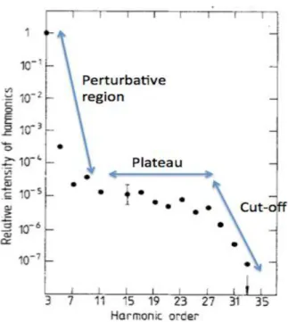
The spectrum of high order harmonics has a characteristic form, which contains three parts: the perturbative region, the plateau and the cut-off (Fig 1.10). It can be well calculated using a semi-classical model except the behavior of the cut-off region. Accurate HHG calculations are now obtained using a quantum model based on the strong field approximation (Lewenstein model) [7].
Since the HHG process is trigged by the laser’s electric field, the emitted photons are coherent, which is the basic for lens-less imaging. HHG has other advantages, such as the attosecond pulse structure, which is demonstrated in form of attosecond pulse train in 2001 [8]. We can also cite its natural synchronization with the driving infrared laser, which makes it suitable for ultrafast dynamics studies in a pump-probe geometry. I also would like to point out that the
HHG source has been used to seed a soft X-ray FEL resulting in pulse with improved temporal coherence [9].
Fig. 1.10. A typical spectrum of HHG with three parts: perturbative region, plateau and cut-off. The original spectrum is extracted from Ref 22.
Practically, in the context of the application of HHG in lens-less imaging, we usually choose the harmonics in the plateau. They are usually more intense and stable than the cut-off harmonics. We also select through phase matching the short trajectory that exhibits better spatial and spectral coherence properties than the long trajectory.
II.2Experimental set-up
All the imaging experiments in this thesis work have been accomplished using the High flux harmonic beamline at the CEA Saclay research center, France. The harmonic beamline is a
The three experimental chambers of the High flux harmonic beamline are (Fig. 2.1):
1) HHG chamber: Up to 50 mJ laser energy can be focused into a gas cell to generate harmonics beam. The gas cell is a metal tube with two pinholes at its extremes filled with rare gas. We have easy and full motorized control of the gas cell in vacuum: the cell length is variable from 0 to 15 cm and its lateral position (y direction) to the beam propagation direction (z) is motorized by a translation stage; we can also adjust the orientation of the cell in z direction by tilting it in x and y directions (perpendicular to z) with precision.
2) Optics chamber with ‚imaging configuration‛: The harmonics and IR beams propagate together into the optics chamber. An IR antireflective mirror separates them and sends the harmonics beam to the diffraction chamber. The residual IR is then filtered by aluminum filters located between the optics chamber and the diffraction chamber. 3) Optics chamber with ‚spectrum configuration‛: We can also replace the IR antireflective
mirror by a pair of toroidal mirror and plane grating for spectrum studies. The thin slit and the photomultiplier tube (PMT) are located at the end of the setup. We can also replace the PMT by an XUV camera to measure the harmonic beam profile in the far field or even an XUV wave front sensor.
4) Diffraction chamber (Fig. 2.2): The multilayer parabolic mirror (coated by Institut d’Optique) selects one harmonic order (25th harmonic in our experiments) and focuses the beam onto the sample located at its focus. The CCD camera behind the sample holder detects the diffraction pattern in the far field regime.
This harmonic beamline has delivered its first photons in 2007. First demonstration of CDI reconstructions of a test object has been published in 2009. This has encouraged further studies in lens-less imaging and beamline optimization. This chapter will follow the time line to present the ‚High Flux Harmonic‛ beamline developments.
Fig. 2.1.Scheme of the High flux harmonic beamline. The red arrow at left bottom indicates the beam propagation direction. The infrared beam is first focused into a gas cell in the harmonic generation chamber. The optics chamber separates the harmonics beam from the IR beam and sends it into the diffraction chamber where the lens-less imaging experiments will take place. The optics chamber can also switch to a TM-PGM (Toroidal Mirror-Plane Grating Monochromator) type spectrometer for HHG studies. The entire setup is about 5 meters long.
Fig. 2.2.Picture of the diffraction chamber. The parabolic mirror focuses the harmonics beam onto the sample, and the CCD camera located behind the sample holder detects the diffraction pattern.
II.3 HHG optimization and beamline standardization
I present in this section the effort to build a powerful, stable and reproducible harmonic beamline for imaging applications. The principle goal is to realize dynamical visualization (2D or 3D) of
ultrafast physical phenomena on a femtosecond scale with nanometric spatial resolution. In coherent imaging, the X-ray photon flux on sample (single shot or multiple shots) determines the signal extension on the diffraction pattern (the maximum spatial frequency of the diffracted signal). A high signal extension corresponds to a high theoretical spatial resolution (Eq. 1-29, Chapter I). Moreover, the radiation damage of samples (especially biological ones) limits the maximum pulse energy for each shot, which is a real limitation for light sources that provides high average but low peak flux beam, such as synchrotrons. However, one can achieve high-resolution imaging with another strategy. The idea is to irradiate the sample with a single pulse short enough to capture the image before the onset of the radiation damage. The FEL or XFEL facilities can provide such X-ray pulses. HHG source has demonstrated such potential however further work was necessary to improve the quality of the CDI diffraction patterns. In this thesis work I present the optimization of the entire beamline (HHG process and all the optics) to finally get the maximum pulse energy available on sample for high-resolution single-shot
imaging. It has been also important to standardize the beamline to have stable beam performances, which was at the very beginning of my work unstable from day to day.
The harmonic beamline optimization has been realized in two steps:
1) HHG optimization: As mentioned before, we would like to maximize the harmonic pulse energy to get higher reconstruction resolution. However, it is not the only factor that influences the reconstruction quality. The wave front, the coherence and the spatial distribution of the intensity of the harmonic beam are also critical factors. The HHG optimization process conducted here has been to find an optimum compromise between all these factors to enhance the quality of diffraction patterns or holograms.
2) Focusing optimization: The sample is located at the focus of the parabolic mirror. The phase retrieval algorithms reconstruct the exit wave at the object plane (Chapter I, section I.2) that is equal to the sample transmittance in case of a plane wave illumination. Thus the harmonic beam focusing quality has a large influence on the reconstruction result. We need a homogenous focal spot and a proper spot size compared to samples. We have used a Hartmann type wave front sensor to characterize and evaluate the quality of the generated harmonics beam before and after focusing optics (the parabolic mirror). The wave front sensor measures the wave front and the intensity of the harmonic beam, and reconstructs the beam profile using back-propagation functions. First we place the wave front sensor at a distance of 5 m from the gas cell without any focusing optics (Fig. 2.3). We measure the direct harmonics beam in far field and optimize the wave front as a function the HHG parameters, such as IR laser energy, IR beam aperture, gas cell length, gas pressure and etc. Then, we align the wave front sensor after the focus of the parabolic mirror to characterize and optimize the focal spot.
After the optimization process with the wave front sensor, we use a Young’s double slits to characterize the harmonic beam coherence, and study the influence of the coherence on phase retrieval reconstructions. We measure the variations of the beam coherence using a similar process as the HHG optimization with the wave front sensor. The results show that it could be an alternative way to optimize the beamline, but less efficient and less accurate than the wave front sensor, because one has to check manually the fringe visibility of each interference pattern and only a small part of the beam is characterized in each measurement.
Fig. 2.3.Scheme of the optimization experiment setup. 1) HHG optimization configuration: Movable mirror 1 (multilayer plane mirror) is in and the wave front sensor is located at position 1 to measure the direct harmonics beam. 2) Focusing optimization configuration: Movable mirror 1 is out and mirror 2 is in; the wave front sensor is located at position 2 to measure the focused harmonic beam by the parabola. 3) Diffraction configuration: Two movable mirrors are out and no wave front sensor. The sample (Young’s double slits) is located at the focus of the parabola and the XUV camera detects the diffraction pattern (far field interference of the slits exit waves).
II.3a HHG optimization and beamline standardization: wave front sensor
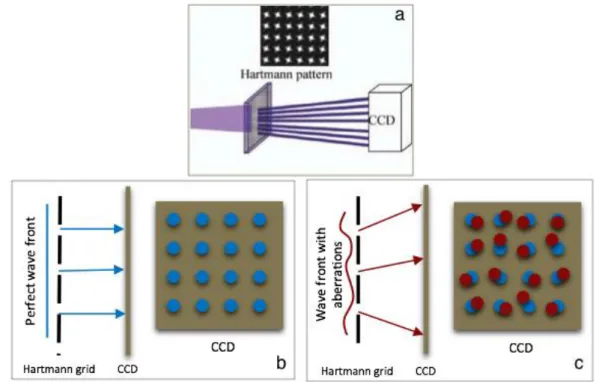
The Hartmann type wave front sensor ‚HASO‛ (produced by Imagine Optics Corp.) is composed of a Hartmann pattern grid and a XUV camera located 20 cm behind the grid (Fig. 2.4a). The harmonic beam goes through the Hartmann grid, which is an array of holes, and projects the ‚beamlets‛ sampled by each hole onto the XUV camera. The positions of the individual spot centroids are measured (Fig. 2.4c) and compared with reference positions (calibrated with perfect wave front, Fig. 2.4b). The measured local shifts of each beamlet can reconstruct the wave front of the harmonic beam. The measured beamlets present also the harmonic beam’s intensity profile at a sampling rate of the grid. One can then deduce the aberrations of the beam. Using back-propagation functions, the harmonic beam profile at the point source can be reconstructed. These numerical calculations are realized within the paraxial approximation.
The wave front sensor is calibrated and provided by the research group of P. Zeitoun at Laboratoire d'Optique Appliquée (LOA), France. The Hartmann grid is 19 x 19 mm2 large and contains 51 x 51 square holes that each is 80 x 80 μm2 large and separated by 380 μm. The back-illuminated CCD camera has 2048 x 2048 pixels of 13.5 x 13.5 μm2 each, operating at -40 °C. The typical calibration method is presented in Ref 14. In our case, a 10 μm pinhole positioned in the beam propagation path at 1 m from the gas cell output diffracts the beam and generates a
perfect wave front. The sensor accuracy is then experimentally measured to be λ/50 RMS (root mean square) at a wavelength λ = 32 nm, i.e. an accuracy of 0.64 nm RMS [10]. Note that an aberration of λ in amplitude corresponds to local phase aberration of 2π. One should be careful when using such a sensor to measure a wave front with very strong aberrations. The mismatch of beam lets and the reference positions could lead to wrong reconstruction of wave front if the aberration exceeds 2π. In our case, the harmonic beam has relatively week aberrations so that the sensor is well adapted.
Fig. 2.4.Scheme of the Hartmann type wave front sensor. (a) The target beam goes through the Hartmann pattern grid, which is an array of holes, and projects onto the XUV camera behind. The XUV camera detects the sampled intensity of the beam. (b) The wave front sensor should be calibrated with a perfect beam before first use. The positions of the beam lets on the camera will be registered as reference positions (blue points). (c) The wave front is reconstructed from the measured local shift (red points) of each beam let compared to the reference positions.
In the first step, we have explored systematically several HHG parameters to optimize the harmonic flux and the beam wave front RMS value. The wave front RMS value describes how the measured wave front is distorted compared to a plane wave. According to the Maréchal’s
beam is stable that measurements can be achieved in different shots, the relative position of the beam when hitting onto the sample should be known for extracting correctly the sample transmittance information.
In our experiment, we have optimized the wave front RMS value to the diffraction-limited (λ/14) and maximized the harmonic flux. The initial IR beam has a diameter of about 40 mm and is then limited in aperture by a diaphragm located in front of the focusing lens. We conclude the optimum parameters’ value range: beam aperture = 20~21 mm, gas pressure = 8~9 mbar, gas cell length = 5~8 cm, effective laser energy = 15 mJ and the focus position is 2 cm behind the gas cell output. The beam aperture of 20~21 mm corresponds to a laser focal radius of 137~143 μm and the confocal parameter = 14,7~16 cm. The harmonic flux and the wave front RMS share the same optimum value range and are maximized with the same parameter values, which agrees with previous work [10].
For each wave front measurement, aberration contributions are calculated with Zernike polynomials, which is unstable from shot to shot. There is no obvious relation between aberration contributions and the harmonic generating conditions. Previously, two groups working on HHG optimization with wave front sensor reports trade-off conclusions of harmonic aberrations dependence on pump laser aberrations [10]. A further study on the aberration dependence of the High flux harmonic beamline is planned and it may lead to new HHG optimization.
The harmonic beam generated with optimum parameters has a wave front RMS of 0.11λ (λ/9), compared to a non-optimized harmonic beam whose wave front RMS is 0.79λ (Fig 2.5). Meanwhile, the spatial profile of the harmonic beam in far field has also been optimized, which is important for coherent imaging. The reconstructions of the harmonic beams at the source are shown in the Fig. 1 attached article.
Fig. 2.5. Generating condition: gas pressure = 8 mbar, gas cell length = 8 cm, laser energy = 15 mJ, beam aperture = 24 mm for (a) and (b), and 21 mm for (c) and (d). (a) is the measured intensity and (b) is the measured phase of the non-optimized harmonic beam by the wave front sensor in far field. (c) and (d) are respectively the intensity and the phase of the optimized harmonic beam. Note that the absolute phase scales in (b) and (d) are different.
II.3.b HHG optimization and beamline standardization: Focusing optimization
In the second step, the wave front sensor is located behind the focus of the parabolic mirror to characterize the harmonic focal spot, which represents the illumination condition for coherent imaging. In the beam path from the harmonic source (output of the gas cell) to the sample (focus of the parabolic mirror), there are only two optics (IR-antireflective mirror and parabola) and one aluminum filter. The focusing quality, thus the illumination quality is strongly related to the alignment of the parabola. The parabola is motorized by translation stages and goniometers. It is initially aligned with residual IR beam as reference. The study with a wave front sensor allows direct measurements of the focusing quality with the harmonic beam (25th order) in the same condition as the coherent imaging. A fine adjustment is then possible for the parabola motorized in all translation and tilt directions to optimize the focal spot. Finally, the wave front sensor measurements in this configuration characterize the whole harmonic beam line until the diffraction stage by taking account of all elements in the beam line except the detection part. The optimization of the detection stage is associated to each particular imaging configuration, including sample conditions, imaging technique, final resolution, illumination quality, etc. It will be discussed in the following chapter.
Experimental results show that a fine adjustment of the parabola with the harmonic beam can optimize the focal spot’s spatial profile and aberrations. Fig 2.6 shows the enhancement of the harmonic beam before and after the fine adjustment of the parabola. We get a harmonic beam of 0.154λ (~λ/6) RMS (Fig. 2.6d) instead of 0.326λ (~λ/3) RMS (Fig. 2.6b) measured at the Hartmann grid. Usually, the dominant aberration of the harmonic beam is the coma, which should be associated to the miss-alignment of the parabola. It is clearly observed in the reconstruction of the focal spot before fine adjustment. The focal spot after fine adjustment presents a homogenous and quasi-circular beam profile, with reduced coma aberration. The beam size (at 1/e2) is optimized from 7.8 μm to 5 μm, which matches better our samples (usually within a
Fig. 2.6. (a) is the intensity and (b) is the phase of the 25th harmonic beam with initially aligned measured by wave front sensor. (c) and (d) are respectively the intensity and the phase of the harmonic beam with finely tuned parabola.
In the beam propagation direction (z direction), the focused harmonic spot changes quickly before and after the parabola focus position. The evolutions in both conditions (before and after fine adjustment) are similar, while the optimum adjustment provides quasi-circular focal spot in a range of ±0.5 mm around the focal position, larger than in the other case (Fig. 2.7). This range is important for the coherent imaging as it give flexibility in positioning the sample. Usually, we use a sharp edge (for example, the edge of the sample membrane) to look for the focus position (Fig. 2.8). Typically, we can find the focus position with a precision of ±0.2 mm, which fits the previous range of ±0.5 mm. Note that a daily alignment of the IR laser during the initiating stage of the harmonic beam line is required, which could be critical for the harmonic focusing quality. The IR laser should be aligned as it was for the fine adjustment with wave front sensor to ensure an optimum focal spot. A permanent installation of wave front sensor in focusing optimization configuration could be a precise method for daily alignment, especially for experiment projects spanning over months. According to our experience, careful daily alignment (without wave front sensor) is sufficient for short-term experiments.