Discrete-time randomized sampling

Discrete-Time Randomized Sampling

by

Maya Rida Said

B.S. Biology

B.S. Electrical Engineering and Computer Science

Massachusetts Institute of Technology, 1998

M.S. Toxicology

Massachusetts Institute of Technology, 2000

Submitted to the Department of Electrical Engineering and Computer Science

in partial fulfillment of the requirements for the degree of

Master of Engineering

at the

MASSACHUSETTS INSTITUTE OF TECHNOLOGY

February 2001

©

Massachusetts Institute of Technology 2001. All rights reserved.

Author ...

... ...

...

Department o

ngineering and Computer Science

December 22, 2000

Certified by...

Alan V. Oppenheim

Ford Professor of Electrical Engineering

Thesis Supervisor

A ccepted by ... . ... . . ... ..

Arthur C. Smith

Chairman, Department Committee on Graduate Theses

MASSACHUSETTS INSTITUTE OF TECHNOLOGY

Discrete-Time Randomized Sampling

Maya Rida Said

Submitted to the Department of Electrical Engineering and Computer Science on December 22, 2000, in partial fulfillment of the

requirements for the degree of Master of Engineering

Abstract

Techniques for developing low-complexity, robust Digital Signal Processing (DSP) algo-rithms with low-power consumption have become increasingly important. This thesis ex-plores a framework, discrete-time randomized sampling, which allows the design of algo-rithms that meet some desired complexity, robustness or power constraints. Three distinct sampling schemes are presented based on randomized sampling of the input, of the filter im-pulse response, and iterative randomized sampling of the filter imim-pulse response. Additive noise models are derived for each approach and error characteristics are analyzed for both white and colored sampling processes. It is shown that semi-white iterative randomized sampling leads to better error characteristics than white sampling through higher SNR as well as noise shaping. Discrete-time randomized sampling is then used as a filter approxima-tion method and condiapproxima-tions are derived under which a randomized sampling approximaapproxima-tion to the Wiener filter is guaranteed to lead a smaller mean-square estimation error than the best constrained LTI approximation. A low-power formulation for randomized sampling is also given and the tradeoff between power consumption and output quality is examined and quantified. Finally, this framework is used to model a class of random hardware failures and two algorithms are presented that guarantee a desired SNR level at the output under a given probability of hardware failure.

Thesis Supervisor: Alan V. Oppenheim Title: Ford Professor of Electrical Engineering

Acknowledgments

First and foremost, I would like to thank my thesis advisor, Al Oppenheim, for proving to me and convincing me that mayan just-in-time computation is inefficient since there is no processor idling time and therefore throughput is not constant. Al's mentorship and friendship have played a tremendous role in nurturing my interests in research and teaching and I am looking forward to many more years of stimulating interaction and personal growth. Al, thanks for everything, now we're ready to begin!

I am also grateful to Li Lee and Albert Chan for many hours of valuable technical discussions. My thanks go to Joe Saleh, Hur Koser, Lukasz Weber, Diego Syrowicz, and Jason Oppenheim for closely following the thesis progress.

The unconditional unlimited love of my family is a treasure that I will cherish forever. This thesis, like any other accomplishment, would have never been possible without their support. My deepest thanks also go to my great uncle, Wafic Said, for his constant support

and belief in me.

Finally, I was extremely fortunate to get to know and work with Gary Kopec the summer of 1997 at Xerox PARC. The two months I interacted with Gary had a tremendous impact on me. His focus, determination, and joie de vivre will always be engraved in my mind and I will always regret not going back to PARC the following summer. Gary, you will always

Contents

1 Introduction 15

1.1 Efficient Convolution . . . . 16

1.2 Low-Power Signal Processing . . . . 17

1.3 Hardware Failures . . . . 19

1.4 Thesis O utline . . . . 20

2 Discrete-Time Randomized Sampling 21 2.1 D efinition . . . . 21

2.2 Linear Noise Models . . . . 22

2.2.1 DTRS of the Input Signal . . . . 23

2.2.2 DTRS of the Impulse Response . . . . 24

2.2.3 Iterative DTRS of the Impulse Response . . . . 24

2.3 Error Analysis . . . . 25

2.4 Non-White Sampling . . . . 27

2.4.1 IDTRS using a Correlated Sampling Process at each Convolution Step 28 2.4.2 IDTRS using a Sampling Process Correlated across Output Samples 29 2.5 Sum m ary . . . . 30

3 Filter Approximation Based on Randomized Sampling 31 3.1 Approximate Filtering Formulation . . . . 32

3.2 Linear Minimum Mean-Square Estimation with Complexity Constraints . . 33

3.2.1 Mean-Square Estimation Error . . . . 34

3.2.2 Zero-Mean, Unit-Variance, White Process, r[n] . . . . 36

3.2.3 Non-White r[n] . . . . 38

4 Low-Power Digital Filtering

4.1 Low-Power Formulation . . . .

4.1.1 Switching Activity Reduction . . .

4.1.2 Supply Voltage Reduction ...

4.1.3 Total Power Savings ...

4.2 Tradeoff between Power and Quality . . .

4.3 Summary . . . .

5 Hardware Failure Modeling

5.1 Hardware Failure Model ...

5.2 Bandlimited Input . . . . 5.3 Parallel Filters . . . . 5.4 Summary . . . . 6 Conclusion 6.1 Thesis Contributions . . . . 6.2 Future Directions . . . .

A Derivations for White Sampling A.1 mry[n] and e1[n] are uncorrelated ...

A.2 The autocorrelation of the error: Reie, [m] A.3 mry[n] and e2[n] uncorrelated ...

A.4

A.5 mry[n] and e3[n] are uncorrelated . . . . .

A.6 The Autocorrelation of e3[n]: Ree 3[m] . .

B Derivations for Non-White Sampling

B.1 Ree₃ [iM] _{in the case of correlated sampling at each convolution step} . . .

B.2 Ree 3[IM] in the case of a sampling process correlated across output samples

39 . . . . 39 . . . . 40 . . . . 4 1 . . . . 44 . . . . 45 . . . . 46 49 . . . . 49 . . . . 5 0 . . . . 5 5 . . . . 5 7 59 59 61 63 . . . . 6 3 . . . . 6 5 . . . . 6 5 . . . . 66 . . . . 67 . . . . 68 69 69 70

List of Figures

2-1 Linear Model for Discrete-Time Randomized Sampling of the Input. .... 23

2-2 Linear Model for Discrete-Time Randomized Sampling of the Impulse

Re-sponse... ... 24

2-3 Linear Model for Iterative Discrete-Time Randomized Sampling of the

Im-pulse Response. . . . . 25

3-1 Block Diagram of the LTI Approximation of h[n]. . . . . 32

3-2 Re-Scaled IDTRS. h, [n; k] is the sampled version of h[n] as explained in

Chapter 2 and mr is the mean of the sampling process. . . . . 33

3-3 Boundary Condition for the LMMSE Approximation Problem. IDTRS

Out-performs any LTI Approximation Technique if -k-. e. > 37

any~E Zh2. [k] 2mr-1...

4-1 Original System . . . . . 40

4-2 FIR Filter Structure for Low-Power Filtering Using Discrete-Time

Random-ized Sampling. MUX is used as an abstraction to a collection of multiplexers. 41

4-3 FIR Filter Structure for Low-Power Filtering using Randomized Sampling. 42

4-4 Relative percent power consumption as a function of the sampling process

mean mr. A value of a = 1.3 was used in this simulation. [Chandrakasan et

al. [6] derive a similar relationship where the relative power consumption is

plotted as a function of the normalized workload.] . . . . 43

4-5 Normalized propagation delay and average switching power dissipation for

three values of a. The value a = 1.3 correspond to the value for 0.25-pm technology [9] while the other two values are the upper and lower bound for a. 45

4-6 Relative percent power consumption as a function of the gain in SNR at the

5-1 Direct Form Implementation of an FIR Filter. . . . . 50

5-2 Transposed Direct Form Implementation of an FIR Filter. . . . . 50

5-3 FIR Filtering using a Faulty FIR Filter with Output Scaling. . . . . 51

5-4 Additive Noise Model for the Faulty FIR Filter with Proper Re-scaling Shown in Figure 5-3. e[n] is a zero-mean wide-sense-stationary white noise with

variance 1-mRxx[0]Rhh[0]. . . . . 51

5-5 The Value of N Needed to Maintain a Given Gain in SNR. The probability

of a hardware failure is given by (1 - m,). . . . . 52

5-6 Gain in SNR as a Function of m, for Different Values of N. The probability

of a hardware failure is given by (1 - m,). . . . . 52

5-7 Gain in SNR as a function of N for different values of mr. . . . . 53

5-8 Original System with Scaling. . . . . 53

5-9 Derivation of hp[n]. LPF is a low-pass filter with cutoff - and gain N. . 54

5-10 Up-sampled Realization of Figure 5-8. LPF1 is a low-pass filter with cutoff V and gain N while LPF2 is a low-pass filter with cutoff -E- and unit gain.

It is assumed that only h.,[n] is implemented on the faulty hardware. . . 54

5-11 Sensor Network. . . . . 55 5-12 Sensor Network Model . . . . . 56

List of Tables

1.1 Individual power components contributing to the overall time-averaged power

consum ption. . . . . 18

2.1 Autocorrelation Functions of the Errors obtained from each Sampling Scheme

using a White Sampling Process. . . . . 26

2.2 In-band Signal-to-Noise Ratios for the Three Sampling Methods. . . . . 26

Chapter 1

Introduction

Signal processing algorithms are designed to satisfy a variety of constraints depending on the application and the resources available. For example, when the amount of computation or the processing time is an issue, algorithms should be optimized for computational or time efficiency. Low-power algorithms, on the other hand, are used in environments where power is limited such as battery-powered mobile devices. Other situations present the need for robust algorithms in order to maintain a given performance level during hardware failure. Recently, with the rising demand for small mobile devices, there has been an increasing need for efficient, reliable, and low-power signal processing algorithms. In this thesis, we define a framework, discrete-time randomized sampling, with potential applications in the areas of hardware failure modeling, efficient algorithm development, and low-power signal processing. By randomly sampling signals or filters, this approach allows the modification

of pre-existing algorithms to meet certain complexity, robustness or power constraints. Randomized sampling is defined within the broader randomized signal processing frame-work used when the signal conversion or processing procedures are performed stochastically. Randomized signal processing is therefore fundamentally different from statistical signal processing where randomness is only used as a representation of signals. When sampling is performed at random time-intervals, it is described as randomized. Most of the randomized sampling literature starts from a continuous-time signal and thus consists of a randomization of the sampling process. Bilinskis and Mikelsons [2] survey the current results and issues in this area. By dealing with randomness exclusively in discrete-time, the framework presented by this thesis is distinct from the common approach found in the literature. Discrete-time

randomized sampling could therefore be thought of as randomized down-sampling.

The approach developed in this thesis leads directly to three major applications in the areas of efficient convolution, low-power signal processing and hardware failures. In the remainder of this chapter, we present some relevant background in each of these areas. We then conclude with an outline of the thesis.

1.1

Efficient Convolution

Linear time-invariant (LTI) systems are widely used in signal processing applications, mainly because they can be analyzed in great detail and present good models of many physical phe-nomenon. A major advantage of discrete-time LTI systems is their ability to be fully char-acterized by the convolution sum. Implementing a filter is thus equivalent to implementing a convolution, and since processing power is usually an issue, efficient implementations tend to be favored. In general, convolution can be implemented either in the time or frequency domains. The fast Fourier transform (FFT) algorithm made the frequency-domain imple-mentation of convolution much more computationally attractive since the impleimple-mentation of a length N convolution using block processing and fast Fourier transforms requires an order of NlogN multiplications per block of input, while the same operation implemented

directly in time requires N 2 multiplications. However, frequency-domain processing leads

to delays of the order of the filter length which is undesirable in some practical applications such as echo cancellation. In fact, many current Digital Signal Processing (DSP) chips implement convolution in time which can result in a very large computational complexity in applications where the filters have several thousands of coefficients. There have been sev-eral approaches to deal with this increased complexity. One class of approaches generates algorithms with exact solutions, i.e. no errors are introduced. Examples of such approaches include the parallel-decomposition algorithm of Wang and Siy [20] and the non-uniform partitioned block frequency-domain adaptive filter of Egelmeers and Sommen [7]. While these methods can be attractive because they do not introduce any distortions, they often either require specialized hardware or involve complex filter manipulations.

Simpler efficient algorithms can usually be obtained, at the cost of errors, from filter approximation techniques which reduce the filter length, and therefore reduce the amount of multiplications and additions in the convolution. Two common approximation techniques

are the window method and the Parks-McClellan algorithm. While both tend to be used to obtain FIR filters from IIR filters, these procedures can also be used to approximate long FIR filters with shorter ones. By truncating the original filter, the rectangular window method provides the best mean-square approximation to a desired frequency response for a given filter length, i.e. it minimizes E, h! [n] where he [n] is the error filter which is defined as the difference between the original filter and the truncated filter. The Parks-McClellan algorithm, on the other hand, minimizes the maximum magnitude of the error filter, i.e. it minimizes Max(IHe(ejw)I).

In this thesis, we present randomized sampling as an alternative filter approximation technique and, therefore, a method for efficient computation. In fact, by randomly setting some of the filter coefficients to zero, randomized sampling can be used as a procedure to perform only a subset of the multiplications in the convolution sum. An investigation of this technique will be carried out in Chapter 3.

1.2

Low-Power Signal Processing

Another area of interest in signal processing, power consumption, gained more attention in the early 90's due to the advances in storage and display technologies. These advances significantly reduced the power consumption due to the transfer of data and, as a result, increased the proportional power consumption by the processing modules [14]. A current major concern when developing signal processing algorithms for portable devices is to

min-imize the total power consumption in order to maxmin-imize the run-time while minimizing battery size [5]. In general, power can be minimized at four different levels: technology, cir-cuit approaches, architectures and algorithms. Various techniques have been developed to reduce power consumption in digital circuits and research in this area is gaining tremendous attention. Brodersen et al. [3], present a good discussion of the relative gain to be expected from each of these areas while Evans and Liu [8] survey several low-power implementation strategies for common processing modules.

While both peak and time-averaged power are important factors in low-power systems design, battery size and weight are only affected by the average power. The time-averaged power consumption in CMOS digital circuits can be divided into four different components

due to short-circuit, leakage, static, and switching as shown in equation 1.1 [13].

Paverage = _{Pshort-circuit + 'leakage + Pstatic + Pswitching}

(1.1)

All four components are affected by the supply voltage, Vdd. In addition, the first three components depend on the short-circuit, leakage, and static currents respectively while the last component depends on the load capacitor, CL, the operating or switching frequency,

fs,

of a power consuming transition. Table 1.1 gives mathematical expressions for all four components.

Table 1.1: Individual power components consumption.

contributing to the overall time-averaged power

In general, the switching power component is responsible for more than 90% of the total average power consumption [3]. As a result, switching power has gained great attention in low-power design. In general, algorithm design has little or no effect on power consumption resulting from leakage, short-circuit, or static, but it can play a major role in reducing the power due to switching. To first order, the average switching power consumption of a signal processing task can be written as:

(1.2)

Pswitching

where Ci is the average capacitance switched per operation of type i corresponding to

ad-Short-circuit power Pshort-circuit = 'short-circuit Vdd

Static power Pstatic = IstaticVdd

Leakage power 'leakage = IleakageVdd

dition, multiplication, storage, or bus access. Ni is the number of operations of type i

performed per output sample. Vdd is the operating supply voltage while

f,

switch-ing frequency. Traditionally, the switchswitch-ing frequency is fixed in many signal processswitch-ing applications [6] and Ci is adjusted at the physical or circuit level. As a result, algorithm optimization for low-power processing has been mainly concerned with minimizing Ni. Sev-eral filter approximation methods have been used to explore low-power algorithms. Ludwig

et al. [12], for example, use approximate processing to adaptively reduce the number of

operations switched per sample based on signal statistics. They propose an adaptive fil-tering technique applied to frequency selective filters which dynamically chooses the lowest filter order that is guaranteed to achieve a preset output SNR. Pan [18], on the other hand, reduces power dissipation using approximate processing by taking advantage of the nature of audio signals. He uses adaptive filtering algorithms to reduce power by dynamically minimizing digital filter order. Chapter 4 of this thesis presents an algorithmic approach to low-power based on randomized sampling. Considerable power savings are obtained by

reducing Ni, Vdd, and

f,

1.3

Hardware Failures

With the increase in dependability on digital systems, robustness is yet another issue to address when designing signal processing algorithms. Even with the use of high quality components and design techniques, there is always a non-negligible probability of system failure: robust algorithms should therefore be designed to deal with such failures. Most of the work in this area has been in the development of fault tolerant systems which are achieved through redundancy in hardware, software, information and/or computation [17]. Jiang et al. [10], for example, use adaptive fault tolerance for FIR filters to compensate for coefficient failures in an FIR adaptive filter by adding extra coefficients. Because of cost constraints, most of the fault tolerance strategies tend to address only single, statistically independent faults. However, multiple faults are very common especially with complex in-tegrated systems and thus are receiving increased attention. Another disadvantage of the fault tolerance strategy is that it usually leads to very complex and inefficient algorithms. This can be particularly undesirable if only an acceptable, and not necessarily exact, perfor-mance is needed. An alternative approach to fault tolerance briefly explored by this thesis

is the design of robust algorithms that are guaranteed to maintain a given signal-to-noise ratio in the presence of some types of hardware failures. This approach, while it does not guarantee a fault-free system, is generally much simpler and can be implemented efficiently. Chapter 5 lays out the hardware failure model and presents techniques for maintaining a desired level of performance under some types of hardware failures.

1.4

Thesis Outline

The thesis is organized as follows: in Chapter 2 we define the discrete-time randomized sampling framework by presenting three distinct sampling algorithms. Error models and properties are also derived for each sampling procedure. Discrete-time randomized sampling is then presented in an approximate filtering context in Chapter 3. Performance measures are defined and the randomized sampling algorithms are compared to LTI approximate pro-cessing techniques such as the rectangular window method. A low-power digital filtering formulation for discrete-time randomized sampling is given in Chapter 4. Power savings are evaluated and the trade-off between power and system performance is analyzed. Chapter 5 defines hardware failure models where the algorithms described in Chapter 2 are representa-tive of the distortion introduced by the faulty system. As a result, techniques are derived to guarantee a desired performance level under a given probability of failure. Finally, Chapter 6 concludes by summarizing the contributions of the thesis and further research directions are suggested.

Chapter 2

Discrete-Time Randomized

Sampling

In this chapter, we define discrete-time randomized sampling and present three different sampling approaches in the context of LTI filtering. We then derive linear noise models for each case and give second-order characteristics for the errors resulting from both white and colored sampling processes. Further error analysis is then presented by examining the in-band SNR obtained from each approach.

2.1

Definition

Discrete-time randomized sampling (DTRS) refers to any process which randomly sets some of the sample points of a discrete-time signal or filter impulse response to zero. DTRS is defined in the context of a general LTI system where the impulse response, h[n], is deterministic and the input and output signals, x[n] and y[n], are wide-sense-stationary stochastic processes. The sampling can essentially be applied to the input, x[n], or the filter, h[n].

Sampling the input consists of randomly setting some of the input signal samples to zero. This can be viewed as a randomized down-sampling procedure where the randomization is at the signal conversion level. It is modeled as a multiplication by a non-zero-mean

1. The resulting output, ysi[n], can then be written as:

+00

Ysi[n]

= (x[n]r,[n]) *

h[n]

=

E

x[k]rs[k]h[n

-

k]

(2.1)

k=-oo

In the remainder of this thesis, this procedure will be referred to as DTRS of the input. DTRS can also be applied to the filter impulse response. Sampling the filter can be performed in two ways. First, a one-pass sampling scheme can be applied in which the filter is sampled only once and then the resulting filter is used to process the signal, x[n]. We refer to this sampling scheme as DTRS of the impulse response. It consists of randomly setting some of the filter coefficients to zero which makes the processing procedure stochastic. Again, the sampling process, r,[n], is a non-zero-mean wide-sense-stationary random signal and independent of x[n]. The output, ys2[n], can then be written as:

+00

Ys2[n] = (h[n]rs[n]) * x[n] = 1 h[k]r,[k]x[n - k]. (2.2)

k=-oo

A more elaborate sampling procedure for the impulse response consists of randomly sampling the filter at each iteration of the convolution sum. We refer to this sampling scheme as iterative DTRS of the impulse response, or simply IDTRS. The resulting filter is time-varying and stochastic, and can be modeled as multiplying the impulse response by a two-dimensional random signal in which one dimension corresponds to time and the second

dimension is the ensemble member. The sampling process, r,

[n;

non-zero-mean wide-sense-stationary random signal and independent of x[n]. The output,

yS3[n], can then be written as:

ys₃[n] = x[nl]*(rs[n;k]h[n]) (2.3)

+00

- r[n; k]h[k]x[n - k]. (2.4)

k=-oo

2.2

Linear Noise Models

For each sampling method and for the case where the sampling is performed using wide-sense-stationary sampling sequences, one can derive linear noise models for the resulting distortion by rewriting the sampling process, rs[n], as the mean, mr, added to a

zero-mean process, ir[n]. Similarly the two-dimensional process, r,[n; k], can be rewritten as a dimensional zero-mean random process, r,[n; k], added to the mean, mr, where the

two-dimensional mean is defined as E(r,[n; k]) = mr. As a result, each of the above sampling

procedures can be rewritten as a scaled output added to noise. In order to gain some understanding as to the nature of the distortion introduced, second-order characterizations of the noise processes for each procedure are derived below.

2.2.1 DTRS of the Input Signal

Rewriting r,[n] as the sum of i,[n] and mr, equation (2.1) can be expressed as a scaled

output added to a noise term:

Y,1[n] = h[n] * ((is[n] + mr)x[n]) (2.5)

= mr y[n] + el[n] (2.6)

where it can be shown that mry[n] and e [n] are uncorrelated (Appendix A). Furthermore,

assuming i s [n] is white, then it can be shown that:

Reiei [n] = mr (1 - mr)Rx[0]Rhh[n] (2.7)

where Rele, [n] and Rx [n] denote the autocorrelation functions of the error and the input

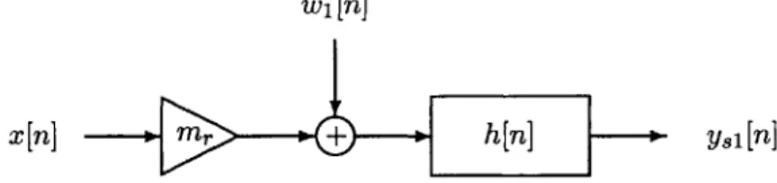
signals respectively, and Rhh[n] is the deterministic autocorrelation of the impulse response. This method can thus be modeled as adding white noise to the scaled input signal and then filtering the resulting signal with h[n] as shown in Figure 2-1. wi[n] is a zero-mean

wide-sense-stationary white noise process with variance mr (1 - mr)Rxx [0].

w,[n]

x[n] 'Mr + h[n] y.1[n]

2.2.2

DTRS of the Impulse Response

Following the same approach as in the previous section, Ys2[n] can be expressed as a scaled

output added to a noise term:

Ys2[n] = x[n]*(( s[n]+mr)h[n]) (2.8)

= mry[n]+ e2[n]. (2.9)

Again, it can be shown that mry[n] and e2[n] are uncorrelated. In addition, assuming ,[n]

is white, then the autocorrelation of the error, Re2e2[n], is given by:

Re2e2[n] = mr (1 - mr)Rxx[n]Rhh[0]. (2.10)

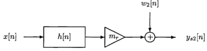
This method can thus be represented as adding colored noise to the scaled output, as shown

in Figure 2-2. The noise spectrum has the same shape as the input power spectrum: w2[n]

W2 [n]

x[n] h[n] Mr + ys2[n]

Figure 2-2: Linear Model for Discrete-Time Randomized Sampling of the Impulse Response.

is a zero-mean colored noise with autocorrelation mr(1 - mr)Rhh[O]Rxx[n].

2.2.3 Iterative DTRS of the Impulse Response

We can rewrite Ys3[n] as :

ys3[n] = x[n]* ((Ps[n;k]+ mr)h[n]) (2.11)

= mr y[n] + e3[n]. (2.12)

Again mry[n] and e3[n] are uncorrelated. In addition, we assume that i ,[n; k] is

two-dimensional white, so that the autocorrelation RA, [n; k] of P,[n; k] is given by:

and that x[n] is a wide-sense-stationary random process. Then the autocorrelation of e3[n],

Re3e3[n], is given by:

Re3e3[n] = mr(1 - mr)Rx[0]Rhh[0]J[n]. (2.14)

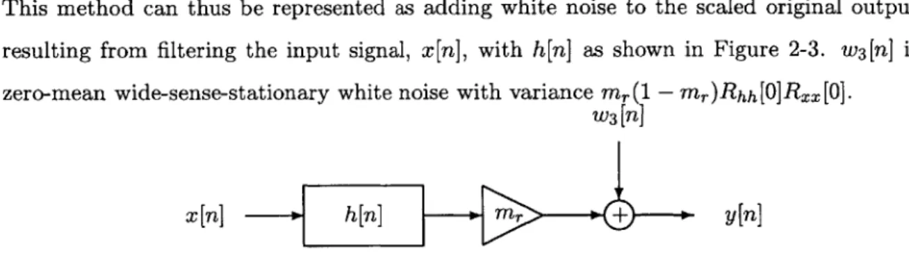
This method can thus be represented as adding white noise to the scaled original output

resulting from filtering the input signal, x[n], with h[n] as shown in Figure 2-3. w3[n] is

zero-mean wide-sense-stationary white noise with variance m, (1 - mr)Rhh[0]Rxx[0].

W3 [n]

x[n] N h[n] Mr + y[n]

Figure 2-3: Linear Model for Iterative Discrete-Time Randomized Sampling of the Impulse Response.

2.3

Error Analysis

The previous section showed that if the sampling process is wide-sense-stationary, the output from each of the three sampling procedures could be rewritten as the original output scaled by the mean of the sampling process added to an error term which was shown to be wide-sense-stationary and uncorrelated with the signal. Table 2.1 summarizes the second-order characteristics of the errors obtained when the sampling process is white. All three errors have the same total power or variance since

Reiei [0] = Re2e2[0] = Re3e3[0] = mr(1 - mr)Rx[0]Rhh[0]. (2.15)

However, they each have different spectral densities.

The signal-to-noise ratio (SNR), defined as the ratio of signal variance (power) to noise variance, is commonly used as a measure for the amount of degradation of a signal by additive noise [1]. A mathematical expression for the SNR is given in equation (2.16). It is clear that, since all errors have the same total power, the three sampling methods are equivalent if the only criteria is to maximize SNR. However, using the SNR as defined in equation (2.16) is sometimes misleading since a more relevant measure is typically the noise

Method Error Autocorrelation Function

DTRS of x[n] el[n] Reieil[n] = mr(1 - mr)Rx[O]Rhh[n]

DTRS of h[n] e2[n] Re2e2[n] = mr(1 - mr)Rhh[0]Rxx[n]

Iterative DTRS of h[n] e3[n] Ree3[n] = mr(1 - mr)Rxx [0]R hhO]S[

Table 2.1: Autocorrelation Functions of

using a White Sampling Process.

the Errors obtained from each Sampling Scheme

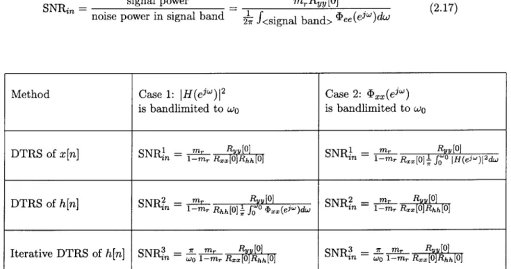
power in relation to the signal spectrum. Therefore, a more useful measure for the amount of distortion is the in-band SNR defined as the ratio of the power in the output signal to the noise power within the signal band. Equation (2.17) gives a mathematical expression for this measure and Table 2.2 lists the in-band signal-to-noise ratios for the cases when

IH(ejw)1 2 is bandlimited and when <Dxx(ew) is bandlimited.

si nanl oweUrP

SNR - variance of signal _ m[ R []

variance of noise Ree [0]

m

R

[0]

SNRin - b " 1 r yy

noise power in signal band 2 f<signal band> (Iee(ejw)dw

(2.16)

(2.17)

Method Case 1:

IH(elw)1

(Ixx(e")

is bandlimited to wo is bandlimited to wo

DTRS of

x[n]

[01

m 1-mr Rxx[OJRhhO z -0 1-mr Rx [0]-L fWO I H(eiw) 1I2

DTRS of h[n]

SNRf,

SNR?

1-M Rh [1 - f4 (xx(ew)ciW inf- 1-mr Rx]Rhh [0

Iterative DTRS of h[n] SNR- - NII1Yh

SNR=-

wb i-: I n Rhhn [5--n WO i-mr Rxx[sTRhh[hg

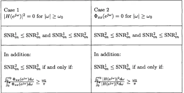
It is clear from Table 2.2 that, since ' > 1, IDTRS always leads to a higher in-band signal-to-noise ratio than DTRS of the input if the filter is bandlimited. If, on the other hand, the input has a bandlimited power spectrum, then IDTRS always leads to a higher in-band signal-to-noise ratio than DTRS of the impulse response. In addition, it follows in a relatively straight-forward way that in the case where the filter is bandlimited to wO, if the ratio of input power within the filter band to the total power in the input is greater

than ", then IDTRS always leads to a higher in-band SNR than DTRS of the filter, and

thus in this case, IDTRS leads to the highest in-band SNR. In the case where the input

power is bandlimited to wo, then it can be shown that IDTRS leads to a higher in-band

signal-to-noise ratio than DTRS of the input if and only if the ratio of power in the filter within the input band to the total power in the filter is higher than f, and in this case, IDTRS leads to the highest in-band SNR. Table 2.3 summarizes these results.

Casel Case2

IH(ejw)12

= 0 for jwI wo <Ix(eiw) = 0 for jwI wo

SNR_ < SNR3 and SNR_ < SNRf, SNRn: <SNR3, and SNR? < SNRI

In addition: In addition:

SNR_ < SNR if and only if: SNRW_, <SNRj3 if and only if:

&"<10

fow <Dxx(ej-)dw - fo IH(eiw)12dw - 7

Table 2.3: In-band SNR Comparisons for the Three Sampling Methods.

2.4

Non-White Sampling

While in previous sections, we assumed the sampling process was white, in this section, we relax this condition and explore non-white sampling in the context of iterative randomized sampling of the impulse response. In particular, having a correlated sampling process could potentially lead to better error characteristics through lower error variance or higher

in-band signal-to-noise ratio. In the following, we examine cases where the two-dimensional

sampling process, ?,[n; k], is white in one dimension and colored in the other. Specifically,

we first investigate the case where ?s [n; k] is white in the n-dimension and arbitrary in the k-dimension, we then proceed to the case where r^ [n; k] is colored in the n-dimension and white in the k-dimension.

2.4.1 IDTRS using a Correlated Sampling Process at each Convolution Step

Consider the case where the processes used to sample the impulse response in order to compute successive output samples are uncorrelated with each other. However, the process used to compute each output sample has some correlation, i.e. is not white. Then, assuming the mean of the process is mr, the autocorrelation function of the sampling process can be written as:

Rff, [m; k] = (1 - mr)mr[m]Rg[k] (2.18)

where Rgg[k] is a one-dimensional arbitrary autocorrelation function which describes the second-order statistics of i, [n; k] in the k-dimension. We can then show (Appendix B) that the autocorrelation of the error, e3[n], can be written as:

+00 +00

Rese3 [M] = Mr(1 - Mr) E E h[k]h[l]Rgg[l - k]Rxx[l - k]6[m] (2.19)

k=-oo 1=-oo

i.e. the error resulting from such sampling is still white however the variance is now different from the sampling using a two-dimensional white process. In order to gain some intuition,

consider the special case where Rgg[m] = J[m] - ao6[m - 1] - a6[m

+

i.e. where there is correlation at only one lag. In this case, equation (2.19) becomes:

Re3e3 [IM] = Mr(1 - mr)(Rhh[O]Rx[O] - 2aRhh[1]Rxx[1])6[m]. (2.20)

The variance is no longer only a function of the energy in the filter and the input, as was the case for white sampling, it now also depends on the energy at one lag in the filter and the

input. In particular, if Rhh[1] and Rxx[1] have the same sign and a is positive, or if Rhh[1]

than the one resulting from randomized sampling using a two-dimensional white sequence. This therefore suggests a method for adjusting the correlation of the sampling process in order to reduce the error variance if some information about the signal and filter is known.

2.4.2 IDTRS using a Sampling Process Correlated across Output Sam-ples

Now consider the case where at each convolution step, the sampling process is white, how-ever the processes used in computing different output time samples have some non-zero correlation. Then, if the process mean is mr, the two-dimensional autocorrelation function of the sampling process can be written as:

Rf, [m; k] = mr (1 - m,)R,,[m]6[k] (2.21)

where R,, [m] is a one-dimensional arbitrary autocorrelation function which describes the second-order statistics of i, [n; k] in the n-dimension. We can then show (Appendix B) that

the autocorrelation of the error e3 [n], can be written as:

Re3e3 [m] = Mr (1 - mr)Rhh [0] R,, [m] Rx[m]. (2.22)

The error, in this case, is no longer white and the correlation is determined by the amount of correlation in the sampling process as well as in the input. Note that in the limiting case

where R,, [m] is 1 for all m, Re3e3 [iM] = Re 2 [M], i.e. the autocorrelation function equals

the autocorrelation function resulting from DTRS of the impulse response. This should not be surprising since in the limiting case, both sampling procedures are equivalent up to second-order statistics, and as a result, the errors should have the same autocorrelation

functions. Furthermore, consider the case where R,,[m] = 6[m] - aJ[m - 1] - a6[m + 1]

where again -1 < a < 1, then equation (2.22) can be rewritten as:

Rx[] Rxx[]

Re3e3 [m] = mr(1 - mi)Rhh[O]Rxx[O](J[m] -

xx

Rxx[0] Rxx[0]

If Rxx [1] and a have the same sign, then the error power is highest at high frequencies

whereas if Rxx [1] and a have opposite signs, then the error power is highest at low frequen-cies. In fact, equation (2.23) shows that the error exhibit spectral shaping reminiscent of

the error behavior in a sigma-delta Analog-to-Digital converter. As a result, this method can be used to shape the error and increase in-band SNR.

2.5

Summary

This chapter defined discrete-time randomized sampling as a method of setting some of the samples of a discrete-time signal or filter to zero. Three methods for performing the randomized sampling were examined and linear noise models were derived for the case when the sampling process was white. Further error analysis in the case of white sampling was then presented and conditions were derived where iterative DTRS of the impulse response always outperformed the other sampling methods. Finally, two cases of non-white sampling were investigated and the resulting errors were analyzed. The observed lower error variance and noise shaping suggested trading off structure in the sampling process for improved error characteristics.

Chapter 3

Filter Approximation Based on

Randomized Sampling

Approximate Signal Processing was first defined by Nawab et al. [16] as a formal approach of trading-off quality for resources. In this Chapter, we consider the use of randomized sampling for filter approximation and therefore for trading-off quality for computation.

In various signal processing applications, one is interested in reducing the total amount of computation required to perform a filtering operation. Such applications include reduc-ing the amount of computation in order to speed up the processreduc-ing time or reduce power consumption. Approximation techniques have been used as ways to reduce computation since these techniques reduce the filter length, and therefore reduce the amount of multipli-cations and additions in the convolution. A common LTI approximation technique consists of reducing the filter length using one of the optimal FIR filter design methods such as the window method or the Parks-McClellan algorithm. All LTI approximation techniques introduce an error that can be modeled as in Figure 3-1. In this figure, h[n] represents the original desired filter of length P and he[n] the error filter resulting from approximating

h[n] with a filter of length M where M < P. Discrete-time randomized sampling of the

impulse response, as defined in the previous chapter, can be used as a filter approximation technique and a method for efficient computation since by randomly setting some of the filter coefficients to zero, randomized sampling can be used as a procedure to perform only a subset of the multiplications in the convolution sum if one checks for multiply-by-zero operations. This chapter investigates the potential of DTRS as a filter approximation

tech-x 0 h[n] - [n] ± Yapp [n]

h.[n] -- e[n]

Figure 3-1: Block Diagram of the LTI Approximation of h[n].

nique by comparing the error introduced through DTRS with errors introduced through LTI filter approximation techniques such as the rectangular window method. Error measures and specific classes of inputs are defined and explored.

3.1

Approximate Filtering Formulation

In Chapter 2, we noted that both non-iterative and iterative randomized sampling of the impulse response lead to errors with equal variances. As a result, if the performance measure is chosen to be the output error variance, we will only analyze the IDTRS case since the non-iterative case is equivalent. In addition, in Section 2.3, we showed that if the filter is bandlimited to wo and the ratio of the input signal energy within the pass-band to the total input signal energy is greater than or equal to y, iterative sampling always outperforms non-iterative sampling if the in-band SNR is the performance measure. As a result, in the following, we will assume that these conditions are met and will only focus on iterative sampling of the impulse response. In addition, we will assume that the sampling is performed using a two-dimensional wide-sense-stationary white process.

Since IDTRS in this case results in the original output scaled down by the mean of the sampling process added to white noise, we first need to re-scale the output by 1/mr in order to formulate the problem in the context of Figure 3-1. The rescaling is shown in Figure 3-2, and results in an additive noise model where the error variance is now scaled by 1/m , i.e. we can rewrite ys [n] as:

Ys[n] = y[n]+e[n] (3.1)

x[n]

h, [n; k]

1/r

ys[n]

Figure 3-2: Re-Scaled IDTRS. h,[n; k] is the sampled version of h[n] as explained in Chapter 2 and m, is the mean of the sampling process.

given by:

Ree [n] = Rxx [0] R)[0][] [n]. (3.2)

mr

Figure 3-2 and equations (3.1) and (3.2) summarize the approximate filtering formu-lation of discrete-time randomized sampling. These results can now be used to compare randomized sampling to other approximation techniques in the context of LTI filtering. An example of approximate filtering is given in the next section where the randomized sampling approach is compared to other approximation approaches.

3.2

Linear Minimum Mean-Square Estimation with

Com-plexity Constraints

In many cases, a filter is obtained by minimizing the mean-square difference between the output of the filter, #[n], and some desired signal, y[n]. Such applications include detection, prediction, and estimation. In this section we consider the problem of approximating the linear minimum mean-square estimator in order to reduce complexity where complexity is given by the amount of computation needed to obtain the estimate. The problem can be formulated as follows: we wish to obtain an approximation to the best linear mean-square estimator of the signal y[n] based on some received data, r[n]. The best linear estimator, in the mean-square sense, is the Wiener filter. If 9[n] denotes the output of the Wiener filter,

then, by definition, the mean-square estimation error, E((9[n] - y[n])2), is minimized, and

as a result, the estimation error, (9[n] - y[n]), is orthogonal to any linear function of the

data, i.e. E(A{r[n]}(y[n] - y[n])) = 0, for any linear operator A{}. In the following, we

consider two different approximation techniques to the Wiener filter. The first uses IDTRS as the approximation method while the second uses an LTI approximation technique with

distortion modeled by Figure 3-1. We wish to define conditions under which the IDTRS approximation leads to a smaller increase in estimation error than the LTI approximation.

Specifically, if E 2 designates the mean-square estimation error resulting from the IDTRS

approximation method, and et, is the mean-square estimation error resulting from the LTI approximation method, we would like to derive conditions such as equation (3.3) below

holds.

2 2 (3

ers < C: (3.3)

In the following, we will refer to the difference between the output of the original Wiener filter and the output of the approximated filter as the approximation error whereas the

estimation error refers to the difference between the desired signal and the output of the

estimator.

3.2.1 Mean-Square Estimation Error

In this section we derive expressions for the mean-square estimation error for each approx-imation technique. In general, all approxapprox-imation techniques can be represented through an additive error model where the output to the approximated Wiener filter is [n] + e[n] where e[n] is white and uncorrelated with j[n] for the IDTRS method, while e[n] is colored and correlated with [n] for the LTI method. The mean-square estimation error is therefore given by:

E2 = E(( [n] + e[n] - y[n])2) (3.4)

= E(([n] - y[n])2_{) + E(e}2_{[n]) + E(e[n]( [n]}

-y[n])) (3.5)

= E2 iener + a-2 + E(e[n]Q[n] - y[n])) (3.6) (3.7)

where ewiener is the minimum mean-square estimation error resulting from the Wiener filter and o-, is the approximation error variance (note all signals are zero-mean). As a result,

the increase in the mean-square estimation error, AE2 is given by:

In Chapter 2, we showed that the approximation error resulting from randomized sampling is uncorrelated with the output signal, i.e.:

E(ers[n] [n]) = 0. (3.9) It also directly follows that, since the randomizing process is independent of all other signals,

ers[n] is also uncorrelated with y[n]:

E(ers[n]y[n]) = 0. (3.10)

The increase in mean-square estimation error for IDTRS is therefore simply the approxi-mation error variance:

A2 _{ers rs*}= 2 (3.11)

In the LTI approximation case, the approximation error can be expressed as the convolution of the input to the filter (the data) with an error filter as shown in Figure 3-1. As a result, the approximation error is a linear combination of the input data and thus, using the orthogonality property of the minimum mean-square estimation error, we conclude:

E(ew[n]( [n] - y[n])) = 0. (3.12)

The increase in mean-square estimation error resulting from LTI approximation techniques is therefore equal to the variance of the LTI approximation error:

AE2 = - . (3.13)

Equation (3.3) is therefore equivalent to equation (3.14) below:

Ors = E(e2s[n]) < ar, = E(ew[n]). (3.14)

Expressions for or and o2s are given in equations (3.15) and (3.16) respectively where

Rrr[m] is the autocorrelation function of r[n] and Srr(e"') its Fourier transform. he[n] is

= R2rr[k]Rhehe[k] = 1i Srr(e)jHe(ed)12 (3.15) k

Or

Rrr [0]

27r

Rrrf[0]

(3.16)

mr 2xmr

-3.2.2

Zero-Mean, Unit-Variance, White Process, r[n]

We consider the case where r[n] is a zero-mean, unit-variance white process. In this case, u2, and o, can be rewritten as follows:

0,w=

IHe(ew)2Z

k

2r = 1 1- mr

I

_ -- mr h2[kl3.8

rs 2ir mr _L m

Among all possible LTI approximation techniques which are modeled as Figure 3-1, the rectangular window method is the one that leads to the best mean-square approximation to the original frequency response [1], i.e. it minimizes the expression: _ f_" IHe ('"')I 2dw and therefore minimizes the value of o, in equation (3.17). We will therefore use the rectangular window method as the LTI approximation technique and explore conditions under which randomized sampling leads to a better estimate.

In this case, equation (3.14) is satisfied if and only if: 1 - mi _{h 2[k]}

0 < < Eke(3.19) 2mr -

1

where hw [n] is the windowed impulse response. The length M of the window is determined by mr:

M

mr =-

(3.20)

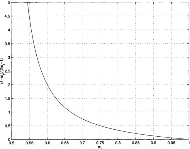
where P is the length of the original impulse response. The condition given by equation (3.19) states that if the ratio of the total energy in the portion of the impulse response not covered by the window to the total energy in the windowed impulse response is greater than 1-mr then iterative randomized sampling leads to an estimation error with lower variance 2mt-1e

equation (3.19) shows that IDTRS can never outperform LTI approximation techniques if

mr < 0.5. Figure 3-3 shows how the ratio 1-mr varies with mr

5 4.5 4 3.5 -3 E -2.5 E 1.51 1 0.5 0.55 0.6 0.65 0.7 0.75 0.8 0.85 0.9 0.95 1 m

Figure 3-3: Boundary Condition for the LMMSE Approximation Problem. IDTRS

Out-performs any LTI Approximation Technique if k e > 1-r

It is clear from Figure 3-3 that, since the length of the window is constrained by equation (3.20), and assuming the window is positioned optimally, i.e. around the region of the filter

with maximal energy, equation (3.19) cannot be satisfied if

Ih[n]l

single peak. A direct consequence of this is that if the filter of interest is a linear-phase low-pass filter and the goal is to minimize error variance, then the window method is a better approximation method than randomized sampling. However, if the Wiener filter impulse response has multiple peaks, i.e. its energy is spread out in time, and the desired number of non-zero taps in the approximate filter, M, is such that equation (3.19) is satisfied, then

U 0.5

- - - -.-. - - .. ..- --. - --. . .. .. . . .. . . .. .. . . . .-.-.-- -.-.- -.-.-. -.-- . -.-. .-- - - .-- - - -

.-- . - - ... ....- ...-. .. ...- .. . ...-. .

--it is better, in the mean-square sense, to use a long filter and --iteratively randomly sample it than use the best mean-square linear filter of length M.

3.2.3 Non-White r[n]

The truncated Wiener filter is the best length-M linear minimum mean-square estimator only if the received signal, r[n], is white. If r[n] is not white, then the optimal linear mean-square estimator needs to be computed every time M changes. This may not be desirable or even feasible in cases where resources are limited or if algorithm simplicity is of primary concern. In these cases, a straight-forward approach would be to truncate the Wiener filter or iteratively randomly sample it if the conditions in equation (3.19) are satisfied. Alternatively, the estimator could be decomposed into two systems with different resource allocations: a whitening filter implemented accurately, and a constrained Wiener filter (with limited resources) operating on the white data. In this case, the problem is similar to the one discussed in the previous section and the IDTRS method may lead to a better mean-square estimate than the best LTI approximation method.

3.3

Summary

This chapter exploited randomized sampling as a filter approximation technique. Results derived in Chapter 2 were used to compare IDTRS filter approximations to LTI approxima-tion techniques. Specifically, we compared the performance of both methods in the context of linear minimum mean-square estimation with complexity constraints was compared and conditions were derived, in the case of white data, where IDTRS lead to a better mean-square estimate than the best constrained linear mean-mean-square estimator. Scenarios where it would be desirable to use IDTRS even if the data is not white were also discussed.

Chapter 4

Low-Power Digital Filtering

In this chapter, we explore the use of randomized sampling as a way to reduce power consumption in a filtering context by examining the tradeoff between power savings and output quality. To this end, we first give a low-power formulation for randomized sampling by showing how setting some filter coefficients to zero can lead to powering down parts of the processor and therefore reducing the switching activity. Further savings can be obtained by slowing-down the computation in order to avoid processor idling time, and therefore reducing the voltage supply. Clearly, the additional savings due to scaling the voltage supply are not specific to randomized sampling but a consequence of reduced computation and have been already thoroughly examined [6]. However, some of these results will be re-derived in this chapter in order to quantify the tradeoff between power savings and output quality for the case of randomized sampling.

4.1

Low-Power Formulation

With the recent expanding interest in wireless systems, reducing power consumption is becoming an additional design factor along with size and speed. As discussed in Chapter 1, algorithmic approaches to low-power design are mainly concerned with reducing the switching power given by equation (4.1)

where Ci is the average capacitance switched per operation of type i corresponding to addition, multiplication, storage, or bus access. Ni is the number of operations of type i

performed per output sample, Vdd is the operating supply voltage, and

f,

frequency. In general, any discrete-time randomized sampling approach in a filtering context consists of reducing the average number of multiplications and additions performed per output sample. As a result, any discrete-time randomized sampling approach can be used in a low-power processing context where the power savings result from a reduction in Ni in equation (4.1).

x[n] N- h[n] -- y[n]

Figure 4-1: Original System.

Specifically, consider a time-domain implementation of the convolution illustrated by the system shown in Figure 4-1. If the filter, h[n], has length po, then a time-domain implementation of the convolution requires (po + 1) multiplications and po additions per output sample as can be seen in equation (4.2).

y[n] = h[O]x[n] + h[ljx[n - 1 + h[2]x[n - 2] + ... + h[po]x[n - po. (4.2)

Discrete-time randomized sampling of the impulse response can lead to power savings through both a lower switching activity (lower Nj) and a scaling of the voltage supply

(lower Vdd) which we examine separately in the next sections.

4.1.1 Switching Activity Reduction

Both DTRS of the impulse response and IDTRS using a sampling process with mean m,

consist of setting an average of (1 - mr) filter coefficients to zero prior to computing each

output sample. In the DTRS case, the same subset of filter coefficients is set to zero for all time whereas in the IDTRS case, the subset is different for each output sample. As a result, for both cases, mr(po + 1) multiplications and mrpo additions are required, on average, per

output sample, i.e. the number of multiplications and additions used per output sample is

reduced by a factor of (1 - mr) which corresponds to a similar reduction in the switching

activity. Since average switching power is a linear function of the amount of computation

required per output sample, a reduction by (1 - mr) in computation leads to a reduction

in power consumption by the same factor.

IN

h[O] x h[1] x h[2] x h[3] x h[n - 1] x h[n] x

MUX

OUT

Figure 4-2: FIR Filter Structure for Low-Power Filtering Using Discrete-Time Randomized Sampling. MUX is used as an abstraction to a collection of multiplexers.

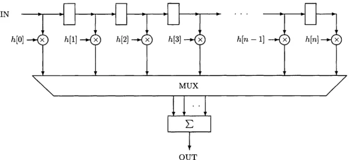
Figure 4-2 illustrates a low-power implementation for discrete-time randomized sam-pling. At each time point or clock cycle, a subset of the outputs of the multipliers is picked by a collection of multiplexers (abstracted by MUX in the figure), the remaining multiplica-tions are not performed therefore reducing computation. The chosen subset is then used as an input to an accumulator which performs the final addition to generate the output. Figure 4-3 shows an equivalent implementation where the powering down of a subset of the multi-plication branches is made explicit by the addition of switches for each branch. Branches that are powered down are not used by the adders. The normalized power consumption as a function of the mean, mr, of the sampling process is shown in Figure 4-4.

4.1.2 Supply Voltage Reduction

Figure 4-3 suggests yet a further reduction in power through an increase in the propagation delay which allows a reduction in the supply voltage while maintaining the same throughput

IN

h[O] -x h[l] x h[2] x h[3] x h[n

-

+4 +

OUT

Figure 4-3: FIR Filter Structure for Low-Power Filtering using Randomized Sampling.

as the initial system. Burd and Brodersen [4] note that if the clock-rate is equal to the increase of the critical path delay, then throughput is proportional to the number of parallel operations per clock cycle (concurrency) divided by the delay, i.e.:

Operations Concurrency

T second Delay (4.3)

In this case, delay refers to the time it takes to perform a multiplication. Most digital signal processing applications are real-time applications and as a result the throughput is fixed. In the filtering context of Figure 4-1, the number of parallel operations per clock cycle correspond to the number of multiplications per output sample which is equal to (po + 1) in the original system. Using the randomized sampling approximation method, the number of multiplication is reduced to mr(po + 1) and so is the amount of concurrency per clock cycle. It is thus clear from equation (4.3) that an increase in the delay by a factor of

1/mr will compensate for the decrease in the amount of concurrency and therefore the same

throughput could be maintained. In this context, there is no need to increase throughput, power reduction has higher priority. Chandrakasan et al. [6] have already explored the idea of lowering the voltage supply if less work needs to be done by developing an approach to minimize the energy dissipation per output sample in variable-load DSP systems. Here, we derive similar results and apply them to randomized sampling.