HAL Id: hal-02045757
https://hal.archives-ouvertes.fr/hal-02045757
Submitted on 22 Feb 2019
HAL is a multi-disciplinary open access
archive for the deposit and dissemination of
sci-entific research documents, whether they are
pub-lished or not. The documents may come from
teaching and research institutions in France or
abroad, or from public or private research centers.
L’archive ouverte pluridisciplinaire HAL, est
destinée au dépôt et à la diffusion de documents
scientifiques de niveau recherche, publiés ou non,
émanant des établissements d’enseignement et de
recherche français ou étrangers, des laboratoires
publics ou privés.
The Normal Graph Conjecture for Two Classes of
Sparse Graphs
Anne Berry, Annegret Wagler
To cite this version:
Anne Berry, Annegret Wagler. The Normal Graph Conjecture for Two Classes of Sparse Graphs.
Graphs and Combinatorics, Springer Verlag, 2018, 34 (1), pp.139-157. �hal-02045757�
(will be inserted by the editor)
The Normal Graph Conjecture for two classes of
sparse graphs
Anne Berry · Annegret K. Wagler
Received: date / Accepted: date
Abstract Normal graphs are defined in terms of cross-intersecting set fami-lies: a graph is normal if it admits a clique cover Q and a stable set cover S s.t. every clique in Q intersects every stable set in S. Normal graphs can be considered as closure of perfect graphs by means of co-normal products and graph entropy. Perfect graphs have been characterized as those graphs with-out odd holes and odd antiholes as induced subgraphs (Strong Perfect Graph Theorem, Chudnovsky et al. 2002). K¨orner and de Simone observed that C5,
C7, and C7are minimal not normal and conjectured, in analogy to the Strong
Perfect Graph Theorem, that every (C5, C7, C7)-free graph is normal (Normal
Graph Conjecture, K¨orner and de Simone 1999). Recently, this conjecture has been disproved by Harutyunyan, Pastor and Thomass´e. However, in this paper we verify it for two classes of sparse graphs, 1-trees and cacti. In addition, we provide both linear time recognition algorithms and characterizations for the normal graphs within these two classes.
Keywords Normal Graph Conjecture · 1-trees · cacti
A. Berry
LIMOS (UMR CNRS 6158), Universit´e Clermont Auvergne, Clermont-Ferrand
Campus Universitaire des C´ezeaux, 1 Rue de la Chebarde, 63173 Aubi`ere Cedex, France Tel.: +33 473 40 7769
Fax: +33 473 40 7639 E-mail: [email protected] A. Wagler
LIMOS (UMR CNRS 6158), Universit´e Clermont Auvergne, Clermont-Ferrand
Campus Universitaire des C´ezeaux, 1 Rue de la Chebarde, 63173 Aubi`ere Cedex, France Tel.: +33 473 40 5367
Fax: +33 473 40 5001
1 Introduction
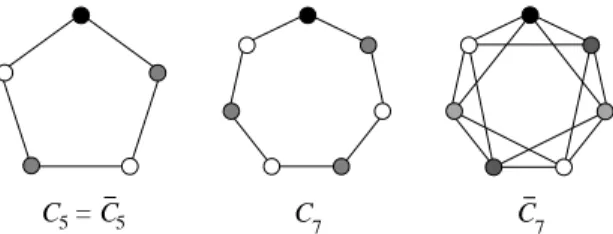
Normal graphs come up in a natural way in an information theoretic context by studying co-normal products [7] or graph entropies [4]. A graph G is normal if G admits cross-intersecting clique and stable set covers, called a valid pair (Q, S): a clique cover Q and a stable set cover S s.t. every clique in Q intersects every stable set in S. (A set is a clique (resp. stable set) if its nodes are mutually adjacent (resp. non-adjacent).) Figure 1 presents three normal graphs and their valid pairs. 2 1 3 2 3 1 2 3 1 1 3 2 3 1 2 1 3 1 2 2 3 2 1 2 3 3 2 1 1 3 1 2 3
Fig. 1 Three normal graphs and their valid pairs: bold edges indicate the clique covers, labels the cross-intersecting stable set covers
The class of normal graphs includes the well-studied perfect graphs, and the interest in normal graphs is caused by the fact that they form, in different ways, a weaker variant of perfect graphs.
Berge introduced the latter class in 1960, motivated from Shannon’s infor-mation-theoretic problem of finding the zero-error capacity of a discrete mem-oryless channel [14]. Shannon’s problem has a graph-theoretic formulation, re-garding the asymptotic growth of the maximum cliques in the co-normal prod-uct Gn of G = (V, E), where G2has V × V as node set and {(a
1, b1), (a2, b2) :
(a1, a2) ∈ E or (b1, b2) ∈ E} as edge set.
Berge [1] introduced perfect graphs as those graphs G, where the clique number ω(G′) equals the chromatic number χ(G′) for each induced subgraph
G′ ⊆ G (ω(G) denotes the size of a maximum clique in G, χ(G) the least
number of stable sets covering all nodes of G).
Berge observed that chordless odd cycles C2k+1with k ≥ 2, the odd holes,
and their complements, the odd antiholes C2k+1 with k ≥ 2, are graphs G
with ω(G) < χ(G), see Figure 2. (The complement G has the same node set as G but two nodes are adjacent in G iff they are non-adjacent in G.) This motivated Berge’s Strong Perfect Graph Conjecture: a graph G is perfect if and only if G is odd hole- and odd antihole-free. In a sequence of remarkable results, Chudnovsky et al. [3] finally turned the above conjecture into the Strong Perfect Graph Theorem.
Normal graphs are a closure of perfect graphs in terms of graph entropy [4,8,15] and taking co-normal products: K¨orner and Longo [7] showed that all co-normal products of a graph G are perfect only if G is the union of disjoint cliques. However, all co-normal products of normal (and, therefore, of perfect) graphs are normal by [6].
C 7 C 7
5
C = C5
Fig. 2 Small odd holes and odd antiholes
This motivated K¨orner and de Simone [9] to ask for a similarity of the two classes in terms of forbidden subgraphs. K¨orner [6] showed that an odd hole C2k+1 is normal if and only if k ≥ 4. By the invariance of normality
under taking complements, an odd antihole C2k+1 is also normal if and only
if k ≥ 4. C5, C7 and C7 are minimally not normal since all of their proper
induced subgraphs are perfect and, hence, normal. K¨orner and de Simone conjectured that there are no other minimally not normal graphs:
Conjecture 1 (Normal Graph Conjecture [9]) All graphs without a C5, C7, and
C7as induced subgraph are normal.
Note that the non-existence of C5, C7, and C7 in a graph is not necessary
to be normal (see the first two graphs in Figure 1), and a characterization of normal graphs by forbidden subgraphs is not possible (see [17]). So far, the Normal Graph Conjecture has been verified for webs [16] and line graphs [12]. In order to treat the Strong Perfect Graph Conjecture from a probabilistic point of view, Pr¨omel and Steger [11] asked for the relation of perfect and odd hole, odd antihole-free graphs with the same number of nodes. For that, they proved that almost all C5-free graphs are perfect. Since every (C5, C7, C7
)-free graph is C5-free, also almost all (C5, C7, C7)-free graphs are perfect and,
therefore, normal.
However, the Normal Graph Conjecture has been recently disproved by Harutyunyan, Pastor and Thomass´e [5]. Their proof is based on probabilistic arguments, showing the existence of a not normal graph with girth at least 8, i.e., without holes Ck of length k ≤ 7 (which also excludes C7since it contains
C3andC4), but without presenting an explicit counterexample.
Both results together imply that there are only few counterexamples and that they should be sparse (due to the large girth ≥ 8). This motivates our study of two classes of sparse graphs w.r.t. normality.
We start with a class of graphs having as many edges as nodes: A 1-tree is a connected graph G = (V, E) with |V | = |E| (obtained from a tree by adding one edge since trees are precisely the connected graphs with |V | − 1 = |E|). Hence, G contains exactly one cycle C (due to this property, 1-trees are also called unicyclic graphs). In other words, G can be obtained from the cycle C and certain trees by a sequence of node-identifications.
In Section 3, we characterize the normal 1-trees with the help of two results: a connected triangle-free graph is normal if and only if it has a so-called
nice edge cover [9] and the identification of two normal graphs in one node yields a normal graph again. The latter is a consequence from results on clique identification and normality in [17], see Section 2. We obtain that the only not normal 1-trees are either equal to a C7or contain a C5. This verifies the Normal
Graph Conjecture for the class of 1-trees (note: no C7can occur in a 1-tree, so
it suffices to show that (C5, C7)-free 1-trees are normal) and leads to a linear
time recognition algorithm for normal 1-trees.
We then use these results to treat the larger class of cacti in Section 4. A
cactus is a connected graph whose cycles are all edge-disjoint. Thus, a cactus
G= (V, E) with k cycles can be considered as a graph obtained from a tree by adding k edges in a certain way (thus cacti admit |V | − 1 + k edges) or, alternatively, as a graph obtained from k 1-trees by a sequence of node-identifications.
We can, therefore, apply the characterization of normal 1-trees from Section 3 in order to decide whether or not a cactus is normal: As the class of normal graphs is closed under node identification (see Section 2), a cactus is normal if it can be obtained by identifying normal 1-trees in nodes; this verifies the Normal Graph Conjecture for cacti, as in particular all (C5, C7)-free cacti are
normal.
Moereover, there also exist normal cacti containing a C5 or a C7, so our
further goal is to recognize normal cacti. As one can obtain a normal graph by identifying certain not normal graphs in one node, see Section 2 again, we examine in detail when a graph constructed by identifying two 1-trees in a node can be normal. This enables us to design an algorithm that decides for a cactus, given a decomposition into1-trees, in linear time whether or not it is normal. In addition, we achieve a characterization of normal cacti.
We close with some concluding remarks and discuss consequences and some future lines of research.
Parts of the here presented results appeared without proofs in [2].
2 Clique identification and normal graphs
A graph G arises by identification of two disjoint graphs G1and G2in a clique
if there are cliques Q1 ⊆ G1 and Q2 ⊆ G2 with |Q1| = |Q2| and a bijection
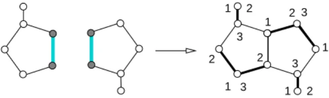
φ: Q1→ Q2 identifying every node v ∈ Q1 with φ(v) ∈ Q2, see Figure 3.
In this section, we discuss how normal graphs can be obtained by clique identification. The first two graphs in Figure 1 are examples of normal graphs, constructed by identifying a non-normal C5 and C7 with two edges and one
edge, respectively. Figure 3 shows another normal graph obtained by identify-ing two non-normal graphs in an edge.
However, the non-normal building blocks in these examples are not too far from being normal which shows in particular that it obviously suffices if the nodes in the common clique are covered in one of the two building blocks. This suggests to relax the condition of normality for the building blocks as follows. Let G be a graph such that G has a stable set cover S, G − Q′ has
1 2 3 1 1 1 1 2 2 2 2 3 3 3
Fig. 3 Identifying two non-normal graphs in an edge: bold edges indicate the clique cover, labels the cross-intersecting stable set cover of the resulting normal graph
a clique cover QQ′, for some clique Q′, and S and QQ′ are cross-intersecting.
We call such a graph G nearly normal, (QQ′,S) a nearly valid pair of G, and
Q′an unnormal clique of G. Figure 4 shows examples of nearly normal graphs
together with their nearly valid pairs and unnormal cliques. 2 2 2 1 1 3 3 3 2 1 1 3 1 3 2 2 1 3 2 2 2 2 2 2 1 1 1 3 3 3 3 3 1
Fig. 4 Nearly normal graphs: the gray-shaded nodes induce the unnormal cliques Q′, bold
edges indicate the clique covers QQ′, labels the cross-intersecting stable set covers
It was shown in [17] that this weaker form of normality suffices for con-structing a normal graph by clique identification, provided the involved stable set covers are suitable.
Lemma 1 [17] Construct G by identifying two nearly normal graphs G1 and
G2 in a clique Q∗ and let Q1, Q2 ⊆ Q∗ be disjoint unnormal cliques. The
resulting graph G is normal if there exist nearly valid pairs (QQi(Gi), S(Gi)) for i = 1, 2 satisfying at least one of the following conditions.
(1) S(Gi) contains a stable set S with S ∩ Q∗= ∅ for i = 1, 2;
(2) S(Gi) contains no stable set S with S ∩ Q∗= ∅ for i = 1, 2;
(3) S(G1) contains a stable set S with S ∩ Q∗= ∅ but S(G2) does not, and Q1
is non-empty (or vice versa).
Lemma 1 provides sufficient conditions to obtain a normal graph via clique identification, but it is not yet clear whether these conditions are also
nec-essary. However, condition (1) of Lemma 1 is certainly satisfied if Q∗ is a
non-maximal clique in Gifor i = 1, 2: In order to cover a common neighbor v
of all nodes in Q∗, S(Gi) has to contain a stable set S with v ∈ S and, thus,
S∩ Q∗= ∅.
Corollary 1 The class of normal graphs is closed under identification in non-maximal cliques.
In particular, this is the case if Q∗ consists in a single (but not isolated)
node only. Thus, the class of normal graphs is closed under node-identification. As we have seen that we can construct normal graphs by identifying two unnormal ones in a clique (as in Figure 3), a natural question is whether there exist further ways to construct normal graphs by clique identification. The next lemma from [17] gives an answer showing that the normality or near-normality of the building blocks is required if the resulting graph is supposed to be normal.
Lemma 2 [17] Let G be a normal graph obtained by identifying two graphs G1 and G2 in a clique Q∗.
(1) If G admits a valid pair (Q, S) such that S contains no stable set avoiding Q∗, then G
1 and G2 are normal;
(2) If G admits a valid pair (Q, S) such that S contains a stable set avoiding Q∗, then G1 and G2 are nearly normal with unnormal cliques Q∗
1 and Q∗2
such that Q∗
i ⊆ Q∗ and Q∗1∩ Q∗2= ∅.
Note that in case (2) of the lemma, Q∗
1 and Q∗2 may be empty (such that
G1and G2become normal), but that the weaker condition that G1and G2are
nearly normal already suffices, provided Q∗
1 and Q∗2are disjoint. However, we
cannot obtain normal graphs by identifying two non-normal graphs in a node (as the unnormal cliques Q∗
1, Q∗2⊆ Q∗ cannot be disjoint if |Q∗| = 1). We call
a nearly normal graph almost normal if its unnormal clique consists in one node only. Except the C5(whose only possible unnormal clique has size two),
all the graphs in Figure 4 are examples of almost normal graphs. We finally obtain the following result which is crucial for our purposeas an immediate consequence of Lemma 2:
Theorem 1 Construct a graph G by identifying two graphs G1 and G2 in a
node q∗, G is normal if and only ifoneof the following conditions holds:
(1) G1 and G2 are normal;
(2) G1 is normal and G2 almost normal with unnormal node q∗, or vice versa.
Indeed, condition (1) of the theorem is satisfied if in Lemma 2 either case (1) occurs or case (2) with Q∗
1 and Q∗2 empty; condition (2) of the theorem is
satisfied if case (2) of Lemma 2 occurs where one of G1and G2is normal, the
other is almost normal with unnormal clique {q∗} = Q∗.
3 The Normal 1-Trees
In this section we characterize the normal 1-trees, verify the Normal Graph Conjecture for such graphs, and provide a linear time recognition algorithm for normal 1-trees.
Recall that a 1-tree G is a connected graph containing exactly one cycle C, i.e., G can be obtained from the cycle C and certain trees by a sequence of
node-identifications. In order to characterize the normal 1-trees we use Theo-rem 1 and the result that a connected triangle-free graph is normal if and only if it has a so-called nice edge cover [9], as defined below.
Let G = (V, E) be a graph and F be a minimal edge cover of G, i.e., an inclusion-wise minimal set F ⊆ E s.t. every node in V is the endnode of some edge in F (note that a minimal edge cover is the union of node-disjoint stars). Consider a (not necessarily chordless) odd cycle C in G and the distribution of the edges of F alongside the cycle C. We say that a node v of C is even w.r.t. F if v is the endnode of either none or two edges in F ∩ E(C). Since C is an odd cycle, C has an odd number of even nodes. An edge cover of a graph G is called nice if it is minimal and every odd cycle in G has at least three even nodes.
For example, the bold edges of all three graphs in Figure 1 form nice edge covers, whereas the graphs in Figure 4 do not admit any nice edge cover.
K¨orner and de Simone showed in [9] that the occurrence of nice edge covers is sufficient for a graph to be normal. In particular, they characterized the triangle-free normal graphs as follows:
Theorem 2 [9] A connected triangle-free graph is normal if and only if it has a nice edge cover.
Let G1+vG2denote the graph obtained from G1and G2 by identification
in the node v. For instance, the second graph in Figure 4 equals C5+v K2,
obtained from a C5and a K2by node identification; the third graph in Figure
4 equals (C5+vK2) +v′K2, obtained from C5+vK2and K2 by identification
in another node of the C5.
We characterize the normal 1-trees with the help of Theorem 1 and Theo-rem 2 as follows.
Theorem 3 A 1-tree G is not normal if and only if one of the following conditions holds.
(1) G = C5.
(2) G = C5+vT where T is a tree.
(3) G = (C5+vT) +v′T′ where T, T′ are trees and v, v′ two non-consecutive nodes of the C5.
(4) G = C7.
Proof A 1-tree G is obtained from a tree by adding one edge. Hence, G contains
exactly one chordless cycle C and G − C is a (possibly empty) forest. Thus, G can be obtained from C and certain trees by a sequence of node-identifications. We prove, dependent on the length of C, whether G is normal or not.
Claim If C 6= C5, C7then G is normal.
Every hole C 6= C5, C7is normal. Hence G can be obtained from normal graphs
by a sequence of node-identifications and is, thus, normal by Theorem 1(1). 3 It remains to consider the cases C = C5 and C = C7. Let G5 denote the
Claim If C = C5then G is normal if and only if G contains the graph G5 as
subgraph.
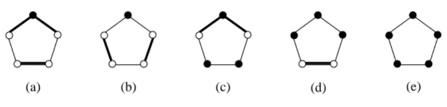
Gis triangle-free in both cases, hence G is normal if and only if it admits a nice edge cover by Theorem 2. Every minimal edge cover F of G uses at most three edges of the C5. All possible types of F ∩C5are shown in Figure 5 (edges
in F ∩ C5 are drawn with bold lines, even nodes w.r.t. F are black-filled).
F is nice if and only if two consecutive nodes v, v′ of the C
5are not covered
by the edges in F ∩ C5(the types (c), (d), and (e)). In order to cover the nodes
v, v′ by F, there must exist non-empty trees T, T′ identified with the C5 in v
resp. v′. Thus, F is nice if and only if G contains the graph G5 as subgraph.
(Note that G = C5 is not normal. If G = C5+vT or G = (C5+vT) +v′T′
where v, v′ are two non-consecutive nodes of the C5, then F has to be of type
(a) or (b) and is, therefore, not nice.) 3
(a) (b) (c) (d) (e)
Fig. 5 Possible types of F ∩ C5
Claim If C = C7then G is normal if and only if G 6= C7.
If G = C7then G is clearly not normal. Otherwise, G can be obtained from the
C7 and certain trees by a sequence of node-identifications. The C7 is almost
normal and all of its nodes are unnormal. Thus identifying the C7with a
(non-empty) tree in a node yields a normal graph by Theorem 1(2), adding further trees maintains normality by Theorem 1(1). Hence G is normal. 2
Thus, the non-normal 1-trees are all not (C5, C7, C7)-free by Theorem 3
which implies:
Corollary 2 The Normal Graph Conjecture is true for 1-trees.
As there are obviously normal 1-trees admitting a cycle of length 5 or 7, we next address the question of recognizing normal 1-trees.
To find the cycle in a 1-tree G = (V, E) as first step, we will use Algorithm LexBFS [13]1. LexBFS is a specialized Breadth-First Search, which numbers
1
Although a simple DFS with a ’father’ function could be used with the same time complexity, LexBFS provides us an elegant way to directly determine the studied cycle as well as its nodes.
the nodes from n = |V | to 1; each node x obtains a label, denoted by lex(x), which is the decreasing list of the neighbors of x with a higher number than that of x. At each step, a node of lexicographically largest label is chosen to be numbered. A node will be referred to by its number, and when a node x has a label of size 1, f ather(x) will refer to the node in the label.
When the input graph has only one cycle, all the nodes obtain a label of size 1, except the node which ’closes’ a cycle, whose label is of size 2. To find the corresponding cycle C, we can use the double label, which yields the next 2 nodes on C; we then go on to take the lowest numbered node between these two: its label yields the next node on C, and so on, until we find a node already in C, which will be the ’root’ of C in the tree induced by the LexBFS numbering. The algorithm can stop as soon as more than 7 nodes of the cycle have been found, as the graph is certain to be normal.
Theorem 4 Given a 1-tree G = (V, E), Algorithm 1 decides in O(|V |) whether or not G is normal.
Proof Since G is a 1-tree (i.e., G is connected and has one cycle), Algorithm
1 finds at some point an already labeled neighbor x of the current node y and assigns a double label lex(x) = (y, z) (this can be done in O(|V |) since at most |V | = |E| edges have to be tested). The edge xy closes a cycle C, and it remains to test whether C has length 5 or 7 and the conditions of Theorem 3 are satisfied or not. For that, it suffices to go from y and z 5 steps backwards along the unique paths towards the root node r (always passing from a node to its father), looking for a common node of the paths: if C has length 5 or 7, it has been found that way, and the conditions of Theorem 3 decide about normality (which can be tested in constant time). In all other cases (i.e., if C has length 3, 4, 6, 8 or no cycle has been found yet), G is normal. 2
Remark 1 Algorithm 1 can be turned into a robust algorithm that in addition
decides, still in linear time, whether the input graph G = (V, E) is a 1-tree. For that, the graph has to satisfy |V | = |E| and has to be connected. This can be tested by running BFS until no further nodes can be reached (then G is a 1-tree if and only if T contains all nodes from V and exactly one edge xy is not included).
4 The Normal Cacti
In this section we study cacti, i.e., graphs with edge-disjoint cycles. Since a cactus G with k cycles can be considered as a graph obtained from a tree by adding k edges, we can alternatively obtain G from k 1-trees by a sequence of node-identifications.
As we have characterizations of both normal graphs obtained by node-identification (Theorem 1) and normal 1-trees (Theorem 3) from the previous sections, it is natural to decompose a cactus G accordingly: we have to choose
Algorithm 1 (1-tree normality) input : A 1-tree G = (V, E).
output: An answer to the question: ’Is G normal?’.
Initialize all node labels lex() as empty,for all nodes the LexBFS order α() as empty;
for i = n downto 1 do
Choose a node x with maximum label; α(x) ← i;
foreach unnumbered neighbor of x doAppendito lex(x); if |lex(x)| = 2 then
Let j1 and j2be the nodes of lex(x), with j1> j2;
C← {i, j1, j2}; c ← 3; d ← 0; D ← ∅;
if degree of i in G > 2 then D ← D + {i} ; d ← d + 1; if degree of j1 in G > 2 then D ← D + {j1} ; d ← d + 1; if degree of j2 in G > 2 then D ← D + {j2} ; d ← d + 1; repeat j1← f ather(j1); if degree of j1 in G > 2 then D ← D + {j1};d ← d + 1; C← C + {j1};c ← c + 1; if j1> j2 then k ← j1;j1← j2; j2← k;
if c > 7 then Return(’G is normal’); until f ather(j1) ∈ C;
r← f ather(j1); //A small cycle C of root r has been found;
if c 6= 5 and c 6= 7 then Return(’G is normal’); if c = 7 then
if n=7 then Return(’G is not normal’) else Return(’G is normal’)
if c = 5 then
if |V | = 5 or d = 0 or d = 1 then Return(’G is not normal’) else
if d = 2 and the nodes in D are not adjacent then Return(’G is not normal’ )
else Return(’G is normal’)
a set of articulation points in G s.t. each building block contains exactly one cycle (and is, thus, a 1-tree). We denote the building block of cycle C by B(C). If all these blocks B(C) of G are normal, then G is clearly normal due to Theorem 1. This holds particularly if none of the cycles C in G has length 5 or 7 by Theorem 3; hence we have:
Corollary 3 The Normal Graph Conjecture is true for cacti.
As there are obviously normal cacti admitting a cycle of length 5 or 7, our further goal is to find a way to decide whether or not a cactus is normal.
For that, we introduce the block-tree of a cactus as follows. For a cactus G = (V, E) with k cycles, we call a set A ⊆ V of articulation points valid if A can be used to decompose G so that the resulting building blocks B(C) contain exactly one cycle C each.
Hence, using a valid set of articulation points decomposes a cactus in as many 1-trees as it has cycles. We obtain the block-tree T (G, A) = (A ∪ B, L)
of G by taking as nodes a valid set A of articulation points and the set B of the resulting building blocks B(C) of G and joining two nodes of T (G, A) if and only if one corresponds to an articulation point q ∈ A and the other one to a block B(C) with q ∈ B(C).
By construction, T (G, A) is a tree as it is bipartite and has no cycle. We call a leaf of T (G, A) an endblock of G and say that two blocks of G are adjacent if they share an articulation point in A. Figure 6 shows a cactus G and a block-tree T (G, A) (the black nodes of G are used as articulation points).
C’ C C" q q’ B(C") q’ B(C) B(C’) q
Fig. 6 A cactus and a block-tree
The main idea is to design an algorithm that, given a cactus G, – finds a valid set A ⊆ V and constructs the block-tree T (G, A), – decides the normality status of each block B(C),
– shrinks T (G, A) iteratively by deleting an endblock B(C) and deciding how normal the remaining graph is.
We next explain in detail a procedure to construct A and the block-tree T(G, A), how to decide the normality status of each block B(C), and of the remaining graph after deleting an endblock.
Constructing a block-tree To construct a block tree, we will again use
algo-rithm LexBFS. A node will be referred to by its number. Each node will be assigned 2 labels: its LexBFS label lex(x), and its block label block(x) which is the list of block numbers which x belongs to. At the end, block(x) has size at least 2 if x is in the set A of valid articulation points. When a node x has a label of size 1, f ather(x) will refer to the node in the label.
In order to test for normality, we will also, while defining a cycle C, collect the set C of nodes of C and the subset D of nodes of C whose degree in G is 3 or more. These information will be added to the block, as well as its status of ’normal’ when it can be determined during the construction of the block tree. A Boolean f irstcycle will avoid starting a new block when the very first cycle is encountered.
Theorem 5 Given a cactus G = (V, E), Algorithm 2 constructs a block-tree of G in O(|V |).
Proof LexBFS, like any BFS, induces a spanning tree T of the input graph G.
Algorithm 2 (Block tree construction) input : A cactus G = (V, E).
output: ’G fails to be normal’ or: a block tree T (G, A) = (A ∪ B, L) of G, with information in each block, a set A of valid articulation points of G, a numbering σ of V , the function block() on V containing the numbers of the blocks each node belongs to.
Initialize all node labels as empty; f irstcycle ← 1; t ← 1, n ← |V |; for i = n downto 1 do
Choose a node x with maximum lex label; σ(x) ← i; Add t to block(x); foreach unnumbered neighbor y of x do
Add i to lex(y); if |lex(x)| = 2then
j1, j2∈ lex(x), with j1< j2; C ← {i, j1, j2}; D ← ∅;
if degree of i in G > 2 then D ← D + {i}; if degree of j1 in G > 2 then D ← D + {j1}; if degree of j2 in G > 2 then D ← D + {j2}; repeat j1← f ather(j1); C ← C + {j1}; if degree of j1 in G > 2 then D ← D + {j1}; if j1> j2 thenu← j1; j2← j1; j1← u; until f ather(j1) ∈ C;
r← f ather(j1); if f irstcycle = 0 then
t← t + 1;// a new block is defined; Add t to block(r);
foreach node y of C − {r} do
if |block(y)| = 1 then block(y) ← t;
else Replace the first entry in block(y) with t; A← A ∪ {r}; B ← B ∪ {Bt}; L ← L ∪ {{r, Bk}, {r, Bt}};
else
A← {r}; B ← {Bt}; L ← ∅; f irstcycle ← 0;
Add C and D as information to block Bt;
if |C| 6= 5, 7 then Mark Bt as normal;
if (|C| = 5) and (|D| = 0 or |D| = 1) or (|C| = 7 and |V | = 7) then Return(’G fails to be normal’).
1. When G is a cactus, the only edges of G which are not in T are those which close a cycle; clearly, these nodes will obtain a label of size 2. Let us consider such a cycle C; the node x with a double label is chosen to be numbered when all the nodes of C have been numbered, thus x is the lowest-numbered node of C; the highest-numbered node y of C is its root in T , and unless y = n, y will be a valid articulation point, separating any neighbor v of y with v > y from C \ {y}. (Note that n may also be an articulation point, separating the nodes of two cycles).
When the label is not double, the newly numbered node is added to the highest-numbered block which its father belongs to. Algorithm 2 starts a new building block Bt each time a cycle C is closed and defined; the
highest-numbered node is added to the block tree and to the set A of valid articulation points, with the possible exception of node n; the block labels of the nodes of C are updated: t is added to the block label of the root of C; for the other
nodes of C, if the node belongs to only 1 block, its block number is changed to the new block number t; if a node v of C belongs to more than 1 block, then its first block entry is changed to t (by construction, the other block entries correspond to other blocks which t is the root of).
The normality tests define as normal any block whose cycle is not of length 5 or 7. The graph is found to be not normal when either the graph is a C5 or
a C7, or when the current block contains a C5 with only 1 neighbor.
LexBFS runs in linear time [13]; a cactus has O(|V |) edges; defining the cycles costs at most |V | as the cycle edges are traversed only once; thus Algo-rithm 2 runs in linear O(|V |) time. 2
Deciding the normality status of blocks Since each block B(C) is a 1-tree by
construction, Theorem 3 characterizes whether it is normal or not. In view of Theorem 1, we have to distinguish the different not normal blocks: it is important to determine whether a not normal block B(C) is almost normal and to specify its unnormal nodes.
For that, we denote the set of possible unnormal nodes of an almost normal block B(C) by U (C) and notice that all of them lie on C: Any valid minimal clique cover of a cactus G uses edges and triangles only, maintaining the notion of even nodes for odd cycles C with length ≥ 5. An unnormal node q of B(C) is not covered by the clique cover Qq of a nearly valid pair (Qq,S) of B(C),
but it has to be covered by a clique outside B(C) to become an even node of the cycle C.
As an immediate consequence of Theorem 3 and the possible nearly valid pairs of unnormal 1-trees in Figure 4, we obtain the following proposition. Proposition 1 A block B(C) with cycle C is
(1) not (almost) normal if B(C) = C5;
(2) almost normal with U (C) = N (v) ∩ C if C = C5 and B(C) = C5+vT
where T is a tree;
(3) almost normal with U (C) = C \ {v, v′} if C = C5 and B(C) = (C5+v
T) +v′ T′ where T, T′ are trees and v, v′ are two non-consecutive nodes of the C5;
(4) almost normal with U (C) = C if B(C) = C7;
(5) normal otherwise.
Proof As any block B(C) is, by construction, a 1-tree, we distinguish according
to Theorem 3 the following cases.
1. C = C5: Then B(C) is normal if and only if B(C) contains the graph G5as
subgraph (due to the second claim in the proof of Theorem 3). We consider as subcases the three cases of Theorem 3 where B(C) is not normal and check whether B(C) is almost normal:
1.1 B(C) = C5: Then B(C) is not almost normal (since the only possible
1.2 B(C) = C5+vT where T is a tree: Then B(C) is almost normal and
the two neighbors of v are the possible unnormal nodes (see Figure 4), which proves (2).
1.3 B(C) = (C5+vT) +v′ T′ where T, T′ are trees and v, v′ are two non-consecutive nodes of the C5: Then B(C) is almost normal and any
neighbor of v or v′ is a possible unnormal node (see Figure 4), which
proves (3).
2. C = C7: Then B(C) is normal if and only if B(C) 6= C7by Theorem 3. If
B(C) = C7, then B(C) is not normal, but almost normal and all its nodes
are possible unnormal nodes (see again Figure 4), which proves (4). 3. C 6= C5, C7: Then B(C) is normal by Theorem 3 (as all not normal 1-trees
contain C5or C7).
Hence, (1)-(4) are exactly the cases when B(C) is not normal (an if B(C) is almost normal, the possible unnormal nodes are identified). In all other cases (i.e., if C = C5 and B(C) contains G5, if C = C7 but B(C) 6= C7, or if
C6= C5, C7) B(C) is normal, which proves (5).
Shrinking a cactus by removing endblocks To iteratively shrink (the block-tree
of) a cactus G by removing an endblock B(C), we use the following idea based on Theorem 1: If B(C) does not satisfy any of the theorem’s conditions, then Gis not normal. Otherwise, G is normal if and only if the graph that results from G by either removing B(C) or collapsing a normal endblock B(C) into a K2 (i.e., into a smaller normal graph)is normal.
Consider a cactus G and a block-tree T (G, A). For an endblock B(C) of T(G, A) and (one of) its adjacent block(s) B(C′) with common node q ∈ A,
we denote by G − B(C) (resp. G − B(C) + e) the graph obtained by removing B(C) maintaining q (resp. by replacing B(C) by an edge e attached to q).
As an immediate consequence of Theorem 1 combined with Proposition 1, we infer the normality of G after removing B(C):
Corollary 4 Let G be a cactus with block-tree T (G, A), B(C) an endblock and
B(C′) an adjacent block with common node q ∈ A.
(1) If B(C) and B(C′) are normal, then G is normal if and only if G − B(C)
is normal.
(2) If B(C) is normal and B(C′) not, then G is normal if and only if G −
B(C) + e is normal.
(3) If B(C) is almost normal and q ∈ U (C), then G is normal if and only if G− B(C) is normal.
(4) If B(C) is almost normal and q 6∈ U (C) or if B(C) = C5, then G is not
normal.
While conditions (1), (3) and (4) are immediate consequences of Theorem 1 and Proposition 1, we note the following to justify condition (2): If B(C) is normal but B(C′) not, then G = B(C) +q(G − B(C)) is normal by Theorem 1
(in B(C′)). This is the case if and only if K2+q(G − B(C)) = G − B(C) + e
is normal (which also follows from Theorem 1 since K2 is normal so that the
same conditions for G − B(C) apply in both cases).
The above corollary enables us to shrink a cactus starting from endblocks, keeping normality of the input graph or deciding that G is not normal. Thereby, the cases (1) and (3) allow us to simply remove B(C), (4) provides sufficient conditions that G is not normal, and (2) allows us to maintain or change the normality status of the remaining block B(C′) + e = K2+qB(C′) as follows:
Lemma 3 Let G be a cactus with block-tree T (G, A), B(C) a normal endblock and B(C′) an adjacent block with common node q ∈ A.
(1) If B(C′) is almost normal and q ∈ U (C′), then B(C′) + e is normal in
G− B(C) + e.
(2) If B(C′) is almost normal and q 6∈ U (C′), then B(C′) + e remains almost
normal with U (C′) in G − B(C) + e.
(3) If B(C′) = C5, then B(C′) + e is almost normal with U (C′) = N (q) ∩ C′
in G − B(C) + e.
For the algorithmic process, however, it suffices to shrink the block-tree of a cactus by removing an endblock B(C) and, if necessary, updating the normality status of B(C′) according to Lemma 3.
Example 1 Reconsider the cactus G and its block-tree T (G, A) depicted in
Figure 6. Initially, we have the following normality status for its blocks: – B(C) is almost normal with q ∈ U (C) (Proposition 1(2)),
– B(C′) = C5is not normal (Proposition 1(1)),
– B(C′′) is normal (Proposition 1(5)).
We apply Algorithm 3 and notice that none of the sufficient conditions for Gbeing (not) normal is satisfied. Hence, we proceed with step “shrink” and select one of the two endblocks B(C) and B(C′′) of T (G, A).
If B(C) is selected, then B(C′) is its only adjacent block with common node
q∈ A. None of the two conditions to update the normality status of B(C′) is
satisfied, so we only remove B(C) and q from T (G, A). The subsequent test for sufficient conditions reveals that B(C′) = C5 is now an endblock, hence
the decision is “not normal” according to Corollary 4 (4).
On the other hand, if B(C′′) is selected, then B(C′) is its only adjacent
block with common node q′ ∈ A. The second condition is satisfied, hence
B(C′) is updated as almost normal with U (C′) = N (q′) ∩ C′; B(C′′) and q′
are removed from T (G, A). The subsequent test for sufficient conditions reveals that now all blocks are not normal, hence the decision is “not normal” due to Theorem 1.
In both cases, the algorithm finds the correct answer “not normal”. Theorem 6 Given a cactus G = (V, E), Algorithm 3 decides in O(|V |) whether or not G is normal.
Algorithm Block Status
input : A cactus G = (V, E), a block tree T (G, A) = (A ∪ B, L) of G, with t the number of blocks, computed by Algorithm 2, with information in each block B(C), with C the cycle of block B(C).
output: Each block B(C) has status information status(B(C)) which is not normal, almost normal or normal; almost normal blocks have set U (C), the set of possible unnormal nodes on cycle C of the block; N ormal contains the number of normal blocks, N onN ormal contains the number of not normal and almost normal blocks.
Initialize N ormal ← 0 ; N onN ormal ← 0 ; for i=1 to t do
C← cycle of block B(C); switch |C| do case 7
if |B| = 7 then
status(B(C)) ← almost normal ; N onN ormal ← N onN ormal + 1; U(C) ← C ;
else
status(B(C)) ← normal ; N ormal ← N ormal + 1 ; case 5 K← ∅; foreach node x in C do if degree of x in B(C) is > 2 then K← K + {x} ; if |K| ≤ 1 then if |K| = 1then v← node of K ; U (C) ← NG(v);
status(B(C)) ← almost normal ; else
status(B(C)) ← not normal ; N onN ormal← N onN ormal + 1 else
if |K| = 2 then v, v′← nodes of K;
if vv′ is not an edge of G then
U(C) ← C − K; status(B(C)) ← almost normal ; N onN ormal← N onN ormal + 1;
else
status(B(C)) ← normal ; N ormal ← N ormal + 1 ;
otherwise
status(B(C)) ← normal ; N ormal ← N ormal + 1 ;
Proof For a given cactus G, Algorithm 2 constructs in linear time a valid set
A of articulation points and the corresponding block-tree T (G, A) = (B ∪ A, L). By construction, every block B(C) ∈ B is a 1-tree, so the(easy to test) conditions of Proposition 1 determine its normality status (equals C5 and is
not normal, is almost normal with U (C), is normal); Theorem 3 guarantees that all possible cases are considered. These tests can be performed at no extra cost while creating the blocks of G.
Algorithm 3
input : A cactus G = (V, E), a block tree T (G, A) = (A ∪ B, L) of G, with t the number of blocks, computed by Algorithm 2, with information in each block B(C), with C the cycle of block B(C), and the status and sets U (C) computed by Algorithm Block Status, as well as Normal and NonNormal. output: An answer to the question: ’Is G normal?’
for i=t to 2 do //test;
if N ormal = i then Return(Yes); if N onN ormal = i then Return(No); B(C) ← block of number i;
if status(B(C)) is not normal then Return(No); if B(C) is a C5 then Return(No);
if status(B(C)) is almost normal and q 6∈ U (C) then Return(No); //update;
q← father node of block B(C) in block tree; C ← cycle of block B(C) ; B(C′) ← choose the adjacent block to B(C) of highest number ;
if B(C) is normal and B(C′) is almost normal and q ∈ U (C′) then
status(B(C′)) ← normal ;
if B(C) is normal and B(C′) = C5then
status(B(C′)) ← almost normal ; U (C′) ← N (q′) ∩ C′;
//shrink;
Remove B(C) from B and edge B(C)q from L; if q has degree 1 then remove q from A; if B1 is normal then Return(Yes);
else
Return(No);
Next, if all blocks are normal (resp. not normal), then Theorem 1 guar-antees that the whole graph is normal (resp. not normal). If one endblock B(C) satisfies condition (4) of Corollary 4 (i.e., if B(C) is almost normal and q 6∈ U (C) or if B(C) = C5), then G is not normal (since both conditions of
Theorem 1 fail).
If none of these sufficient conditions applies, it is necessary to choose an endblock B(C); this is done by choosing the remaining block which was de-fined last by Algorithm 2, which is an endblock by construction as a depth-first search on a tree ends on a leaf; an adjacent block B(C′) is then chosen.
Corol-lary 4 guarantees that the graph obtained by removing the endblock B(C) is normal if and only if G is normal. In the two tested cases, the normality status of the adjacent block B(C′) can be augmented according to Lemma 3.
Eventually, B(C′) becomes an endblock after removing B(C).
At the end of step “shrink”, we have the same situation as after the initial step and have to repeat both the tests for sufficient conditions and, if they fail, again step “shrink” for the next block.
The block-tree shrinks in each iteration, so that at latest after |B| − 1 iterations a decision can be made (as only one block is left). Corollary 4 and Lemma 3 guarantee that the current normality status of the remaining block corresponds to that of G.
To efficiently perform the tests and the selection of an endblock, counters for the number of normal and not normal blocks are used. Then, step “shrink” defines an endblock and an adjacent block, performs two easy tests and updates the normality status of B(C′), if necessary. The tests for condition (4) of
Corollary 4 has to be redone only for the new endblock. All this can be clearly done in linear time. 2
Finally, to obtain a characterization when a cactus G is normal, recall that a triangle-free graph is normal if and only if it has a nice edge cover [9] and notice that triangles occur in a cactus only as or in normal blocks. This motivates the construction of a triangle-free graph G∆obtained from a cactus
Gwhich is normal if and only if G is:
Theorem 7 Let G be a cactus and G∆ be a graph obtained from G by
con-tracting exactly two nodes from each triangle of G. Then G is normal if and only if G∆ is normal if and only if G∆ has a nice edge cover.
Proof Consider a cactus G and a graph G∆ constructed as above.
Claim 1. G∆ is a triangle-free cactus.
In G∆, none of the triangles of G remains by construction. Since all cycles
of G are edge-disjoint, the construction does neither create new triangles, nor cycles sharing an edge. 3
By Claim 1, we can apply Algorithm 2 and 3 also to G∆. In order to show
that Algorithm 3 applied to G and G∆returns the same output, we next
con-sider the normality status of a block B(C) with adjacent triangle ∆ in G and after the contruction in G∆. We have:
Claim 2. Let B(C) be a block and ∆ be a triangle sharing a nodeqwith B(C) in G and e be the edge in G∆obtained by contracting ∆. Then B(C) +q∆is
as normal as B(C) + e and the sets of unnormal nodes are equal.
This can be easily seen by simple case analysis for all possible normality sta-tusof B(C) according to Proposition 1 and observations as in Corollary 4 and Lemma 3. 3
Now, apply Algorithm 3 to G and G∆. Notice that the obtained
block-trees can be equal only if G is triangle-free; otherwise T (G∆, A∆) contains
less blocks than T (G, A).
For the test of sufficient conditions, we have: On the one hand, – if all blocks of G are normal, then all blocks of G∆are normal;
– if all blocks of G∆ are normal, but not all of G, then for each not normal
block B(C) of G, there is an attached triangle ∆ such that combining B(C) and ∆ yields a normal block.
In both cases, the output is “normal” for G and G∆. On the other hand,
– if all blocks of G are not normal, then G is triangle-free and G = G∆;
– if all blocks of G∆ are not normal, but not all of G, then each triangle ∆
of G is attached to a not normal block B(C) such that combining B(C) and ∆ in yields a not normal block;
– if an endblock of T (G, A) satisfies Corollary 4.(4), so does a corresponding endblock of T (G∆, A∆).
In all cases, the output is “not normal” for G and G∆.
Finally, contracting two nodes of a triangle can be seen as shrinking T (G, A) and Claim 2 guarantees that the outcome is the same. This proves that G is normal if and only if G∆is, and the remaining assertion follows from [9] since
G∆is triangle-free. 2
Remark 2 For a given cactus G, the triangle-free cactus G∆ is not unique
as there are three choices for the contruction of two nodes per triangle ∆ in G. Similarly, during the process of Algorithm 3, neither the construction of the block-tree T (G, A) of G is unique (due to multiple choices for A), nor the shrinking order (due to multiple choices for end-blocks and their adjacent blocks).
However, for each T (G, A) and shrinking order of G, there is a correspond-ing graph G∆, obtained by contracting the two nodes in the selected triangle
∆ at hand which are not in common with the other selected block. Then, contracting these two nodes of ∆ to obtain G∆clearly equals a shrinking step
for T (G, A), and the outcome of both proceedures is clearly the same.
5 Concluding Remarks
In this work, we verify the Normal Graph Conjecture for two classes of sparse graphs, 1-trees and cacti. This shows that no counterexample to the Normal Graph Conjecture can be found in any of these classes (i.e. no cactus with girth at least 8 can be such a counterexample). Moreover, we solve the problem of deciding whether a 1-tree or a cactus is normal even when it does contain a C5or a C7.
Finally, it would be interesting to generalize our techniques and results to larger graph classes. Canonical candidates are superclasses of cacti, e.g., chordless graphs (whose cycles are all chordless) or outerplanar graphs (who admit an embedding into the plane such that no edges cross and all nodes lie on the outer face). The question is to find suitable decompositions for such graphs into blocks such that the normality status of both the blocks and the recomposed graphs can be determined.
In this context, our future line of research will be to decompose an outer-planar graph into 1-trees with the help of clique separators of size 1 and 2, to characterize normal graphs obtained by identifying two graphs in a clique of size 2 (in analogy to Theorem 1), and to deduce results similar to Corollary 4 and Lemma 3 for deciding the normality status of the graph obtained from
removing endblocks of such a decomposition. This would enable us to verify or falsify the Normal Graph Conjecture for outerplanar graphs and to recognize normal outerplanar graphs in a similar way as normal cacti.
References
1. C. Berge, F¨arbungen von Graphen, deren s¨amtliche bzw. deren ungerade Kreise starr sind, Wiss. Zeitschrift der Martin-Luther-Universit¨at Halle-Wittenberg 10 (1961) 114– 115.
2. A. Berry, A.K. Wagler, The Normal Graph Conjecture for classes of sparse graphs, Lecture Nodes in Computer Science 8165 (2013) 64-75 (Special Issue WG 2013) 3. M. Chudnovsky, N. Robertson, P. Seymour, and R. Thomas, The Strong Perfect Graph
Theorem, Annals of Mathematics 164 (2006) 51–229.
4. I. Czisz´ar, J. K¨orner, L. Lov´asz, K. Marton, and G. Simonyi. Entropy splitting for an-tiblocking corners and perfect graphs, Combinatorica 10 (1990) 27–40.
5. A. Harutyunyan, L. Pastor, and S. Thomass´e. Disproving the Normal Graph Conjecture, arXiv:1508.05487v5 (math.CO)
6. J. K¨orner, An Extension of the Class of Perfect Graphs, Studia Math. Hung. 8 (1973) 405–409.
7. J. K¨orner and G. Longo, Two-step encoding of finite memoryless sources, IEEE Trans. In-form. Theory 19 (1973) 778–782.
8. J. K¨orner and K. Marton, Graphs that split entropies, SIAM J. Discrete Math. 1 (1988) 71–79.
9. J. K¨orner and C. de Simone, On the Odd Cycles of Normal Graphs, Discrete Appl. Math. 94 (1999) 161–169.
10. L. Lov´asz, Normal Hypergraphs and the Weak Perfect Graph Conjecture, Discrete Math. 2 (1972) 253–267.
11. H.J. Pr¨omel and A. Steger, Almost all Berge graphs are perfect, Combinatorics, Prob-ability, and Computing 1 (1992) 53–79.
12. H.O. Sch¨ulzke, The Normal Graph Conjecture for line graphs. Diplomarbeit, TU Berlin, 2006.
13. D.J. Rose, R.E. Tarjan, and G.S. Lueker. Algorithmic aspects of vertex elimination on graphs. SIAM J. Comput., 5:266-283, 1976.
14. C.E. Shannon. The zero-error capacity of a noisy channel, IRE Trans. Inform. Theory 2 (1956) 8–19.
15. G. Simonyi. Perfect Graphs and Graph Entropy: An Updated Survey, In: Perfect Graphs, J.L. Ramirez-Alfonsin und B.A. Reed (eds.), Wiley, pages 293–328, 2001. 16. A.K. Wagler, The Normal Graph Conjecture is true for circulants, In: Graph Theory
in Paris, A. Bondy et al. (eds.) Trends in Mathematics, Birkh¨auser, Basel (2007) 365-374. 17. A.K. Wagler, Constructions for Normal Graphs and Some Consequences, Discrete
We would like to thank the referee for the careful reading of the paper and the suggestions made concerning corrections of the algorithms and the clarity of the presentation.
We have handled the comments as follows (all changes made are highlighted in blue within the file ”BW rev-highlighted.pdf“).
1. we removed the case of tringle-free graphs here
2. this result was obtained in a master thesis - we don’t know what could help to reference or access it
3. we added “C3and” (note that C4 is indeed a subgraph of C7)
4. done 5. indeed, Q∗
1 or Q∗2can be empty (s.t. G1or G2becomes normal); we added
an explanation after Lemma 2
6. the theorem is indeed an immediate consequence of Lemma 2 (in the special case when Q∗ is a single node q∗); we did not add a formal proof, but an
explanation how Lemma 2 is applied in this special case 7. done
8. done
9. done (the first if/else block is replaced by a single if condition) 10. done
11. done
12. this fact directly follows from Theorem 1 (an explanation is added how) 13. done
14. the meaning of the sentence is: the (easy to test) conditions of Proposition 1 determine its normality status
15. done 16. done 17. done