HAL Id: hal-01471134
https://hal.inria.fr/hal-01471134
Submitted on 19 Feb 2017
HAL is a multi-disciplinary open access
archive for the deposit and dissemination of
sci-entific research documents, whether they are
pub-lished or not. The documents may come from
teaching and research institutions in France or
abroad, or from public or private research centers.
L’archive ouverte pluridisciplinaire HAL, est
destinée au dépôt et à la diffusion de documents
scientifiques de niveau recherche, publiés ou non,
émanant des établissements d’enseignement et de
recherche français ou étrangers, des laboratoires
publics ou privés.
Joint Optimization on Inter-cell Interference
Management and User Attachment in LTE-A HetNets
Ye Liu, Chung Shue Chen, Chi Wan Sung
To cite this version:
Ye Liu, Chung Shue Chen, Chi Wan Sung. Joint Optimization on Inter-cell Interference Management
and User Attachment in LTE-A HetNets. 2015 WiOpt, Workshop on Resource Allocation, Cooperation
& Competition in Wireless Networks (RAWNET), May 2015, Mumbai, India. �hal-01471134�
Joint Optimization on Inter-cell Interference
Management and User Attachment in LTE-A
HetNets
Ye Liu and Chung Shue Chen
Alcatel-Lucent Bell-Labs
Centre de Villarceaux, 91620 Nozay, France Email:{ye.liu1, cs.chen}@alcatel-lucent.com
Chi Wan Sung
City University of Hong Kong Tat Chee Avenue, Kowloon, Hong Kong SAR
Email: [email protected]
Abstract—To optimize the network utility in 3GPP Long Term
Evolution-Advanced (LTE-A) heterogeneous networks (HetNets), it is necessary to jointly consider inter-cell interference mitigation and user attachment. Based on potential game formulation, we optimize almost blank subframe (ABS) and/or cell selection bias (CSB) settings for both macrocells and picocells in a distributed manner. We demonstrate the need of joint ABS and CSB optimization via simulation case studies. Extensive simulations confirm that joint ABS and CSB optimizations can lead to a 20% improvement in spectral efficiency and a 46% improvement in energy efficiency while increasing the fairness of the achieved rates of users.
Index Terms—LTE/LTE-A, heterogeneous networks, enhanced
inter-cell interference coordination, almost blank subframe, cell selection bias, distributed optimization, potential game.
I. INTRODUCTION
To meet the predicted fast growth of mobile data traffic [1], it has been envisioned that cell densification is one of the key technologies. Due to the high cost and shortage of available sites of deploying more macrocells, adding low-power small cells into the current cellular networks becomes a feasible way to increase the network capacity [2]. The resultant networks that operators have to deal with after deploying small cells will be heterogeneous networks (HetNets).
Some non-trivial optimization work, however, must be done in order to get the maximum capacity increase from HetNets. Mobile users, even located near a small cell, may be associated to an overloaded macrocell because the macrocell provides higher reference signal received power (RSRP). On the other hand, a user associated to a small cell may suffer large inter-ference from nearby macrocells and can therefore enjoy very low downlink (DL) throughput. 3GPP has proposed enhanced inter-cell interference coordination (eICIC), where the cell-selection bias (CSB) and almost blank subframe (ABS) are the mechanisms to solve the user off-loading and inter-cell interference problems, respectively.
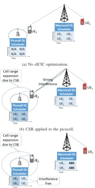
User off-loading and inter-cell interference management are not decoupled problems. The toy example in Fig. 1 illustrates the point that joint ABS and CSB optimization is needed to obtain good DL throughput performance, where the network consists of one macrocell, one picocell, and two users. Fig. 1a
shows the situation where eICIC is not applied, and both user equipment1 (UEs) will be attached to the macrocell even if UE2 is located near the picocell. In Fig. 1b, the picocell
modifies its CSB value so that UE2 is now attached to the
picocell even if the macrocell offers higher RSRP. In this case, UE1 can enjoy higher throughput because UE2 has been
off-loaded to the picocell. However, UE2 will suffer from low
throughput due to the strong interference from the macrocell. In Fig. 1c, the macrocell offers one of the two subframes (time slots) as an ABS and mutes its transmission on that subframe. Although UE1 enjoys less throughput in this case,
the throughput of UE2 can be greatly increased because it
is served by an interference-free subframe. Also, the total power consumption of the cells are greatly reduced while the users can achieve reasonably high data rate. By comparing the three cases in Fig. 1, we can see that joint ABS and CSB optimization can lead to a resource allocation pattern that strikes a good balance among fairness, high data rate, and energy efficiency.
Several algorithms of eICIC optimization exist in the lit-erature. Tall et al.’s algorithm in [3] performs optimization of ABS and CSB separately, where the ABS patterns are represented as fractional numbers. Deb et al. proposes a centralized algorithm that jointly optimizes ABS and CSB patterns in [4], where the interfering macrocells of a picocell are constrained to offer ABSs on the same subframes. In [5], Pang et al. propose a distributed algorithm that determines the number of ABSs without the optimization of CSB. Thakur et al. considered CSB optimization together with femtocell power control in [6]. In [7], Bedekar and Agrawal show that under certain simplifications, the joint optimization problem can be decoupled into optimizing ABS ratios and optimizing user attachment problems.
This paper aims at optimizing the proportional fair (PF) global utility of a LTE-A HetNet by using a distributed algo-rithm that jointly optimizes ABS and CSB patterns. Specifi-cally, we formulate an exact potential game, and we show that by randomly choosing a player and letting the player plays
(a) No eICIC optimization.
(b) CSB applied to the picocell.
(c) CSB applied to the picocell and ABS applied to the macrocell.
Fig. 1: Toy example of a LTE HetNet which consists of a macrocell, a picocell, and two users.
its best response will lead to a Nash equilibrium. Through simulation studies, we find out that our distributed joint ABS and CSB optimizer can improve the spectral efficiency by 20% and improve the energy efficiency by 46% while enhancing the fairness of the achieved user data rates. Also, we use different DL schedulers and compare their impact on various system performance indicators, and we find out that the scheduler based on convex relaxation can lead to 14% increase in spectral efficiency and 16% in energy efficiency compared to a conventional PF DL scheduler.
The rest of the paper is organized as follows. Section II gives the system model of the LTE-A HetNets. Section III formulates the joint ABS, CSB, and resource allocation optimization problem. Section IV proposes the distributed optimization algorithm based on exact potential game and describes three different DL schedulers. Section V presents
the numerical studies, and Section VI concludes the paper. II. SYSTEMMODEL
Consider a heterogeneous cellular network where picocells are deployed together with macrocells. Denote M and P as the set of macrocells and picocells, respectively. DenoteUi as
the set of users associated with station2 i, where i
∈ M ∪ P.
Let the vector γ denote the CSB values of all stations and let
γi denote the CSB value of station i, where each γi takes a
value in a pre-defined set of real numbersC. Let Pi
Rx,ube the RSRP of user u from station i, user u will be attached to the following station
g(u, γ), arg max i (P
i
Rx,u+ γi). (1)
Clearly, Pi
Rx,u depends on the transmission power of the serving station, the distance between the serving station and user u, the shadowing loss, and fast fading. These relevant parameters will be described later in the numerical studies section.
Suppose each station has the following resources, i.e., T equal-length subframes in the time domain and F equal-width resource blocks (RBs) in the frequency domain, where each subframe and RB pair forms a physical resource block (PRB). Denote B:= T · F as the total number of PRBs available at
each station. It is assumed that when a station is transmitting on a certain subframe, the transmission power allocated on all the PRBs is the same. Also, it is assumed that all PRBs are synchronized in both time and frequency domains.
Let αmbe the ABS pattern vector of macrocell m, where
the vector consists of T binary entries, and the values 0 and 1 indicate that the corresponding subframe is an ABS and a non-ABS, respectively. Let ru,b be the throughput of user u at PRB b, where b ∈ [1, B]. The actual value of ru,b is
affected by αm when macrocell m is either interfering or
serving user u. When user u is associated with macrocell m, its signal-to-noise-plus-interference ratio (SINR) on PRB b is then calculated as:
SINRmu,b= h m u,b· PRx,um · αm,τ(b) PInt,u,bM\{m}+ PP Int,u,b+ N0 ,
where hmu,b is the fast fading link gain on PRB b from macrocell m to user u, τ(b) returns the subframe index with
respect to PRB b, PInt,bM\{m}gives the interference power from macrocells inM \ {m} at PRB b, PInt,bP gives the interference power from picocells in P at PRB b, and N0 denotes the
additive white Gaussian noise (AWGN). When user u is served by picocell p, its SINR at PRB b is given by:
SINRpu,b= h p u,b· P p Rx,u PInt,u,bM + PInt,u,bP\{p}+ N0 ,
where hpu,bis the fast fading link gain from picocell p to user u at PRB b, PInt,u,bM gives the interference power from macrocells inM and PInt,uP\{p}gives the interference power from picocells
TABLE I: Descriptions of notations
Notation Description
αm ABS pattern of macrocell m
γ Vector specifying CSB patterns of all stations τ(b) The index of subframe of PRB (b)
g(u, γ) The station user u is associated with
hi
u,b Fading gain from station i to user u at PRB b
ru,b Throughput of user u at PRB b, where the serving station of the user is implicitly given
wu Weighting factor of UE u
xu,b Indicator of whether user u occupies PRB b of the serving cell
B Number of PRBs
F Number of RBs
N0 Noise power of a frequency subcarrier at a user
T Number of subframes
W Bandwidth per RB
A Set of vectors from which macrocells can choose ABS pattern
C Set of CSB values any station can choose from
M Set of all macrocells
P Set of all picocells
U Set of all users in the system
Ui Users associated with station i
in P \ p. It is assumed that the serving station knows the throughput of user u at PRB b, and the throughput can be calculated using Shannon’s capacity formula, i.e.,
ru,b= (
W· log2(1 + SINRm
u,b), g(u, γ) = m, W· log2(1 + SINRpu,b), g(u, γ) = p,
where W is the bandwidth of a PRB. Note that the interference power from the interfering macrocells depends on their ABS patterns. Table I summaries the notations used throughout the paper.
III. PROBLEMFORMULATION
We now present the resource allocation problem, where the ABS and CSB patterns of the stations are the main parameters to be optimized.
Let xu,b be the binary variable which tells if PRB b is
allocated to user u by its serving station, where xu,b = 1
indicates that user u occupies the b-th PRB and xu,b = 0
indicates otherwise. Assume a nonnegative weighting factor
wu is applied to user u. To achieve a good trade-off between
maximizing total throughput and user fairness, we aim to solve the following MAXPFUTILITY optimization problem:
maximize Pi∈M∪PPu∈U
iwu· ln PB b=1xu,b· ru,b, (2) subject to Pu∈U mxu,b= αm,τ(b), ∀m ∈ M, b∈ [1, B], αm∈ A, (3) P u∈Upxu,b= 1, ∀p ∈ P, b ∈ [1, B], (4) xu,b∈ {0, 1}, ∀u ∈ U, b ∈ [1, B], (5) γ(i)∈ C, ∀i ∈ M ∪ P, (6)
where the objective function is chosen to be the sum of log of users’ throughput so that proportional fairness among the users is the goal [8]. In the constraint (3), A denotes the set of ABS patterns that a macrocell can adopt.
We will discuss in more detail that MAXPFUTILITYis hard to solve in the next section. Also, a distributed algorithm based on exact potential game will be provided.
IV. DISTRIBUTEDALGORITHMUSINGGAMETHEORY
In this section, we describe the distributed algorithm based on exact potential game and various downlink schedulers. A similar approach for distributed optimization on power control and user association has been discussed in [9].
A. Exact Potential Game Formulation
In an exact potential game, there exists a potential function such that the change of the potential function due to the change of a player’s strategy is equal to the change of the payoff function of that player due to the change of its strategy. If players take turns randomly to update their strategies so that their payoff functions are maximized (i.e., best response), then the strategies of players will converge to a Nash equilibrium within finite steps of game plays [10], where the underlying assumption is that the game is finite.
Recall that our objective is to maximize the PF objective function in a LTE-A HetNet as stated in MAXPFUTILITY. When a station changes its CSB value or ABS pattern (in case of a macrocell only), the neighboring stations’ user attachment and DL throughput can be affected. Let the stations be the players. If each player’s payoff function takes the neighboring stations’ utilities into account, then the change of the global utility due to the change of a player’s strategy will be equal to the change of the payoff function of that player. This gives the intuition of how we can formulate the exact potential game.
Besides ABS and CSB patterns, the selection of DL sched-ulers also impacts the DL throughput of a station. In this paper, instead of including various schedulers in the strategy set of each station, we fix the selection of DL schedulers during game plays and compare system performance when different schedulers are used. We will describe the DL schedulers after formulating the exact potential game.
LetM ∪ P be the set of players. For joint ABS and CSB optimization, define the set of strategies that player i can adopt as
Si:= (
A × C, i ∈ M, C, i ∈ P,
so that macrocells offer ABSs and can adjust CSB values while picocells only adjust CSB values and offer no ABS. In the sequel we use player and station interchangeably. Denote s and si as the strategies played by all players and the strategy
played by player i, respectively. Let
s−i, (s1, ..., si−1, si+1, ..., s|M|+|P|),
be the strategies adopted by every player other than player i. Denote
(s′i, s−i), (s1, ..., si−1, s′i, si+1, ..., s|M|+|P|)
as the strategies of all players so that player i chooses strategy
Define the neighboring set of player i asNi, {i} ∪ NiInt∪ NAtt
i , where i ∈ M ∪ P, NiInt denotes the set of stations
whose downlink transmissions can be interfered by station i,
NAtt
i is the set of stations whose user attachment patterns can
be changed by modifying the CSB value of station i. Let the utility of station i∈ M ∪ P be Ui(s), X u∈Ui wu· ln B X b=1 xu,b· ru,b, (7)
where xu,b is given by the underlying scheduling scheme and
satisfies the constraints (3), (4) and (5). The total utility of all players is
U(s) = X
i∈M∪P
Ui(s). (8)
Let the payoff function of player i be
Vi(s), X j∈Ni
Uj(s).
We show that the function U(·) is a potential function in the
following theorem.
Theorem 1. The function U(·) is a potential function of the
game (M ∪ P, (Si, i∈ M ∪ P), (Vi, i∈ M ∪ P)).
Proof. Suppose we change the strategies of players from s to
(s′
i, s−i), then the change on U (·) is given as follows: U(s′ i, s−i)− U(s) = Pj∈M∪PUj(s′i, s−i)− Uj(s) = Pj∈Ni(Uj(s′i, s−i)− Uj(s)) + P j∈M∪P\Ni(Uj(s ′ i, s−i)− Uj(s)) = Pj∈Ni(Uj(s ′ i, s−i)− Uj(s)) (9) = Vi((s′i, s−i))− Vi(s), (10)
where (9) follows since the change of player i’s strategy only affects the utilities of players inNi, and (10) follows from the
definition of the payoff function of a player. Eqn. (10) indicates that the change of U(·) due to the change of the strategy of
a player is equal to the change of the payoff function of that player. Therefore, U(·) is a potential function of the game (M ∪ P, (Si, i∈ M ∪ P), (Vi, i∈ M ∪ P)).
Since randomly updating players’ strategies will lead to a Nash equilibrium if each player plays its best response, the procedure of the distributed optimization can be carried out as follows:
1) Initialize the ABS and CSB patterns of all macrocells. Initialize the CSB values of all picocells.
2) Select a player i randomly from M ∪ P. The player then tests all strategies in Si and selects the one that
maximizes Vi.
3) Repeat step 2 until some stopping criterion is met. Note that the same potential game framework can be used to optimize other objective functions. For example one may aim at maximizing the weighted sum of DL throughput of all users
[11], in this case it will be more reasonable to define the payoff function of a player in (7) asPu∈U
iwu·
PB
b=1xu,b· ru,b.
Moreover, the potential game framework can be used to per-form optimizations when only ABS patterns of the macrocells or only CSB values of the stations are allowed to be changed. For solely ABS optimization of macrocells, the strategy sets of all macrocells becomesA and the only strategy that a picocell has is to use all subframes and set its CSB value to 0 dB. For solely CSB optimization, the strategy set of each station isC. B. DL Schedulers
In this paper, we compare the performance of the distributed optimization algorithm using three DL schedulers.
1) Round-Robin (RR) Scheduler: A station simply allocates its PRBs to the attached users in turns. For example, suppose a station has five PRBs labeled as PRB1, PRB2, ..., and PRB5,
and there are two users attached to the station, then PRB1,
PRB3, and PRB5 will be allocated to user 1 while PRB2 and
PRB4 will be allocated to user 2.
2) PF Scheduler [12]: For station i, the b-th PRB at subframe t, given that the subframe is not an ABS, will be allocated to the following user
b ub , arg max u∈Ui ru,b ru(τ (b)) ,
where b ∈ [1, B], ru(t) is the long-term average throughput
of user u in subframe τ(b) and it is calculated as
ru(τ (b)) = (1−t1 c)ru(τ (b)− 1) +1 tcΣ{b′|τ (b′)=τ (b)}ru,b′· I{bu ′ b = u}.
In the above equation, tc is the time window to be chosen
and I{·} is the indicator function. The performance of this scheduler has been studied in several scenarios, see [13].
3) Convex PF Scheduler: Given a strategy, we wish to maximize the payoff function of a player as defined in (7) subject to the constraints (3), (4) and (5). This problem, however, has been proved to be an NP-hard problem in [14, Theorem 2].
On the other hand, if we take a picocell as an example, relax the integer constraint in (5) and formulate the following RELAXEDSCHEDULER problem
maximize X u∈Up wu· ln B X b=1 xu,b· ru,b, (cf. 7) subject to X u∈Up xu,b= 1, ∀p ∈ P, b ∈ [1, B], 0≤ xu,b≤ 1, ∀u ∈ Up, p∈ P, b ∈ [1, B], (11)
we have the following observations:
(a) The objective function is concave. To see this, note that lnPBb=1xu,b· ru,b is a composition of a concave
function and a linear function so that it is concave, and the objective function is therefore concave since it is a nonnegative summation of concave functions [15]. (b) The constraints are linear.
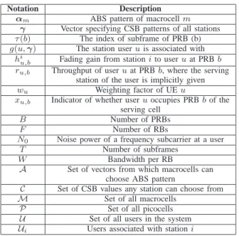
−3000 −2000 −1000 0 1000 2000 3000 −3000 −2000 −1000 0 1000 2000 3000
x−axis coordinate in meters
y−axis coordinate in meters
Fig. 2: A randomly generated hexagonal HetNet layout. The triangles, dots, and crosses represent macrocells, picocells and users, respectively.
As a result, we can solve RELAXEDSCHEDULERby changing the objective to minimizing the negative of (7) and use standard convex optimization solvers. Let xRelaxed
u,b be the
solution to RELAXEDSCHEDULER. To get a feasible solution of MAXPFUTILITY, we need to quantize xRelaxed
u,b so that the
constraints in (3), (4), and (5) are satisfied. The quantization can be done as xu,b:= 1, u = arg max u′ {x Relaxed u′,b }, 0, ∀u 6= arg max
u′ {x
Relaxed
u′,b },
where a tie is broken randomly in case arg maxu′{xRelaxedu′,b }
returns multiple answers for a given b.
The case when the station is a macrocell is similar except no user is assigned to the PRBs that are offered as ABSs. The details are omitted for simplicity.
V. SIMULATIONRESULTS
A randomly generated hexagonal HetNet layout is shown in Fig. 2, where the whole network consists of seven clusters of macrocells and the borders of each cluster are marked with bolded lines. Macrocells are located at the center of their respective hexagons. One picocell is placed within each hexagon in the center cluster, where the angle of the vector which starts from the hexagon center and ends at the picocell is randomly chosen and the distance from the picocell to the center of the hexagon follows triangular distribution. This will create an effect that the picocells are more likely to be located near the edge of each hexagon, an area where all neighboring macrocells impose strong interference. Also, for each hexagon in the center cluster, six users are placed within 120 meters from each picocell and another four users are placed within the hexagon. The distribution of the distances from the six
Fig. 3: ABS patterns that can be chosen by a macrocell. TABLE II: Parameters for Generating HetNet Topologies
Parameter Value
Inter-macrocell distance 1000 m
Minimum distance from macro to user 35 m Minimum distance from pico to user 10 m Minimum distance from macro to pico 75 m
Antenna per site Omnidirectional× 1
Macrocell power 40 W
Picocell Power 1 W
Noise density -174 dBm/Hz
Noise figure 9 dB
Duration per subframe 1 ms
Bandwidth per RB 180 kHz
CSB values {0, 3, 6, 9, 12, 15} dB
Log-normal shadowing 10 dB
standard deviation
Path loss from macrocell to user 128.1 + 37.6 log10d, d in km Path loss from picocell to user 140.7 + 36.7 log10d, d in km
users who are intentionally placed within 120 meters of a picocell follows triangular distribution, and the directions from the picocell to the six users are random. The other four users are similarly generated except the reference point becomes the respective macrocell. The six clusters surrounding the center cluster are exact copies of the center cluster. Other parameters are given in Table II.
The setup of the potential game is given as follows. The elements in M and P are the macrocells and the picocells in the center cluster, respectively. The weighting factors of all users are the same, i.e., wu= 1 for all u. T and F are set to
be 10 and 3, respectively. All possible ABS patterns are shown in Fig. 3, and all possible CSB values are given in Table II.
It is assumed that the users are static and the buffers of the stations are always fully loaded. Also, each PRB experiences independent Rayleigh fading with variance 1. The shadowing from a station to a user is calculated by adding a common shadowing value and a randomly generated shadowing value and then dividing the sum by √2, so that the shadowing
values are correlated [16]. The following results are obtained by averaging 200 randomly generated HetNet topologies.
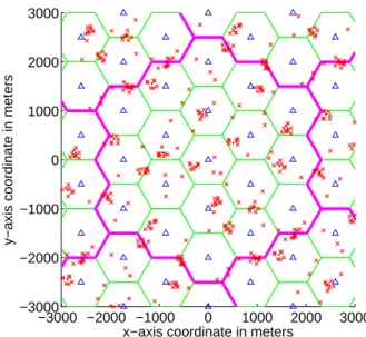
Fig. 4 plots the global utility functions as the potential games are being played, where the global utility function is defined in (8). The maximum number of iteration is set to be 300. We can see that all global utility functions increase as more iterations are played. Also, the global utility functions when the convex PF schedulers as described in Section IV-B3 are used are always larger than the global utility functions when the PF schedulers as described in Section IV-B2 are
0 50 100 150 200 250 300 1200 1250 1300 1350 1400 1450 1500 1550 Iteration
Averaged Global Utility
ABS+CSB, PF convex CSB, PF convex ABS, PF convex ABS+CSB, PF t c=40 ABS+CSB, PF t c=20 ABS+CSB, PF t c=5 CSB, PF t c=40 CSB, PF t c=20 ABS, PF t c=40 CSB, PF t c=5 ABS, PF t c=20 ABS, PF t c=5 ABS+CSB, RR CSB, RR ABS, RR
Fig. 4: Average global utility as a function of number of game plays.
used, and the global utility functions when the PF schedulers are used are always larger than the global utility functions when the RR schedulers are used. On average, a global utility function when the convex PF scheduler is used is about 5% larger than a global utility function when the PF scheduler is used, and a global utility function when the PF scheduler is used is about 15% larger than a global utility function when the RR scheduler is used. Three different values of the time window tc of the PF scheduler are tested, and the variation
of the global utility function due to different tc settings is not
large.
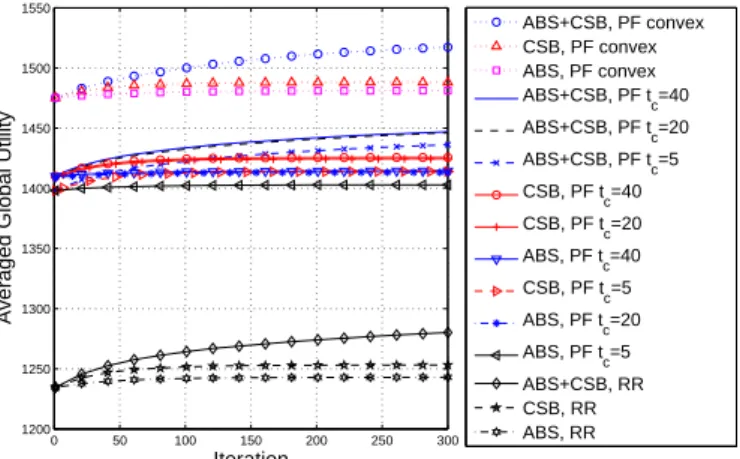
Fig. 5, Fig. 6, and Fig. 7 show the cumulative distribution functions (CDFs) of the achieved user rates when ABS to-gether with CSB optimization, ABS optimization, and CSB optimization are performed, respectively. The achieved rate of a user is defined as the sum of the per-bandwidth Shannon capacity of each PRB that is assigned to that user. We can observe from Fig. 5 that the user rates when joint ABS and CSB optimizations are performed are improved compared to the counterparts when no optimization is done. The user rates improvements due to ABS optimization and CSB optimization, as depicted in Fig. 6 and Fig. 7, respectively, are unfortunately not very obvious.
Fig. 8 gives the CDFs of the achieved rates of the worst 5% users of all randomly generated HetNets, where the convex PF scheduler is used in each of the four scenarios. We can see that the joint ABS and CSB optimization can help the worst users to increase their achieved rates.
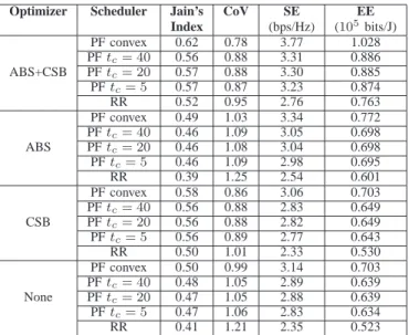
Table III summaries several performance indicators of dif-ferent game plays, where Jain’s Index stands for the Jain’s fairness index of the achieved user rates, CoV stands for the coefficient of variation on the achieved user rates, SE stands for the spectral efficiency defined as the average per-bandwidth capacity of all allocated PRB from cells in M and P, and EE stands for energy efficiency defined as the number of bits transmitted in all allocated PRBs from cells in M and P divided by the transmission energy used by all cells in M
0 10 20 30 40 50 60 70 80 0 0.1 0.2 0.3 0.4 0.5 0.6 0.7 0.8 0.9 1 User rate (bps/Hz) CDF RR RR, ABS+CSB PF t c=40 PF convex PF t c=40, ABS+CSB PF convex, ABS+CSB
Fig. 5: Comparison of CDFs of user rates when ABS and CSB are jointly optimized against the cases when no optimization is performed. For example, “RR” represent the CDF of user rates when no optimization is done and the scheduler is RR, “RR, ABS+CSB” represent the CDF of user rates when ABS and CSB joint optimization is performed and the scheduler is RR. 0 10 20 30 40 50 60 70 80 90 0 0.1 0.2 0.3 0.4 0.5 0.6 0.7 0.8 0.9 1 User rate (bps/Hz) CDF RR RR, ABS PF t c=40 PF t c=40, ABS PF convex PF convex, ABS
Fig. 6: Comparison of CDFs of user rates when ABS is op-timized against the cases when no optimization is performed. For example, “RR” represent the CDF of user rates when no optimization is done and the scheduler is RR, “RR, ABS” represent the CDF of user rates when ABS optimization is performed and the scheduler is RR.
0 10 20 30 40 50 60 70 80 0 0.1 0.2 0.3 0.4 0.5 0.6 0.7 0.8 0.9 1 User rate (bps/Hz) CDF RR RR, CSB PF t c=40 PF t c=40, CSB PF convex PF convex, CSB
Fig. 7: Comparison of CDFs of user rates when CSB is op-timized against the cases when no optimization is performed. For example, “RR” represent the CDF of user rates when no optimization is done and the scheduler is RR, “RR, CSB” represent the CDF of user rates when CSB optimization is performed and the scheduler is RR.
0 1 2 3 4 5 0 0.1 0.2 0.3 0.4 0.5 0.6 0.7 0.8 0.9 1
Achieved user rates (bps/Hz)
CDF
PF Convex, ABS+CSB PF Convex, CSB PF Convex, ABS PF Convex, no opti.
Fig. 8: The CDF of the worst 5% users’ rates.
and P. In general, we can observe that ABS and CSB joint optimization can lead to better user fairness, less deviation of user rates, higher spectral efficiency and higher energy efficiency. Specifically, if we compare the case when joint ABS and CSB optimization is performed and the case when no optimization is carried out while the underlying schedulers in both cases are the convex PF schedulers, then we can observe a 20% increase in spectral efficiency, a 46% increase in energy efficiency, and a larger fairness index achieved by joint ABS and CSB optimization. Also, if we compare the convex PF scheduler and the PF scheduler with tc = 40 when joint
ABS and CSB optimization is performed, we can observe 14% increase in spectral efficiency, a 16% increase in energy
efficiency, and a larger fairness index achieved by the convex PF scheduler.
TABLE III: Performance Indicators Optimizer Scheduler Jain’s CoV SE EE
Index (bps/Hz) (105 bits/J) ABS+CSB PF convex 0.62 0.78 3.77 1.028 PF tc= 40 0.56 0.88 3.31 0.886 PF tc= 20 0.57 0.88 3.30 0.885 PF tc= 5 0.57 0.87 3.23 0.874 RR 0.52 0.95 2.76 0.763 ABS PF convex 0.49 1.03 3.34 0.772 PF tc= 40 0.46 1.09 3.05 0.698 PF tc= 20 0.46 1.08 3.04 0.698 PF tc= 5 0.46 1.09 2.98 0.695 RR 0.39 1.25 2.54 0.601 CSB PF convex 0.58 0.86 3.06 0.703 PF tc= 40 0.56 0.88 2.83 0.649 PF tc= 20 0.56 0.88 2.82 0.649 PF tc= 5 0.56 0.89 2.77 0.643 RR 0.50 1.01 2.33 0.530 None PF convex 0.50 0.99 3.14 0.703 PF tc= 40 0.48 1.05 2.89 0.639 PF tc= 20 0.47 1.05 2.88 0.639 PF tc= 5 0.47 1.06 2.83 0.634 RR 0.41 1.21 2.35 0.523 VI. CONCLUSION
We have proposed a distributed game-theoretic-based al-gorithm for jointly optimizing the ABS and CSB patterns in LTE-A HetNets. Based on the potential game framework, we have demonstrated the necessity of jointly optimizing the ABS and CSB patterns, as simulation results suggest that large improvements on spectral efficiency, energy efficiency, and user fairness can be achieved by doing so. Moreover, we have compared two DL PF schedulers and showed that the scheduler obtained from relaxing an NP-hard resource allocation problem outperforms the other more conventional scheduler in terms of user fairness, spectral efficiency, and energy efficiency.
ACKNOWLEDGEMENT
This work was supported by ANR project IDEFIX under grant number ANR-13-INFR-0006 and in part by a grant from the Research Grants Council of the Hong Kong Special Administrative Region, China, under Project CityU 121713. A part of the work was carried out at LINCS (www.lincs.fr).
REFERENCES
[1] Cisco, “Cisco visual networking index: Forecast and methodology, 2013-2018,” June 2014.
[2] J. Andrews, “Seven ways that HetNets are a cellular paradigm shift,”
IEEE Communications Magazine, vol. 51, no. 3, pp. 136–144, March
2013.
[3] A. Tall, Z. Altman, and E. Altman, “Self organizing strategies for enhanced ICIC (eICIC),” CoRR, vol. abs/1401.2369, 2014. [Online]. Available: http://arxiv.org/abs/1401.2369
[4] S. Deb, P. Monogioudis, J. Miernik, and J. Seymour, “Algorithms for enhanced inter-cell interference coordination (eICIC) in LTE HetNets,”
IEEE/ACM Transactions on Networking, vol. 22, no. 1, pp. 137–150,
[5] J. Pang, J. Wang, D. Wang, G. Shen, Q. Jiang, and J. Liu, “Optimized time-domain resource partitioning for enhanced inter-cell interference coordination in heterogeneous networks,” in Proc. IEEE Wireless
Com-munications and Networking Conference (WCNC), April 2012, pp.
1613–1617.
[6] R. Thakur, A. Sengupta, and C. Siva Ram Murthy, “Improving capacity and energy efficiency of femtocell based cellular network through cell biasing,” in Proc. 11th International Symposium on Modeling
Optimiza-tion in Mobile, Ad Hoc Wireless Networks (WiOpt), May 2013, pp. 436–
443.
[7] A. Bedekar and R. Agrawal, “Optimal muting and load balancing for eICIC,” in Proc. 11th International Symposium on Modeling
Optimiza-tion in Mobile, Ad Hoc Wireless Networks (WiOpt), May 2013, pp. 280–
287.
[8] I.-H. Hou and C. S. Chen, “Self-organized resource allocation in LTE systems with weighted proportional fairness,” in IEEE International
Conference on Communications (ICC), 2012, pp. 5348–5353.
[9] C. Singh and C. S. Chen, “Distributed downlink resource allocation in cellular networks through spatial adaptive play,” in Proc. 25th
International Teletraffic Congress (ITC), 2013.
[10] J. O. Neel, “Analysis and Design of Cognitive Radio Networks and Dis-tributed Radio Resource Management Algorithms,” Ph.D. dissertation, Virginia Polytechnic Institute and State University, Sep 2006. [11] C. S. Chen, K. W. Shum, and C. W. Sung, “Round-robin power control
for the weighted sum rate maximisation of wireless networks over mul-tiple interfering links,” European Transactions on Telecommunications, vol. 22, no. 8, pp. 458–470, 2011.
[12] S. Sesia, I. Toufik, and M. Baker, LTE - The UMTS Long Term Evolution:
From Theory to Practice. Wiley, 2009.
[13] G. Caire, R. Muller, and R. Knopp, “Hard fairness versus proportional fairness in wireless communications: The single-cell case,” IEEE
Trans-actions on Information Theory, vol. 53, no. 4, pp. 1366–1385, April
2007.
[14] C. W. Sung, K. Shum, and C. Y. Ng, “Fair resource allocation for the gaussian broadcast channel with ISI,” IEEE Transactions on
Communi-cations, vol. 57, no. 5, pp. 1381–1389, May 2009.
[15] S. Boyd and L. Vandenberghe, Convex Optimization. New York, NY, USA: Cambridge University Press, 2004.
[16] GreenTouch, “Mobile communications WG architecture doc2: Reference scenarios,” May 2013.