HAL Id: tel-02895332
https://pastel.archives-ouvertes.fr/tel-02895332
Submitted on 9 Jul 2020HAL is a multi-disciplinary open access archive for the deposit and dissemination of sci-entific research documents, whether they are pub-lished or not. The documents may come from teaching and research institutions in France or abroad, or from public or private research centers.
L’archive ouverte pluridisciplinaire HAL, est destinée au dépôt et à la diffusion de documents scientifiques de niveau recherche, publiés ou non, émanant des établissements d’enseignement et de recherche français ou étrangers, des laboratoires publics ou privés.
along a 1000 m elevation gradient in the French
Southern Alps
Seyedehmasoumeh Saderi
To cite this version:
Seyedehmasoumeh Saderi. Wood formation dynamics of Larch (Larix decidua Mill.) along a 1000 m elevation gradient in the French Southern Alps. Silviculture, forestry. AgroParisTech, 2017. English. �NNT : 2017AGPT0015�. �tel-02895332�
N°: 2017AGPT0015
Doctorat AgroParisTech
T H È S E
pour obtenir le grade de docteur délivré par
L’Institut des Sciences et Industries
du Vivant et de l’Environnement
(AgroParisTech)
Spécialité : Sciences du bois et des fibres
présentée et soutenue publiquement par
Seyedehmasoumeh SADERI
Le 21 Décembre 2017Dynamiques de la formation du bois du Mélèze
(Larix decidua Mill.) le long d’un gradient
altitudinal de 1000 m dans les Alpes du sud Françaises
Directeur de thèse : Mériem Fournier Co-encadrement de la thèse : Cyrille Rathgeber
Jury
M. Philippe Rozenberg, Directeur de recherche, INRA Rapporteur, Président
M. Kambiz Pourtahmasi, Professeur, Université de Téhéran, IRAN Rapporteur
Mme. Marina Bryukhanova, Senior researcher, Russian science Academy, Russie Examinatrice
Mme. Mériem Fournier, Chargé de recherche, INRA, Nancy Directeurde thèse
M. Cyrille Rathgeber, Chargé de recherche, INRA, Nancy Co-directeur de thèse
AgroParisTech UMR INRA AgroparisTech
Firstly i would like to express my sincere gratitude to my supervisors Mériem Fournier for her help, support and guidance along this thesis.
Secondly from Cyrille Rathgeber for his support and insightful comments and en-couragement during my thesis that incentented me to widen my research from var-ious perspectives.
I would like to express my sincere gratefulness to the all people from LERFOB and INRA who helped me during this thesis. Specially from those helped in the field work: Emmanuel Cornu, Pierre Gelhaye, Alain Mercanti, Etienne Farré, Charline Freyburger, Natasha Clairet, Ignacio Barbeito.
I want to express my special thanks from Maryline Harroué for her help in anatomi-cal slides preparation and from Julien Ruelle who was always available for technianatomi-cal supports.
I want to express also my gratitude also from my colleagues at INRA, Nathalie Morel, Elodie Taillefumier, Thiéry Constant, Gérard Nepveu, Jana Dlouha and Francis Colin and all my friends and phd students at INRA and Agroparistech.
I would like to thank from the people in Agroparistech Michele Besancon, Corine Martin and also Christiene Fivet in phd school for their patience and help.
I want to thank also from Kambiz pourtahmasi from university of Tehran, who taught me the alphabet of wood science.
I would like to thank my family and specially my parents for the whole things they did in my the life. Their help and support even from long distance always made me motivated to do this thesis.
And finally i am eternally grateful from my dear husband Abedin Ferdousi for his constant love, patience and support during my life and specially this thesis.
1 General Introduction 7
1.1 Importance of wood formation studies . . . 8
1.2 Wood formation monitoring . . . 16
1.3 Characteristics of selected species, European Larch . . . 17
1.4 General context of study . . . 19
1.5 Objective and plan of the thesis . . . 22
2 Material and methods 29 2.1 Geographical location of study site . . . 30
2.2 Characteristics of selected trees . . . 31
2.3 Environmental variables . . . 33
2.4 Measuring the stem diameter changes in trees . . . 41
2.5 Wood formation variables . . . 46
3 Wood formation monitoring 71 3.1 Introduction . . . 73
3.2 Material and methods . . . 75
3.3 Results . . . 79
3.4 Discussion . . . 83
4 Wood formation phenology 95 4.1 Introduction . . . 97
4.2 Materials and methods . . . 99
4.3 Results . . . 102
4.4 Discussion . . . 113
5 Wood formation dynamics 125
5.1 Introduction . . . 127
5.2 Materials and methods . . . 129
5.3 Results . . . 133
5.4 Discussion . . . 141
5.5 Conclusion . . . 143
1.1 Structure of tree stem layers.. . . 10
1.2 Xylem structure in conifers. . . 10
1.3 Tracheid structure in conifers. . . 11
1.4 Schematic cross-sections of wood . . . 14
1.5 Cell wall layers. . . 15
1.6 Distribution of Larch.. . . 18
2.1 Map of study site in Briançon . . . 30
2.2 Photo of study site. . . 31
2.3 Schematic view of study site.. . . 31
2.4 Comparison of age, diameter and height of trees . . . 32
2.5 Monthly mean temperature (Storm) . . . 34
2.6 Comparison the annual mean temperature . . . 34
2.7 Mean temperature at tree stem . . . 35
2.8 Comparison the temperature (Storm via dendrometers) . . . 36
2.9 Comparison temperature of Meteo France stations . . . 37
2.10 Comparison meteo data from Storm and Meteofrance . . . 38
2.11 Long term comparison of temperature and rain . . . 39
2.12 Comparison of GDD . . . 40
2.13 Comparison of precipitation . . . 41
2.14 Comparison of air humidity . . . 42
2.15 Photo of manual band dendrometer . . . 43
2.16 Mean stem size increment by dendrometer . . . 44
2.17 Stem increment . . . 46
2.18 Trephor . . . 47
2.19 Marking microcore . . . 49
2.20 Impregnation machine . . . 49
2.22 Rotary microtom . . . 50
2.23 Cuting sample by microtom . . . 50
2.24 Coloration of the samples . . . 51
2.25 Developing radial xylem file in conifers . . . 53
2.26 Transverse section of a tracheid . . . 55
2.27 Comparison of radial wall thickness . . . 55
2.28 Comparison the lumen area . . . 56
2.29 Developement of traumatic resin canal . . . 57
3.1 Callus tissue in larch . . . 77
3.2 Growth curves. . . 77
3.3 Traumatic resin canal . . . 79
3.4 Number of resin canals . . . 80
3.5 Quantification of problem by regression analysis . . . 81
3.6 Cell number variation. . . 81
3.7 Regression of cambial stimulation . . . 82
3.8 Residual analysis . . . 83
4.1 long term climatic data comparison. . . 103
4.2 Climatic data Briancon. . . 104
4.3 Comparison of meteo data along gradient . . . 105
4.4 Wood formation phenology and duration. . . 107
4.5 Comparison of age and diameter. . . 109
4.6 Comparison of temperature at bE. . . 110
4.7 Comparison of temperature at cE. . . 111
4.8 Comparison of mean temperature at bE and cE. . . 112
4.9 Comparison of GDD at bE and cE. . . 112
4.10 Comparison of photoperiod at bE and cE. . . 113
5.1 Comparing growth dynamics parameters . . . 134
5.2 Duration of wood formation phases. . . 135
5.3 Gompertz function models. . . 137
5.4 Ring cell number regression . . . 138
5.5 Plot of sensitivity analysis . . . 139
5.6 Comparison of REW . . . 140
1.1
Importance of wood formation studies
1.1.1
The importance of wood
Wood is the most important natural and renewable source of energy and material. It has always had a crucial role in the history of human life. Nowadays it is still used as a privileged raw material in building, transport, furniture, art and sport.
The global production of round wood was reported 3714 million m3 in 2015 with
an increase of 19% compare to 1980 (FAO 2015). The rising demand for forest
products will continue with growing world population and income. The majority of wood (80%) can be find in forest that cover one third of the land area on the earth
(FAO 2010). Forests are considerable sources of food, energy and clean water for
living organisms. Forests contribute to a wide range of environmental services such as supporting sustainable agriculture, stabilizing soil and climate and production
of wooden and non-wooden materials(FAO 2016). The major planet’s biodiversity
depends on forest ecosystems. The broad variety in forest types including tropical, subtropical, mediterranean, temperate and boreal forests provide habitat, shelter and food for millions of plants, animals and insects species.
One of the most substantial roles of forests is participating in the carbon cycle, the backbone of life on the earth. Carbon is the fourth most abundant chemical element
in the universe (Ren et al. 2013). The food, civilization, economy and transport
system of human beings are based on carbon. Trees have the ability of sequestration of atmospheric carbon in their above and below-ground biomass structures through
photosynthesis(Unwin and Kriedemann 2000). Carbon dioxide is absorbed through
photosynthesis process by trees and convert into structural carbon in the form of cellulose, hemicellulose and lignin. The recent climatic changes highlighted the im-portance of carbon cycle in the last decades. Climate change has been defined as the statistically significant variation in the variables that define the climate of a region
or it’s variability persistent over an extended period of time (IPCC report 2014).
The effects of climatic change due to increasing atmospheric CO2 can be observed
as changing temperature and modifying precipitation regimes.
Because of the all mentioned functions provided by forests, they need to be stud-ied and protected. But disastrously, the extent of the world’s forests has declined substantially in the recent decades. In this situation, it is crucial to use and pre-serve wood resources much more efficiently. One of the solution to provide woody
resources is to grow wood using silvicultural plantations. In order to have a plan-tation with maximum economic yield we need to have a good understanding of the mechanisms involved in wood formation process in different tree species and also finding the optimum environmental condition for their growth.
1.1.2
Wood function in trees
Tree has been defined as a form that a plant develops to become one of the tallest, free standing and perennial plants. All the plants like trees need to face the problem of gravity. Tree stem must be strong enough to support the crown under the wide range of stresses such as storms. The 4000 years old Bristlecone pine, is an example of
a tree species that manage to survive against all the environmental stresses(Wilson
1984). Trees are able to cope with these problems through strengthening their stems
via wood formation.
The woody cells composed of cellulose and lignin, the two materials conferring the strength of wood, originally produced by the photosynthetic process in the leaves. Cellulose is the most abundant biological compound on the earth. The vascular cambium is composed of a thin layer of meristematic cells located between the secondary phloem (i.e., the living bark) and secondary xylem (i.e., wood). It is the responsible of making a continious envelope around the stems, branches and root of woody plants, producing xylem towards inside of the stem and the phloem outward
(Wilson 1984) (figure 1.1). The woody structure plays four essential functions in
trees: 1) supporting and distributing photosynthetic tissues; 2) transporting and uptaking the raw sap flow (nutrients and water) from the roots to leaves; 3) storing water and carbohydrates and other compounds; 4) storing and distributing defensive
compounds in order to protect the trees against pathogens(Kozlowski and Pallardy
1997, Fournier et al. 2006).
1.1.3
Tree ring structure in conifers
In the microscopic observation of the transverse section in conifers, tracheids, parenchyma, rays and resin canals can be observed (figure 1.2). The basic structure of a conifer tree ring from pith toward the bark consists of earlywood, transition zone and late-wood. The tracheids comprise 90 % or more of the total number of cells in conifers
Figure 1.1: Structure of tree stem layers
in trees. Tracheids are elongated, spindle shapes cells of 3−6 mm in the length and
6−60 µm in diameter (Sperry et al. 2006) that are closed at their end (figure 1.3).
The morphology of tracheids depends on the time in which they are produced within the growing season. The tracheids of early wood form at the beginning of growing
season and have larger lumen area and thinner cell wall compare to late wood
(Wil-son 1984). Tracheids are connected through openings in their secondary lignified
cell walls known as bordered pits (Carlquist 2013). The tracheid cells, die at the
end of their development to fulfill their function. The parenchyma cells are the only cell types that stay alive for a couple of years.
Figure 1.3: Structure of tracheid elements in conifers (Edited fromTaiz and Zeiger 2010).
1.1.4
Cambium definition and function in trees
Cambium is responsible of wood formation in trees. It has been defined as the sheath of dividing meristematic cells between the bark and wood, producing both new wood and bark. Meristems are groups of undifferentiated cells that retain the ability to
divide almost indefinitely (Wilson 1984). The origin of the word "cambium" was
found in the Arabic language, where it was used in medicine and surgery (Larson
1969). Malpighi 1678 had the original idea of defining cambium as responsible of
wood formation "the new layers of wood in stem and branches resulted from the
periodic transformation of the inner layers of the bark"(Sachs 1890).
Nehemiah Grew used firstly the term of cambium in a botanical sense in edition of
his book "The Anatomy of Plants" (Grew 1965). The formation of annual xylem
rings occurs due to the production of new cells by cambium division, the growth of cambial derivatives by expansion, and secondary wall thickening. The former two processes determine the annual increment width and the latter one the accumulation
of biomass in cell walls (Antonova and Stasova 1993). Trees also use the cambial
activity for thickening the roots to make the trees strong enough to overcome the
stresses of wind and gravity (Wilson 1984). Cambium is the main carbon sink in
trees participating in the carbon allocation via photosynthesis (Hansen and Back
1994).
Toward the end of summer, in temperate and boreal zones, the cambial activity slows down and the number of cells in the cambial zone returns to their minimum number in the dormant tree. Cambium of trees is bigger in area compare to other
plants because of their bigger size, making trees a good choice for studying cambial
activity(Wilson 1984).
Wood presents a variety of physical properties and chemical components. These properties are formed as the result of changes which took place during the differen-tiation process and conversion of cambium derivations into mature xylem elements
(Barnet 1981). The onset of wood formation is not directly detectable through bud
break or leaf phenology observation since it occurs in the inner part of the stems. Defining the dates of xylogenesis requires precise and direct measurement of cambial activity in a regular and short interval repetition along the growing season. Each cambial cell (the cambial initial), produces daughter cells to the inside and outside of the tree, along a radius of stem cross section. Derivations of cambial cells then go through the phases of enlarging, wall thickening and finally the programmed death of cells.
Cambial cell division
In the dormant season, the vascular cambium is inactive, and the cambial zone consisting in two to six layers of cells. These cells are rectangular in cross section, contain protoplasm in a viscous state and have clearly defined walls. The cambium cells are recognized by their thin primary walls, small radial size and rectangu-lar shape compare to phloem cells. The formation of a xylem cell can be divided into five main steps. 1) the periclinal division in a mother cell that produces a new daughter cell; 2) the enlargement of the newly formed cell; 3) the secondary cell wall formation that is the deposition of cellulose and hemi-cellulose in cell wall; 4) the im-pregnation of cell walls with lignin and 5) the programmed death of cells (figure 1.4).
Enlarging phase
Cell enlargement is the first stage of cell differentiation in plants. During this phase an irreversible increase occurs in the cell volume. The visible result of cell enlarge-ment is the great increase in the cell size that can multiplied the cell size by 10-100.
(Vaganov et al. 2006). This change in the cell size are the result of relaxation of
pri-mary cell wall in order to create a passive inlet of water which is counter balanced by an active influx of solutes. These steps are crucial to maintain a high turgor
pressure in the cells (Cosgrove 2005).
but turgor pressure can be considered as the engine of this phase. As a result
any water shortage with changing turgor pressure can affect cell growth
(Perrot-Rechenmann. 2010).
Secondary cell wall formation and lignification
The secondary wall which is the most important layer of cell is made of three main
elements that are cellulose, hemicellulose and lignin(Barnet 1981). The cellulose in
the secondary cell wall of tracheids and fibers is organised in three layers of S1, S2 and S3 from outside to inside of cell lumen which presents quite similar composition but different thickness and orientation of cellulose microfibrils (figure 1.5). The outer layer of (S1) has a crossed helical organization. It is the thinnest layer of secondary wall with 0.1 to 0,35 µm thickness.
The microfibril angle to the cell axis in this layer is 60◦ to 80◦. The (S2) layer has
a steeper helix than (S1) with a uniform helical organization. The thickness of this
layer is 1 to 10 µm and the microfibril angle is 5◦ to 30◦ to the cell axis. The third
internal layer of the secondary wall is (S3) that the structure of helix is similar to (S1). It is a thin layer with the thickness of 0.5 to 1,10 µm, with a microfibrils angle
of 60◦ to 90◦ (Barnett 1981, Plomion et al 2001).
After the end of cell enlargement, the secondary cell wall formation starts with the deposition of S1 layer between the membrance and the primary wall, soon followed by formation of S2 and S3. The secondary cell wall covers whole the surface except pit membrances. This phase is known to be controlled by the expression of genes that activate the transport, deposition and biosynthesis of wall components.
Lignification is a process whereby the stem becomes woody. During this phase a cell with a thin and viscoelastic walls converts to an anisodiametric cell with a
rigid and thick wall (Barnet 1981). Lignification begins at the corner of the cells in
the primary cell wall at the same time as S1 layer deposition then goes toward the middle lamella. In this step lignin deposit inside the spaces left by the microfibrils to make chemical bonds with hemicelluloses and act as a cement that make the cells water proof. The lignification process was reported to be sensitive to temperature. Although the hormonal control on the lignification process is not clear but the effect of ethylen in inducing several enzymes that are involved in the biosynthesis of lignin
Figure 1.4: [
Schematic cross-sections of the resting and developing radial xylem cell files in conifers.](A) Dormant cambium during winter composed of a thin band of 4–6 reinforced cambial cells layers, (B) Active cambium and associated developing radial cell files at the beginning of summer. The active cambium, composed of a
wide strip of 11–13 cambial cells layers, is located between the newly formed phloem and xylem. The developing xylem, which is composed of an enlarging zone
(3–4 cell layers), a thickening zone (7 cell layers), and a mature zone (12–13 cell layers), is located between the cambium and the previous tree ring. (C) Schematic view of a developing xylem radial file. Cell I represents a newly formed phloem cell of the current year. Cells II–IV shows cambial cells, of which cells III and IV are dividing. Cell V shows an enlarging cell. Cells VI–VII show thickening cells. Cell VIII shows a mature xylem cell (there is no cytoplasm in it). Cell IX represents a latewood cell of the previous tree ring. Green backgrounds represent cytoplasm, green lines represent cell membranes, blue lines represent cellulosic cell walls (dark
blue for primary walls, light blue for secondary walls), and red areas represent
lignified cell walls (Rathgeber et al. 2016).
Programmed cell death
Maturation is the last phase of wood formation. The xylem cells die to become func-tional and the only cell type that escape the death and stay alive for several years is
Figure 1.5: Microfibril orientation on the outer surface of primary wall and the secondary wall layers of S1, S2 and S3 of a conifer tracheid. CML shows the compound middle lamella. (Edited fromRafsanjani et al. 2014)
parenchyma. The principal trigger of this phase is a massive influx of calcium ions
(CA2+) to the vacuole through plasma membrance channels.
Then the vaccuole breaks up rapidly (in few minutes) as a sudden and the cyto-plasm is hydrolysed. After some days, the cell is formed as an empty space area with thick lignified wall with pits (Bollhoner et al. 2012). The mechanisms that control the death of cells were found to be connected to secondary wall formation. Programmed cell death is an essential step of xylem cell differentiation. It allows the mature xylem cells to perform their substantial function of mechanical support in the wood and conducting sap flows through their pits.
Cell cycle
Cell cycle, can be defined as the sequence of successive events that are highly con-trolled in all the cellular organisms that have nucleus. In the cell cycle, the meris-tematic mother cells undergo several developmental stages including division of the
nucleus and separation of cytoplasm in order to produce two daughter cells(Lachaud
et al. 1999). The cell division process in the cambium is slow and lasts about 10 to
50 days depending on different developmental stages, tree species and environmental
1.2
Wood formation monitoring
1.2.1
Importance of wood formation studies
Monitoring the seasonal dynamics of wood formation in trees started more than 50 years ago with the aim of better understanding the influence of climatic factors on trees growth, phenology of cambial activity and wood formation dynamics. With the recent climatic changes, this question grabbed more attention and led to in-crease in the number of studies in the last decades. In conifers the diameter and wall thickness of tracheids along a radial file are divided and multiplied by factor 5
respectively(Vaganov et al. 2006, Cuny et al. 2014). It shows the variation in wood
anatomy within a single tree ring. These transition depend on the species and the specific environmental condition along the wood formation period.
The aim of wood formation monitoring is finding to what extent these anatomi-cal changes are related to climatic constraints. Cambial activity is affected by the interaction between endogenous and exogenous factors. As described recently by
Cuny et al (2016), there are two main explanations to describe the tracheid cells
development in conifer tree rings. One is the developemental theory that relates the
tree ring formation mainly under the control of internal signals (Uggla et al 1996,
1998, Sundberg 2000, Oribe et al. 2003), according to that, the developemental
stages of tracheid cell formation is affected by the concentration of phytohormones
such as auxin (Uggla et al 1996). The second theory is the environmental theory
describing the anatomical changes within a tree ring to be under the control of
en-vironmental factors (Larson 1969, Fritts et al 1999, Vaganov et al 2011). A lot of
studies have been developed based on these two theories to understand the mecha-nisms that control the different response of cambial activity in different species and latitude/altitude.
Although the effect of environmental factors on the wood formation phenology(De
luis et al. 2007, Rossi et al. 2007, Gricar and Cufar 2008, Makinen et al. 2008, Gruber et al. 2009, Swidwark et al. 2011, Rossi et al. 2011, Balducci et al. 2013,
Ziaco et al. 2016), along elevation gradients (Moser et al. 2010, Treml et al. 2015,
Wang et al. 2015), maximum rate of cell production (Rossi et al. 2006), the
dy-namic of cell production (Rathgeber et al. 2011, Cuny et al. 2012) and its kinethic
(Cuny et al. 2014), have been studied widely but there is still lack of knowledge in
revealed that cambial activity is a complex dynamic system in trees. Without a clear understanding of the biological process that control each part of this system, it is not possible to define it’s response to different environmental conditions and specially extreme events such as low temperature.
1.2.2
Method of wood formation monitoring
As a classical model of wood formation monitoring, samples are extracted along the growing season from tree stems. In order to avoid disturbance to trees, wood samples are repeatedly extracted as small cores or so called microcores (Deslauriers et al. 2003). Generally, sampling is done after removing bark, by means of a small cutting tube hammered into the stem. Although microcoring is known as one of the less destructive methods of wood formation, it can induce the wounding responses
in trees. These reactions can be in the form of traumatic resin canals(Bollschweiler
et al. 2008, Schneuwly et al. 2009) or callus tissue formation (Stobbe et al. 2002).
Although microcoring method is widely used for wood formation studies but there is a gap to find the the effect of this method on the xylogenesis process and the final tree ring structure.
1.3
Characteristics of selected species,
Euro-pean Larch
1.3.1
Distribution of European Larch
Larch (Larix sp.) is a pioneer, very long-lived, fast-growing coniferous. It is one of the most abundant conifer species in the northern hemisphere. Larch belongs to
the Pinaceae family (Matras and Pâques 2008) and the genus includes 10 species
occurring in North America and Eurasia (Farjon 2010). It occurs naturally in the
Alps, at the border of Czech Republic and Poland (the Sudeten Mountains), North Slovakia and southeastern Poland (Western Carpathians) with some residual stands in Central Poland and Romanian carpathians (figure 1.6). The upper limit of Larch in the Western Alps is 2300 m while it’s lower limit can be observed at 1300 m
in the south-western part of the Alps (Wagner 2013). Larch has a large ecological
amplitude. In the Alps and Tatra Mountains it occurs in continental climates, with dry and very cold winters while in Poland and in the Sudeten Mountains it can grow
Figure 1.6: Distribution of Larch(Matras and Pâques 2008)
1.3.2
Characteristics of European Larch
European larch (Larix decidua Mill.) is one of the few deciduous conifer species. It’s small wind-dispersed pollen doesn’t have air sacs like the pollen of other conifers,
let them to move in less extensive dispersal up to 300 m by wind (Sjögren et al.
2010). They reach to sexual maturity at the age of 15 in open stands but at the age
of 35-40 years in close stands. They can produce valuable hybrids by crossing with
some other larch species such as Japanese larch (Larix kaempferi (Lamb.) (Matras
and Pâques 2008). This typical pioneer conifer is a light-demanding species with a
low competitive ability. Their close and enduring stands are established only when climatic conditions eliminate their competitors, such as mountain areas.
Larch can grow on a wide range of soil types, ranging from deep, well-structured and aerated to shallow stony soils, including calcareous soils, with a medium ground
water level(Wagner 2013). The age of larch trees under optimal conditions and free
standing can reach up to 600-850 years, while under forest conditions, their age will
continental alpine climates, it’s tolerance to very low temperature can be related to
the ability of losing needles and avoiding foliage desiccation (Wagner 2013).
1.3.3
Economically and ecological importance of French Alps
and European Larch
The Alps, known as one of the major mountain ranges in Europe, have a significant role in providing water cycle resources. It is called as "water tower of Europe". This notion points to the climate of Alps with abundant precipitation and snow falls. It has also an important role in sorting fresh water and moderating the variations in
river runoff(Isotta et al. 2014 ). But the occurrence of heavy precipitation and dry
periods, can be a threat for the components of the Alpine ecosystem.
French Alps have valuable species both ecologically and economically. Using larch in
historical building of ancient Rome was found by the archaeological studies(Matras
and Pâques 2008). It is one of the fastest-growing conifer species in Western and
central Europe and is planted even outside it’s natural range due to it’s silvicultural importance. The economical value of this species originates from both wood and resin production. It’s wood is characterized by a high density and durability making it a valuable raw material in building industry, pulp for paper and also furniture making. The essential oil of Larch is used also in aromatherapy. High concentration of tannins (up to 10%) and resin content (about 2.6%) increases the durability of
this species (Praciak et al. 2013). Under the optimal condition Larch can produce
more than 10 m3 of wood per ha annually (Matras and Pâques 2008).
1.4
General context of study
1.4.1
Phenology as a life trait in trees
In plants, phenology is the trade-off between the environmental factors and the
ac-cessablity of required resources for their growth(Nord and Lynch, 2009). Changing
temperature and precipitation pattern as a result of recent climatic changes are likely to drive significant modifications in all aspect of plants life such as
phenol-ogy, distribution, mortality and interactions with other organisms(IPCC 2014). In
temperate and boreal regions, this period shows the most favorable time for the tree-ring formation. It is the time window during which trees are open to receive the environmental signals and record them in the form of tree ring structures. Trees
growing in temperate regions experience short term environmental changes in dif-ferent season. They need to protect themselves to be able to survive in occurrence of freezing temperature. Going to dormancy is one way of doing that.
Timing of onset and cessation of wood formation are the two critical factors iden-tifying the limits of growing season period. Tree ring width at their range limits found to be mainly related to the growing season temperature. Bud break and leaf unfolding in adult trees are timed accurately to avoid the freezing damages. The range limits of tree species are set by the interaction between freezing resistance in spring and giving the enough time to the differentiation and autumnal maturation
of xylem cells (Korner 2016). So monitoring the phenology of wood formation in
trees growing in contrasting climate condition such as varying temperature reveals useful information about the response of tree species in a changing climate.
1.4.2
Elevation gradients in ecological studies
Elevation gradients provide useful natural experiments for ecological surveys because temperature, the main factor driving phenology of plants and animals decrease by increasing elevation. Mountain is defined as any elevation of land area from plains
that is 300 m above the sea level (Kapos et al. 2000). Moving toward higher
al-titudes, the environmental condition will change and the species need to be well adapted into the local condition in order to be survived. Mountains provide valu-able basis to test and develop the adaptation theories. In order to test the theories of species adaptation to elevation, it is crucial to understand the concept of elevation gradient to make the evaluation biological meaningful.
The global geophysiological change with altitude is decreasing land area and as a
result the opportunity for life(Korner 2000). Four main atmospheric changes found
to be associated with altitude. The first one is decreasing atmospheric pressure and
also partial pressure of all atmospheric gases such as O2 and CO2. These two gases
are the vital components of life and are related to the respiration in animals and gas exchange and photosynthesis in plants. Second is decreasing temperature by increasing altitude. Another global atmospheric change with increasing altitude is solar radiation that increases under a clear sky and the last is higher fraction of UV-B radiation. Precipitation and wind velocity although are not globally related
to altitude change(Korner 2007).
All the factors that are physically related to altitude can induce selective pressure
respond to the climatic changes in three basic ways: they persist in the modified
climate, they migrate to more suitable climates or they will be extinct (Guisan et
al. 1995). Their persistence can be in the form of phenotypic plasticity or gradual
genetic adaptation (Davis and Shaw 2001, Aitken et al. 2008).
Phenological characteristics show significant phenotypic variability along elevation gradients and presence of phenotypic variability is a sign of local adaptation. Moni-toring wood formation in trees is a way to assess the phenotypic response of trees to their environment. Different phases of wood formation (onset of cell enlargement, onset of cell wall thickening and the occurrence of the first mature cell) in larch were
found previously to be highly correlated to elevation(Moser et al. 2010).
Recent rapid climatic changes raise uncertainty about the ability of tree species to keep pace with their changing environment. In elevation gradients, there are cli-matic trend that are not generally related to elevation such as precipitation. But the pattern for precipitation (water and snow) in the Alps was found to increase
with increasing elevation due to local and regional effects(Sevruk 1998).
In addition to climate variables, there are other environmental factors that may not present altitudinal trend but may vary along elevation gradients and affect the phe-notypic response of species. These factors can be biotic or abiotic. The amount of relative extractable water for trees along elevation gradients can change dependent on the factors such as soil type or the amount of precipitation. So in elevation re-lated studies it is important to consider the environmental factors that can influence phenotypic variability in species.
The upper (northern) and lower (southern) limits of a species was found to be shaped generally by different ecological factors. The upper range of it’s distribution
was found to be temperature limited and the lower limits by water availability
(Sc-holes, 1994).
In this study European Larch trees (Larix decidua Mill.) growing along a gradient of 1000 m in elevation ranging from 1350 to 2300 m in French Alps were selected. Along this elevation gradient, trees are expected to experience contrasting climatic condition. The temperature variation is likely to affect the phenology of wood for-mation in trees growing in different elevations. Different precipitation regimes may have also an affect on their phenotypic responses. Monitoring wood formation along this gradient of 1000 m in elevation can help us to understand how trees are able to adjust their phenology and dynamics in order to adapt themselves to contrasting climate variables. In this way it is possible to find the optimum elevation for the growth of larch trees in Southern Alps and also to predict the response of this trees
to the main climatic changes such as temperature increase in future.
1.5
Objective and plan of the thesis
The main objective of this thesis is to study is to understand how trees are able to grow in contrasting climate conditions by adjusting cambium phenology, wood formation dynamics and resulting tree-ring width and structure.
After chapter one which is the general introduction, in chapter 2 the material and methods that have been used for this study are presented in details.
In chapter 3, the objective to check that classical wood formation moniroitng technics (e.g. weekly microcores sampling) do not influence xylogenesis, thus pro-ducing artifactual results such as wounding tissue or traumatic resin canals as de-fensive responses of studied trees was assessed.
The chapter 4 mainly focuses on the phenology of wood formation along the studied elevation gradient. The accurate timing of onset and cessation of cambial activity phases, as critical dates of cambial activity were extracted and compared in different sites. Then their trend along the gradient and relationship with the en-vironmental factors were described in the selected gradient using simple and mixed linear models and non-parametric bootstrap tests.
Chapter 5 is based the comparison of Larch cambial activity dynamics in the Larch trees along elevation gradient. wood growth dynamics was describe fitting Gompertz models and growth rate as well as cell cycle length and the number of dividing cambial cells were computed. The contribution of rate and duration of cambial activity in the production of the total annual ring cell number was evalu-ated using sensitivity analysis of a basic physical model.
Chapter 6 is the general discussion where the main findings from the previous chapters are presented. The aim of this chapter is to draw a comprehensive picture of the relationship between the obtained results from the wood formation monitoring along an elevation gradient in the French Alps as a response to the environmental factors for drawing perspective on the long term effect of climate change in future.
Bibliography
Antonova, G. F. and Stasova, V. V. (1993). Effects of environmental factors on wood formation in scots pine stems. Trees-Structure and Function, 7(4):214–219. Balducci, L., Deslauriers, A., Giovannelli, A., Rossi, S., and Rathgeber, C. B. K.
(2013). Effects of temperature and water deficit on cambial activity and woody ring features in Picea mariana saplings. Tree Physiology, 33(10):1006–1017. Barnett, J. (1981). Xylem cell development, volume 307. Castle House Publications
Ltd., Tunbridge Wells.
Bollhöner, B., Prestele, J., and Tuominen, H. (2012). Xylem cell death: emerg-ing understandemerg-ing of regulation and function. Journal of Experimental Botany, 63(3):1081–1094.
Carlquist, S. (2013). Comparative wood anatomy: systematic, ecological, and
evolu-tionary aspects of dicotyledon wood. Springer Science & Business Media.
Cosgrove, D. J. (2005). Growth of the plant cell wall. Nature reviews. Molecular
cell biology, 6(11):850.
Cuny, H. E., Rathgeber, C. B., Frank, D., Fonti, P., and Fournier, M. (2014). Kinet-ics of tracheid development explain conifer tree-ring structure. New Phytologist, 203(4):1231–1241.
Cuny, H. E., Rathgeber, C. B., Lebourgeois, F., Fortin, M., and Fournier, M. (2012). Life strategies in intra-annual dynamics of wood formation: example of three conifer species in a temperate forest in north-east france. Tree physiology, 32(5):612–625.
Da Ronch, F., Caudullo, G., Tinner, W., and de Rigo, D. (2016). Larix decidua and other larches in europe: distribution, habitat, usage and threats.
De Luis, M., Gričar, J., Čufar, K., and Raventós, J. (2007). Seasonal dynamics of wood formation in pinus halepensis from dry and semi-arid ecosystems in spain.
Iawa Journal, 28(4):389–404.
Donaldson, L. A. (2001). Lignification and lignin topochemistry—an ultrastructural view. Phytochemistry, 57(6):859–873.
FAO (2010). Evaluation of Certain Food Additives: Seventy-first Report of the
Joint FAO/WHO Expert Committee on Food Additives, volume 71. World Health
Organization.
FAO (2015). Global forest resources assessment 2015 how are the world’s forests changing? (second edition).
FAO (2016). State of the world’s forests 2016. forests and agriculture: land-use challenges and opportunities. rome.
Farjon, A. (2010). A Handbook of the World’s Conifers (2 vols.), volume 1. Brill. Fournier, M., Stokes, A., Coutand, C., Fourcaud, T., and Moulia, B. (2006). Tree
biomechanics and growth strategies in the context of forest functional ecology.
Ecology and biomechanics–a mechanical approach to the ecology of animals and plants, pages 1–33.
Fritts, H. C., Shashkin, A., and Downes, G. M. (1999). A simulation model of conifer ring growth and cell structure. Tree-ring analysis: biological, methodological and
environmental aspects.. CABI publishing: Wallingford, UK, pages 3–32.
Grew, N. (1965). 1682. The anatomy of plants: With an idea of a philosophical
history of plants, and several other lectures, read before the Royal Society. Printed by W. Rawlins, for the author,[London].
Gričar, J. and Čufar, K. (2008). Seasonal dynamics of phloem and xylem formation in silver fir and norway spruce as affected by drought. Russian Journal of Plant
Physiology, 55(4):538–543.
Gruber, A., Baumgartner, D., Zimmermann, J., and Oberhuber, W. (2009). Tempo-ral dynamic of wood formation in pinus cembra along the alpine treeline ecotone and the effect of climate variables. Trees, 23(3):623.
Hansen, J. and Beck, E. (1994). Seasonal changes in the utilization and turnover of assimilation products in 8-year-old scots pine (pinus sylvestris l.) trees.
Trees-Structure and Function, 8(4):172–182.
IPCC (2014). Climate change 2014 synthesis report fifth assessment report.
Isotta, F. A., Frei, C., Weilguni, V., Perčec Tadić, M., Lassegues, P., Rudolf, B., Pavan, V., Cacciamani, C., Antolini, G., Ratto, S. M., et al. (2014). The climate of daily precipitation in the alps: development and analysis of a high-resolution grid dataset from pan-alpine rain-gauge data. International Journal of Climatology, 34(5):1657–1675.
Kapos, V., Rhind, J., Edwards, M., Price, M. F., and Ravilious, C. (2000). De-veloping a map of the world’s mountain forests. forests in sustainable mountain development: a state of knowledge report for 2000. (iufro research series 5). Körner, C. (2000). Why are there global gradients in species richness? mountains
might hold the answer. Trends in Ecology & Evolution, 15(12):513–514.
Körner, C. (2007). The use of ‘altitude’in ecological research. Trends in ecology &
Körner, C., Basler, D., Hoch, G., Kollas, C., Lenz, A., Randin, C. F., Vitasse,
Y., and Zimmermann, N. E. (2016). Where, why and how? explaining the
low-temperature range limits of temperate tree species. Journal of Ecology,
104(4):1076–1088.
Kozlowski, T. T. and Pallardy, S. G. (1997). Growth control in woody plants. Else-vier.
Lachaud, S., Catesson, A.-M., and Bonnemain, J.-L. (1999). Structure and functions of the vascular cambium. Comptes Rendus de l’Académie des Sciences-Series
III-Sciences de la Vie, 322(8):633–650.
Larson, P. R. (1969). Wood formation and the concept of wood quality.
Mäkinen, H., Seo, J.-W., Nöjd, P., Schmitt, U., and Jalkanen, R. (2008). Seasonal dynamics of wood formation: a comparison between pinning, microcoring and dendrometer measurements. European Journal of Forest Research, 127(3):235– 245.
Matras, J. and Pâques, L. (2008). Euforgen technical guidelines for genetic conser-vation and use for european larch (larix decidua). bioversity international. Rome,
Italy, 6.
Moser, L., Fonti, P., Buntgen, U., Esper, J., Luterbacher, J., Franzen, J., and Frank, D. (2010). Timing and duration of European larch growing season along altitudinal gradients in the Swiss Alps. Tree Physiology, 30(2):225–233.
Nord, E. A. and Lynch, J. P. (2009). Plant phenology: a critical controller of soil resource acquisition. Journal of Experimental Botany, 60(7):1927–1937.
Oribe, Y., Funada, R., and Kubo, T. (2003). Relationships between cambial activity, cell differentiation and the localization of starch in storage tissues around the cambium in locally heated stems of abies sachalinensis (schmidt) masters. Trees, 17(3):185–192.
Pâques, L. E., Foffová, E., Heinze, B., Lelu-Walter, M.-A., Liesebach, M., and Philippe, G. (2013). Larches (larix sp.). In Forest tree breeding in Europe, pages 13–122. Springer.
Perrot-Rechenmann, C. (2010). Cellular responses to auxin: division versus expan-sion. Cold Spring Harbor perspectives in biology, 2(5):a001446.
Plomion, C., Leprovost, G., and Stokes, A. (2001). Wood formation in trees. Plant
physiology, 127(4):1513–1523.
Rafsanjani, A., Stiefel, M., Jefimovs, K., Mokso, R., Derome, D., and Carmeliet, J. (2014). Hygroscopic swelling and shrinkage of latewood cell wall
micropil-lars reveal ultrastructural anisotropy. Journal of the Royal society interface,
11(95):20140126.
Rathgeber, C. B., Cuny, H. E., and Fonti, P. (2016). Biological basis of tree-ring formation: a crash course. Frontiers in plant science, 7.
Rathgeber, C. B., Rossi, S., and Bontemps, J.-D. (2011). Cambial activity related to tree size in a mature silver-fir plantation. Annals of botany, 108(3):429–438. Ren, Z. (2013). Aligned carbon nanotubes. nanoscience and technology.
Rossi, S., Deslauriers, A., Anfodillo, T., and Carraro, V. (2007). Evidence of thresh-old temperatures for xylogenesis in conifers at high altitudes. Oecologia, 152(1):1– 12.
Rossi, S., Deslauriers, A., Anfodillo, T., Morin, H., Saracino, A., Motta, R., and Borghetti, M. (2006). Conifers in cold environments synchronize maximum growth rate of tree-ring formation with day length. New phytologist, 170(2):301–310. Rossi, S., Morin, H., Deslauriers, A., and PLOURDE, P.-Y. (2011). Predicting
xylem phenology in black spruce under climate warming. Global Change Biology, 17(1):614–625.
Sachs, J. (1890). History of botany. English Edition. Oxford.
Sjögren, P., Connor, S. E., and van der Knaap, W. O. (2010). The development of composite dispersal functions for estimating absolute pollen productivity in the swiss alps. Vegetation History and Archaeobotany, 19(4):341–349.
Sperry, J. S., Hacke, U. G., and Pittermann, J. (2006). Size and function in conifer tracheids and angiosperm vessels. American journal of botany, 93(10):1490–1500. Sundberg, B. (2000). Cambial growth and auxin gradients. Cell and molecular
biology of wood formation.
Swidrak, I., Gruber, A., Kofler, W., and Oberhuber, W. (2011). Effects of envi-ronmental conditions on onset of xylem growth in pinus sylvestris under drought.
Tree Physiology, 31(5):483–493.
Swidrak, I., Gruber, A., and Oberhuber, W. (2014). Xylem and phloem phenology in co-occurring conifers exposed to drought. Trees, 28(4):1161–1171.
Taiz, L. and Zeiger, E. (2010). Plant physiology 5th ed. Sunderland, MA: Sinauer
Associates.
Treml, V., Kaspar, J., Kuzelova, H., and Gryc, V. (2015). Differences in intra-annual wood formation in Picea abies across the treeline ecotone, Giant Mountains, Czech
Republic. Trees, 29(2):515–526.
Uggla, C., Mellerowicz, E. J., and Sundberg, B. (1998). Indole-3-acetic acid controls cambial growth in scots pine by positional signaling. Plant Physiology, 117(1):113– 121.
Uggla, C., Moritz, T., Sandberg, G., and Sundberg, B. (1996). Auxin as a positional signal in pattern formation in plants. Proceedings of the national academy of
sciences, 93(17):9282–9286.
Unwin, G. L., Kriedemann, P. E., et al. (2000). Principles and processes of carbon sequestration by trees. Principles and processes of carbon sequestration by trees., (64).
Vaganov, E. A., Anchukaitis, K. J., and Evans, M. N. (2011). How well understood are the processes that create dendroclimatic records? a mechanistic model of the climatic control on conifer tree-ring growth dynamics. In Dendroclimatology, pages 37–75. Springer.
Vaganov, E. A., Hughes, M. K., and Shashkin, A. V. (2006). Growth dynamics of
conifer tree rings: images of past and future environments, volume 183. Springer
Science & Business Media.
Vitasse, Y., Lenz, A., and Körner, C. (2014). The interaction between freezing tolerance and phenology in temperate deciduous trees. Frontiers in Plant Science, 5.
Wagner, S. (2013). History of the European larch (Larix decidua Mill.). PhD thesis, Université Sciences et Technologies-Bordeaux I.
Wang, Z., Yang, B., Deslauriers, A., and Bräuning, A. (2015). Intra-annual stem radial increment response of qilian juniper to temperature and precipitation along an altitudinal gradient in northwestern china. Trees, 29(1):25–34.
Wilson, B. F. (1984). The growing tree. Univ of Massachusetts Press.
Ziaco, E., Biondi, F., Rossi, S., and Deslauriers, A. (2016). Environmental drivers of cambial phenology in great basin bristlecone pine. Tree physiology, 36(7):818–831.
Material and methods
2.1
Geographical location of study site
The study was conducted across an elevation gradient located in Villard St.Pancrace
close to Briançon (44◦ 53’ 4700 N, 6◦ 38’ 0800 E), in a west facing slope ranging from
1350 to 2300 m a.s.l in the French Alps (figure 2.1). This gradient is covered mostly by pure-uneven aged Larch (Larix decidua M.) trees with some patches of Silver fir (Abies alba M.), Scots pine (Pinus sylvestris L.), Stone pine (Pinus cembra L.) and mountain pine (Pinus uncinata). Four plots were selected within this elevation gradient at 1350, 1700, 2000, 2300 m a.s.l. (figure 2.2 and 2.3). The accurate geo-graphical position of each site has been shown in the table 2.1.
Figure 2.1: Map of study site in Briançon, France.
Table 2.1: Geographical location of plots in Briançon.
Site (m) latitude longitude
1350 44◦ 500 57.39" 6◦ 380 12.23"
1700 44◦ 510 4.58" 6◦ 370 43.42"
2000 44◦ 510 30.33" 6◦ 370 30.04"
Figure 2.2: The study sites (red circles) along the elevation gradient in French Alps close to Briançon (Photo by P.Rozenberg).
Figure 2.3: Schematic view of studied elevation gradient.
2.2
Characteristics of selected trees
At each study plot, 15 dominant Larch trees were selected for wood formation monitoring. The age, diameter at breast height (DBH) and height of each tree were measured. The mean age of trees was about 150 ± 5 years but a bit higher at 2000 m and a bit lower at 2300 m. The height of trees were about 25 ± 2 m but the trees at the top site were shorter (table in supplementary materials). At each site, a group of five trees were selected with almost the same age and diameter for further analysis (figure 2.4) (table 2.2).
50 100 150 200 250 1350 1700 2000 2300 Altitude (m) Age (y ears) (a) ● 30 40 50 60 70 1350 1700 2000 2300 Altitude (m) DBH (cm) (b) ● ● ● 1600 2000 2400 2800 3200 1350 1700 2000 2300 Altitude (m) Height (cm) (c)
Figure 2.4: The plots of (a) the age (b) the diameter (DBH) and (c) the height of selected trees at each study site. The yellow points show the re-selected trees with the same range of age and diameter.
Table 2.2: Characteristic of selected trees with similar age and diameter
Site (m) DBH (cm) Age (years)
1350 43.0 ± 0.6 168.2 ± 7
1700 44.0 ± 1 168.4 ± 5
2000 44.3 ± 2 171.0 ± 2
2300 43.0 ± 2 162.4 ± 7
2.3
Environmental variables
In order to compare the climatic data in different study sites, it was tried to find the most accurate source of data such as temperature, precipitation, radiation. So the climatic data were obtained from local meteo stations in the study sites (Storm) and also the distance meteo stations (MeteoFrance) or Global data base (Worldclim). Other parameters such as soil relative water availability was then computed by a model using the climatic data such as precipitation, temperature, wind speed, radiation and soil layer characteristics
2.3.1
Temperature status along gradient
Temperature derived from "Storm" local meteo stations
The daily temperature data were recorded by the Storm data base center. Storm is the name of a local Meteo-research center belonging to the INRA in Avignon, France.
https://w3.avignon.inra.fr/storm/Accueil_GRAAL.php. Climate stations have been installed by this center along the altitudinal gradient, in Briançon inside the stands. The daily maximum, minimum and mean temperature have been recorded
by them. The daily mean temperature was compared along different altitudes.
The comparison of monthly mean temperature along this gradient with regression analysis also shows the increasing trend of temperature with decreasing altitude
(T = −0.0054Alt + 14.3, R2 = 0.97, P = 0.009.) (figure 2.5). The observed trend
was a decrease of 0.54◦ C per 100 m increase in altitude.
Temperature measured on tree stem
At each study sites, automatic dendrometers were installed on the stem of trees in order to record the stem size variation. They also measured temperature using ther-mometers. In order to evaluate the temperature recorded at tree stems, the mean
● ● ● ● ● ● ● ● ● ● ● ● Month T emper ature °C ● ● ● ● ● ● ● ● ● ● ● ● ● ● ● ● ● ● ● ● ● ● ● ● ● ● ● ● ● ● ● ● ● ● ● ● 2 4 6 8 10 12 Month T emper ature °C −10 −5 0 5 10 15 20
Jan Fe Mar Apr May Jun Jul Aug Sep Oct Nov Dec
2300 m 2000 m 1700 m 1350 m
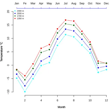
Figure 2.5: Monthly mean temperature derived from Storm meteo stations in four studied sites in 2013 (each points shows the monthly mean).
1400 1600 1800 2000 2200 0 2 4 6 8 Day of year Mean T emper ature °C R²=0.97 T=−0.0054Alt+14.34
Figure 2.6: Plot of comparison the annual mean temperature derived from Storm local Meteo stations.
within a day. The plots of daily mean temperature have been compared for each individual site and also along the gradient. The results of regression analysis for the mean temperature of the period in which the data were recorded by dendrometers (from January to November) showed a decrease in temperature with increasing
al-titude (T = −0.0054Alt + 17, R2 = 0.96, P = 0.002). The observed trend can be
stated as a decrease of 0.54◦ per 100 m increase in altitude (figure 2.7).
● ● ● ● ● ● ● ● ● ● Month T emper ature °C ● ● ● ● ● ● ● ● ● ● ● ● ● ● ● ● ● ● ● ● ● ● ● ● ● ● ● ● ● ● 2 4 6 8 10 Month T emper ature °C −10 −5 0 5 10 15 20
Jan Fe Mar Apr May Jun Jul Aug Sep Oct
2300 m 2000 m 1700 m 1350 m
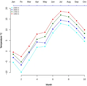
Figure 2.7: Monthly mean temperature recorded at tree stem in four studied sites in 2013 (each points shows the monthly mean).
Comparison of temperature data derived from different sources
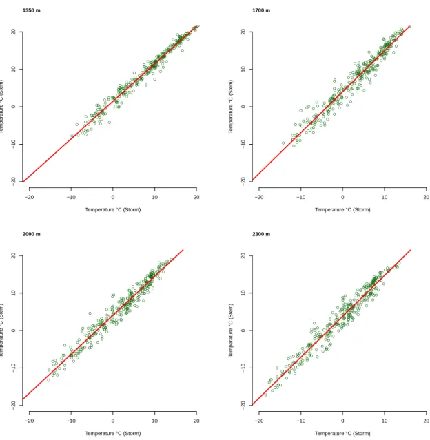
The comparison of temperature data from Storm local climate stations and the data recorded at tree stem showed a strong accordance and significant regression analysis
(P< 0.0001, (R2 > 0.90) (figure 2.8). Since the data derived from Storm data set
and the data at tree stem showed good accordance we used the Storm data base as the main resource of temperature.
Temperature derived from Meteo-France data base
Temperature data were also obtained from Meteo-France climate stations of “Vil-lard St. Pancrace”, “LE MONETIER LES BAINS”, and “MONTGENEVRE” close
● ● ● ● ● ● ● ● ● ● ● ● ● ● ●● ● ● ● ● ● ● ●● ● ● ● ● ● ● ● ● ● ● ● ● ● ● ● ● ● ● ● ●● ● ● ● ● ● ● ● ● ● ● ● ● ● ● ● ● ● ● ● ● ● ● ● ●●● ● ● ● ● ● ● ● ● ● ● ● ● ● ● ● ● ● ● ● ● ● ● ● ● ●● ● ● ● ●● ● ● ● ●●● ● ● ● ●● ● ● ● ● ●● ● ● ● ●●●● ● ● ● ● ●● ● ● ● ●● ● ● ● ● ● ● ● ● ● ● ● ● ● ● ● ● ● ● ● ●●● ● ● ● ● ● ● ● ● ●● ● ● ● ● ● ● ●●● ●● ● ● ● ● ● ● ● ● ● ● ● ● ● ● ● ● ● ● ● ● ● ● ● ● ● ●●● ● ● ● ● ●● ● ●● ● ● ● ● ●● ● ● ●●●●● ● ●●● ● ● ● ● ● ● ● ● ● ●● ● ● ● ●● ● ●● ● ● ● ● ● ● ● ● ● ●●● ●● ●● ● ● ● ●● ● ● ● ● ●● ● ● ● ● ● ● ●● ● ● ●● ● ● ● ● ● ● ● ● ● ● ● ● Temperature °C (Storm) T emper ature °C (Stem) −20 −10 0 10 20 −20 −10 0 10 20 1350 m ● ● ● ● ● ● ● ● ● ● ● ● ● ● ● ● ● ● ● ● ● ● ●● ● ● ● ● ● ● ● ● ● ● ● ● ● ● ● ● ●● ● ● ● ● ● ● ● ● ● ● ● ● ● ● ● ● ● ● ●● ● ● ● ● ● ●●● ● ● ●● ● ● ●● ● ● ● ● ● ● ● ● ● ● ● ● ● ●● ● ●● ● ● ● ● ● ● ● ● ● ●● ● ● ● ● ● ● ● ● ● ● ● ● ● ● ● ●●●●● ● ● ● ● ● ● ● ● ● ● ● ● ● ● ● ● ● ● ● ● ● ● ● ● ● ● ● ●● ● ● ● ● ● ● ● ● ● ● ● ●● ● ● ●● ● ● ●● ● ●● ● ● ●● ● ● ● ● ● ●● ●● ● ● ● ● ● ● ● ● ● ● ● ● ●● ● ● ● ● ●●● ●●● ● ● ● ● ●● ● ● ● ● ●● ● ● ● ● ● ● ● ● ● ●● ●● ●●● ●●● ● ● ● ● ● ● ● ● ● ● ● ● ● ● ● ● ● ●● ● ● ● ● ● ● ● ● ●● ●● ●●● ● ● ● ● ● ● ● ● ● ● ● ● ●● ● ● ● ● ● ● ● ● Temperature °C (Storm) T emper ature °C (Stem) −20 −10 0 10 20 −20 −10 0 10 20 1700 m ● ● ● ● ● ● ● ● ● ● ● ● ● ● ● ● ● ● ●●● ● ●●● ● ● ● ● ● ●● ● ● ● ● ● ● ● ● ● ● ● ● ● ● ● ● ● ● ● ● ● ● ● ●● ● ● ● ●●● ● ● ● ● ● ●● ● ● ● ● ● ● ● ● ● ● ● ● ● ● ● ● ● ● ● ● ● ● ● ● ● ●● ● ● ● ●●● ●● ● ● ● ● ● ● ● ● ● ● ● ● ● ● ● ● ● ● ● ● ● ● ● ● ● ● ● ● ● ● ● ● ● ●● ● ● ● ● ● ● ● ● ● ● ● ●● ● ● ● ●● ● ● ● ● ● ● ● ● ● ● ● ● ● ● ● ● ● ●●● ● ● ● ● ● ● ● ● ● ● ● ●● ● ● ● ● ● ● ● ●● ● ● ● ● ● ●● ● ● ● ● ●● ● ●●● ● ● ●● ●● ●● ● ● ●● ● ● ● ● ● ● ● ● ● ● ● ●● ● ● ● ●● ● ● ● ● ●● ● ● ● ● ● ● ● ● ● ● ● ● ●● ● ● ● ● ● ● ●● ● ● ● ●●● ● ● ● ● ● ● ● ● ●● ● ● ● ● ● ●● ● ● ● ● ● ● Temperature °C (Storm) T emper ature °C (Stem) −20 −10 0 10 20 −20 −10 0 10 20 2000 m ● ● ● ● ● ● ● ● ● ● ● ● ● ● ● ● ● ● ● ● ● ●●● ● ● ● ● ● ● ● ● ● ● ● ● ● ● ● ● ● ● ● ● ● ● ● ● ● ● ● ● ● ● ● ●● ● ●● ● ● ● ● ● ● ● ● ● ● ● ● ● ● ● ●● ● ● ● ● ● ● ● ● ● ● ● ● ● ● ● ● ●● ● ● ● ● ● ● ● ● ● ● ●●● ● ● ● ● ● ● ● ● ● ●● ● ● ● ● ● ● ● ●● ● ● ● ● ● ● ● ● ● ● ●● ● ● ● ● ● ● ● ● ● ● ● ● ● ● ● ● ●● ● ● ● ● ● ● ●● ● ● ● ● ● ● ● ● ● ●●● ● ● ● ● ● ● ● ●● ● ● ●● ● ● ● ● ●● ● ● ● ● ●●● ● ●●● ● ● ● ●● ● ● ● ● ● ● ● ● ● ●●● ● ● ●● ● ● ● ● ● ● ● ●●●● ● ● ● ● ● ● ● ● ●● ● ● ● ● ● ● ● ● ● ● ● ● ●● ● ●● ● ● ● ● ● ● ● ● ● ● ● ●● ● ● ● ● ● ●● ● ● ● ● ● ● ● ● ● ● ● ● ● ● ● ● ● Temperature °C (Storm) T emper ature °C (Stem) −20 −10 0 10 20 −20 −10 0 10 20 2300 m
Figure 2.8: Plot of comparison the temperature data derived from dendrometer and Storm local station at the sites of 1350 m, 1700 m, 2000 m and 2300 m.
to our study site in Briançon (table 2.3). The daily minimum, maximum tempera-ture were extracted from Meteo France stations. The daily mean temperatempera-ture was computed by taking the average of minimum and maximum for each day (figure 2.9).
Table 2.3: Geographical position of Meteo-France Stations close to Briançon
Site Latitude Longitude Altitude
Villard St.Pancrace 44◦52048"N 6◦38024"E 1310 m
LE MONETIER LES BAINS 44◦58012"N 6◦30048"E 1459 m
MONTGENEVRE 44◦55048"N 6◦43012"E 1848 m ● ● ● ● ● ● ● ● ● ● ● ● Month T emper ature °C ● ● ● ● ● ● ● ● ● ● ● ● ● ● ● ● ● ● ● ● ● ● ● ●
Jan Fe Mar Apr May Jun Jul Aug Sep Oct Nov Dec
MONETIER MONTGENEVRE Villard 2 4 6 8 10 12 Month T emper ature °C −15 −10 −5 0 5 10 15 20
Figure 2.9: Plot of comparison the monthly mean temperature recorded by Meteo France stations.
Comparison of temperature data derived from Storm and Meteo France dataset
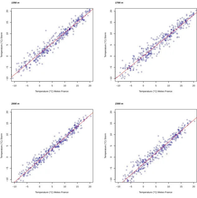
The comparison of Meteo-France stations also showed a good accordance with other resources of temperature so they were considered as good resources for obtaining
other climatic data such as precipitation (P< 0.001, R2 > 0.90) (figure 2.10).
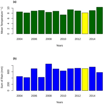
Temperature status along gradient
In order to see if the study year (2013) had a significant different climate, the long term comparison of temperature and precipitation data (2004 to 2015) have been done. The results of this comparison revealed that the study year 2013 was a normal year (figure 2.11).
● ● ● ● ● ● ● ● ● ● ● ●● ● ● ● ● ● ● ●● ●● ● ● ● ● ● ● ● ● ● ● ● ● ● ● ● ● ● ● ● ● ● ● ● ●● ● ● ● ● ● ● ● ● ● ● ● ● ● ● ● ● ● ● ● ● ●● ● ● ● ● ● ● ● ● ● ● ● ● ● ● ● ●● ● ● ● ● ● ● ● ● ● ● ● ● ● ● ● ● ● ● ● ●● ● ● ● ● ● ● ● ● ● ● ● ● ● ● ● ● ● ● ● ● ● ● ● ● ● ● ● ● ● ● ● ● ● ● ● ● ● ● ● ● ● ● ● ● ● ● ● ●● ● ● ● ● ● ● ● ● ● ● ● ● ● ● ● ●● ● ● ●● ● ● ● ●● ● ● ● ● ● ● ● ● ● ● ●● ● ● ● ● ● ● ● ● ● ● ● ●● ● ● ● ● ● ●● ● ● ● ● ● ● ●● ● ● ●● ●●● ● ● ●● ● ● ● ● ● ● ● ●● ● ● ● ● ● ● ● ● ● ● ● ● ● ● ● ●● ● ● ●● ● ● ● ● ● ● ● ● ● ●● ●● ● ● ● ● ● ● ● ● ● ● ● ● ● ● ● ● ● ● ● ● ●● ● ● ● ● ● ● ● ● ● ● ● ● ● ● ● ● ● ● ● ● ● ● ● ● ● ● ● ● ● ● ●● ●● ● ● ● ● ● ● ● ● ● ● ● ● ● ● ● ● ● ● ● ● ● ● ● ● ● ● ● ● ● ● ● ● −10 −5 0 5 10 15 20 −10 −5 0 5 10 15 20
Temperature (°C) Meteo France
T emper ature (°C) Stor m 1350 m ● ● ● ● ● ● ● ● ● ● ● ●● ●● ● ● ● ● ● ● ●● ● ● ● ● ● ● ● ● ● ● ● ● ● ● ● ● ●● ● ● ● ● ● ●● ● ● ● ● ● ● ● ● ● ● ● ● ● ● ● ● ● ● ● ● ● ● ● ● ● ● ● ● ● ● ● ● ● ● ● ● ● ● ● ● ● ● ● ● ● ●● ● ● ● ● ● ● ● ● ● ● ●● ● ● ● ● ● ● ● ● ● ● ● ● ● ●● ● ●● ● ● ● ● ● ● ● ● ● ● ● ● ● ● ● ● ● ● ● ● ● ● ● ● ● ● ● ● ● ●● ● ● ● ● ● ● ● ● ● ● ● ● ● ● ● ● ● ● ● ● ●● ● ● ● ● ● ● ● ● ● ● ● ● ● ●● ● ●● ● ● ● ● ● ● ● ● ● ●● ● ● ● ● ● ● ●● ● ● ● ● ● ● ● ● ● ● ● ● ●● ● ● ● ● ● ● ● ● ● ● ● ● ● ● ● ● ● ● ● ● ● ● ● ● ● ● ● ● ● ● ● ● ● ● ● ● ● ● ● ● ● ● ● ● ● ● ●● ● ● ● ● ● ● ● ● ● ● ● ● ● ● ● ● ● ● ● ● ● ● ● ● ● ● ● ●● ● ● ● ● ● ● ● ● ● ● ● ● ● ● ●● ● ● ●● ● ● ● ● ● ● ● ● ● ● ●● ● ● ● ● ● ● ● ● ● ● ● ● ● ● ●● ●● ● ● ● ● ● ● ● ● ● −10 −5 0 5 10 15 20 −10 −5 0 5 10 15 20
Temperature (°C) Meteo France
T emper ature (°C) Stor m 1700 m ● ● ● ● ● ● ● ● ● ● ● ● ● ● ● ● ● ● ● ● ● ● ● ● ● ● ● ● ● ● ● ● ● ● ● ● ● ● ● ● ● ● ● ● ●● ● ● ● ● ● ● ● ● ● ● ● ● ● ● ● ● ● ● ● ● ● ● ●● ● ● ● ● ● ● ● ●● ● ● ● ● ● ● ● ● ●● ● ● ●●●● ● ● ● ● ● ● ● ● ● ● ● ●● ● ● ● ●● ● ● ● ● ● ● ● ●●●●●● ● ● ● ● ● ● ● ● ●●● ●● ● ● ● ● ● ● ● ● ● ● ● ● ● ● ● ● ● ● ● ● ● ● ● ● ● ● ● ● ● ● ● ● ● ● ● ● ● ● ● ● ● ●● ● ● ● ● ● ● ● ● ● ● ●● ● ● ● ● ●● ● ● ● ● ● ●● ● ● ● ● ●●● ● ● ● ● ● ● ● ●● ● ● ● ● ●● ● ● ● ● ● ● ● ● ● ● ● ● ●● ● ● ● ● ● ● ● ● ● ● ● ● ● ● ● ● ● ● ● ●● ● ● ● ● ● ● ● ● ● ● ● ● ● ● ● ● ● ● ● ● ● ● ● ● ● ● ● ● ● ● ● ● ● ● ● ● ● ● ● ● ● ● ● ● ● ● ● ● ● ● ● ● ● ● ● ● ● ● ● ● ●● ● ● ● ● ● ● ● ●● ● ● ● ● ● ● ● ● ● ● ● ● ● ● ● ● ● ●● ●● ● ● ● ● ● ● ● ● ● −10 −5 0 5 10 15 20 −10 −5 0 5 10 15 20
Temperature (°C) Meteo France
T emper ature (°C) Stor m 2000 m ● ● ● ● ● ●● ● ● ● ● ● ● ● ● ● ● ● ● ● ● ● ● ● ● ● ● ● ● ● ● ● ● ● ● ● ● ● ● ● ● ● ● ● ● ● ● ● ● ● ● ● ● ● ● ● ● ● ● ● ● ● ● ● ● ● ● ● ●● ● ● ● ● ● ● ● ●● ● ● ●● ● ● ● ● ● ● ● ● ●●●● ● ● ● ● ● ● ● ● ● ● ● ● ● ● ● ● ● ● ● ● ● ● ● ● ● ●● ● ● ● ● ● ● ● ● ● ● ● ● ●●● ●● ● ● ● ● ● ● ● ● ● ● ● ● ● ● ● ● ● ● ● ● ● ● ● ● ●●● ● ● ● ● ● ● ● ● ● ● ● ● ● ● ●●●● ● ● ● ● ● ● ● ● ● ● ● ● ● ● ● ● ● ● ● ● ● ●● ● ● ● ● ●● ● ● ● ● ● ● ●● ● ● ● ● ● ● ●● ● ● ● ● ● ● ● ● ● ● ● ● ●● ● ● ● ● ● ● ● ● ● ● ● ● ● ● ● ● ● ● ● ●● ● ●● ● ● ● ● ● ●● ● ● ● ● ● ● ● ● ● ● ● ● ● ● ● ● ● ● ● ● ● ● ● ● ● ●● ● ● ● ● ● ● ●● ● ● ● ● ● ● ● ● ● ● ● ● ● ● ● ● ● ● ● ● ● ● ● ● ● ● ● ● ● ● ● ● ● ● ●● ● ● ● ● ● ● ● ● ● ● ● ● ● ● ● ● ● ● ● ● −10 −5 0 5 10 15 20 −10 −5 0 5 10 15 20
Temperature (°C) Meteo France
T
emper
ature (°C) Stor
m
2300 m
Figure 2.10: Plot of comparison the temperature data derived from MeteoFrance and Storm local station at the sites of 1350 m, 1700 m, 2000 m and 2300 m.
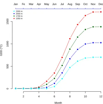
Computing growing degree days
Growing degree days (GDD) is the measurement of heat accumulation that is usually used to estimate the growth and development of plants during the growing season. The basic concept is that development will only occur if the temperature exceeds a minimum threshold known as T base. The GDD is usually computed using the
base temperature of 5 ◦ C (Bonhomme 2000). The growing degree days (GDD)
was computed for selected plot in 1350, 1700, 2000, 2300 m based on following