A Large Area Micromegas TPC for Tracking at the ILC

HAL Id: tel-00854414

https://tel.archives-ouvertes.fr/tel-00854414

HAL is a multi-disciplinary open access

archive for the deposit and dissemination of sci-entific research documents, whether they are pub-lished or not. The documents may come from teaching and research institutions in France or abroad, or from public or private research centers.

L’archive ouverte pluridisciplinaire HAL, est destinée au dépôt et à la diffusion de documents scientifiques de niveau recherche, publiés ou non, émanant des établissements d’enseignement et de recherche français ou étrangers, des laboratoires publics ou privés.

A Large Area Micromegas TPC for Tracking at the ILC

Wenxin Wang

To cite this version:

Wenxin Wang. A Large Area Micromegas TPC for Tracking at the ILC. Other [cond-mat.other]. Université Paris Sud - Paris XI, 2013. English. �NNT : 2013PA112099�. �tel-00854414�

1

UNIVERSITE PARIS-SUD

ÉCOLE DOCTORALE :

Faculté des sciences d’Orsay

DISCIPLINE : Physique des particules

THÈSE DE DOCTORAT soutenue le 24/06/2013

par

Wenxin WANG

Etude d’un grand détecteur TPC

Micromegas pour l’ILC

Directeur de thèse : Dr Paul COLAS Chercheur, CEA-Saclay

Composition du jury :

Président du jury : Prof. Patrick PUZO Professeur, Université Paris Sud, Orsay

Rapporteurs : Dr DidierCONTARDO Chercheur, IPN Lyon, Université Claude Bernard Dr Gilles DE LENTDECKER Chercheur, Université Libre de Bruxelles Examinateurs : Dr Jan TIMMERMANS Chercheur, NIKHEF

3

University Paris-Sud

Graduate School 534 MIPEGE

Faculty of Sciences of Orsay

THESIS

Wenxin WANG

to obtain the degree of :

Doctor of the University Paris-Sud

Specialty

: Particle Physics

A Large Area Micromegas TPC for

Tracking at the ILC

SUPERVISOR :

Dr COLAS Paul Researcher, CEA-Saclay

REVIEWERS :

Dr CONTARDO Didier Researcher, IPN Lyon, Université Claude Bernard

Dr DE LENTDECKER Gilles Researcher, Université Libre de Bruxelles

EXAMINERS :

Prof. PUZO Patrick Professer, Université Paris Sud, Orsay

Dr TIMMERMANS Jan Researcher, NIKHEF

5

To m y parents A m es parents 致我的父母

7

Acknowledgements

It’s hard to express how grateful I am just in a few words. These years in France will remain permanently in my memory. I have been so lucky to work in this wonderful group with so great people.

Firstly, I would like to thank my PhD supervisor, Dr Paul COLAS, who is always so kind and so patient to give me the guidance and advice, provide me so good chance to really see the world of experimental physics. I also would like to thank David ATTIE who provided me a lot of help during my research. He is so smart person. Each time, when I discussed with him, I made a big step in my work. Thanks to the electronics group, they did very beautiful job and provided very good electronics so that my experiment was going so smoothly. I also thank Marc RIALLOT and other people who work at SEDI. When I met problems and my colleagues of my group were not around, they always gave me unconditional help.

I also would like to thank Ursula BASSLER, leader of the Irfu particle physics division, for her welcome at SPP, and Georges VASSEUR, my godfather, for his support.

My thanks go also to Didier CONTARDO, Gilles DE LENTDECKER, Patrick PUZO, Jan TIMMERMANS, and Didier VILANOVA for accepting to judge this thesis.

Outside my institute, I thank all the people who are working in our collaboration: Madhu DIXIT, Keisuke FUJII, and the students who were working with them, as well as the DESY group.

Thanks very much to the people who gave me tremendous help for my French. I’m not good at learning foreign languages. They were so patient to speak with me. Also, I would like to thank my Chinese friends. They gave me a lot of help.

Without you all, it would have been hard for me to live in France, to complete my PhD work. I really appreciate all your help for the last years.

9

Résumé

Une grande ‘Chambre à Projection Temporelle’ (TPC) est un candidat pour la détection et la mesure des traces chargées auprès de l’ILC, collisionneur linéaire d’électrons et de positons de 31 km permettant d’atteindre des énergies dans le centre de masse de 250 GeV à 1 TeV. Le travail de R&D décrit dans cette thèse porte sur un type nouveau de TPC, dont la lecture est assurée par des Micromégas à anode résistive. Ce dispositif permet de répartir le signal électrique sur plusieurs carreaux, même lorsque la charge est déposée sur un seul carreau. Il permet aussi de protéger l’électronique, ce qui est utilisé dans notre prototype pour miniaturiser les cartes de lecture.

Dans ce travail, des modules Micromégas ont été testés et caractérisés, dans un premier temps, en faisceau, un par un au centre de la chambre, puis 7 modules montés en même temps de façon à couvrir la surface. Egalement, des tests sur un banc équipé d’une source de

55

Fe ont permis de caractériser les 7 modules utilisés. Une résolution en position de 60 microns par ligne de carreaux est obtenue à petite distance de dérive. L’uniformité est aussi évaluée, et des distorsions pouvant atteindre environ 500 microns sont observées.

L’ensemble des résultats démontre l’adéquation de ce type de lecture à la TPC pour l’ILC. La fraction de retour des ions est également mesurée à l’aide d’un détecteur de même géométrie et avec le même gaz que ceux utilisés dans ces tests, et la loi en rapport inverse des champs est validée à nouveau dans ces conditions.

La même technique est appliquée à la réalisation d’un imageur neutron, consistant en une TPC Micromégas ‘plate’ précédée d’un film convertisseur de 1mm d’épaisseur. Les protons éjectés par les neutrons sont ‘suivis à la trace’ dans le volume gazeux, ce qui permet de reconstruire avec une précision meilleure que le millimètre le point d’origine du neutron.

Mots-clés : trajectographie, lecture à anode résistive, Micromégas, Chambre à Projection Temporelle (TPC)

11

Résumé de thèse

L’étude des composants fondamentaux de la matière nécessite des accélérateurs toujours de plus en plus puissants. De nouvelles particules sont produites dans les collisions à haute énergie de protons ou d’électrons. Les produits de ces collisions sont détectés dans de grands appareillages entourant le point d’interaction. La particule de Higgs de 125 GeV découverte au LHC sera étudiée en détails au futur collisionneur e+e-. Le projet phare dans ce domaine est appelé ILC, pour ‘Collisionneur Linéaire International’. L’équipe que j’ai rejointe à Saclay travaille depuis une douzaine d’années sur un projet de grande ‘Chambre à Projection Temporelle’ (TPC) pour détecter les traces chargées à l’aide de l’ionisation qu’elles laissent dans un volume de gaz. Cette TPC d’un type nouveau est adaptée à l’utilisation dans les conditions de l’ILC. Les électrons d’ionisation dérivent aux deux extrémités de la chambre sous l’action d’un champ électrique. Ils sont multipliés par un dispositif Micromegas, équipé d’une anode à étalement de charge faite d’un revêtement résistif-capacitif.

Le collisionneur ILC est une machine constituée de deux accélérateurs linéaires face-à-face, d’une longueur totale de 31 km. Les éléments accélérateurs sont des cavités supraconductrices. Un grand anneau d’amortissement situé au milieu est partagé entre les électrons et les positons.

Depuis la découverte d’une particule de 125 GeV au LHC, annoncée le 4 juillet dernier, et qui vérifie, à la précision actuelle des mesures, toutes les propriétés attendues d’un boson de Higgs, la nécessité de l’étudier d’une façon plus propre et plus indépendante du modèle se fait sentir. Le processus de Bjorken (aussi appelé Higgs-strahlung, voir Fig. 1-3 produira des Higgs avec une section efficace de 250 fb (Fig. 1.1). La signature du recul du Z, se désintégrant en paire de muons permettra de sélectionner les candidats Higgs quelque soit son mode de désintégration, et aussi de mesurer précisément sa masse et ses rapports d’embranchement, et ainsi de remonter à ses différents couplages. La TPC joue un rôle important dans cette analyse et permet de mesurer précisément les particules chargées et de les associer précisément avec des objets calorimétriques, ce qui est essentiel à la mise en œuvre de l’algorithme du « flux de particules », qui consiste à faire un bilan précis du contenu en énergie-impulsion des objets reconstruits dans le détecteur, en évitant tout double-comptage.

12

Figure R-1. A gauche, diagramme de Feynman du processus de Higgs-strahlung; à droite, événement simulé de top-antitop multijet.

Les principales propriétés des TPC sont rappelées dans le chapitre 2. Les processus de dérive et de diffusion des électrons sont étudiés, en présence d’un champ magnétique. L’amplification gazeuse et, en particulier, le cas de Micromégas sont traités. Le processus de production de la version ‘bulk’ (tout-en-un) de ce détecteur par méthode photo-lithographique est décrit. Une section est réservée à la présentation de la technique d’anode résistive, propre à notre application : la taille typique d’une avalanche n’excédant pas 15 à 20 microns, le signal n’est généralement pas partagé sur des damiers de 2 à 3 mm de large. L’ajout d’une couverture résistive au-dessus des pads, séparée de ceux-ci par une couche diélectrique, résulte en un réseau résistif-capacitif continu. Toute charge ponctuelle déposée sur la surface s’étale. La densité de charge suit l’équation de diffusion à deux dimensions (2-0-20), dont la solution est une gaussienne à deux dimension dont le rayon croît comme la racine carrée du temps. La valeur de la constante de temps RC par unité de surface doit être ajustée pour obtenir l’étalement optimum : deux ou trois pads sur la durée typique des signaux détectés.

13

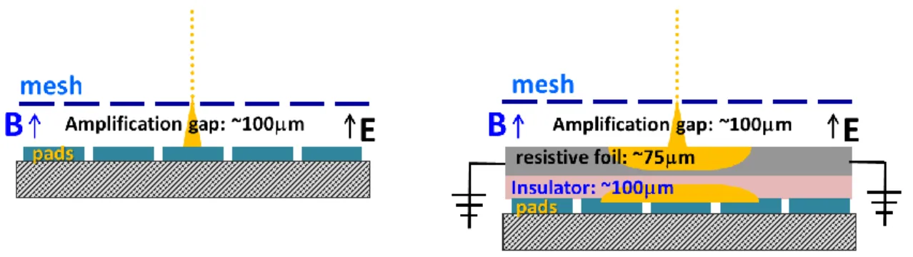
Figure R-2. A gauche, Micromegas à anode conventionnelle, le signal est sur un seul carreau; à droite, le revêtement résistif-capacitif étale la charge sur plusieurs carreaux.

Le chapitre 3 décrit l’appareillage utilisé lors des tests en faisceaux. Après une présentation de la collaboration LCTPC et du Grand Prototype construit par le consortium EUDET, je décris les modules mis au point dans notre groupe et l’électronique de lecture AFTER conçue à Saclay. Dans ce même chapitre la détermination des piédestaux et leur soustraction en ligne sont présentés. Les piédestaux et leur écart quadratique moyen sont calculés sur la base de quelques centaines d’événements déclenchés aléatoirement. Le piédestal est soustrait et seuls les signaux supérieurs à quatre écarts standard sont conservés (les autres sont mis à zéro). Ceci permet de diminuer notablement l’espace disque occupé par les données.

14

Pour rendre possible l’intégration du détecteur final, une miniaturisation de l’électronique s’est avérée nécessaire. Les puces AFTER ont été directement câblées sur des cartes reliées au détecteur par des connecteurs 300 points, et tous les composants visant à la protection de l’électronique ont été retirés, cette fonction étant assurée par la couche résistive. Pour terminer ce chapitre, le passage du prototype à la TPC finale est traité.

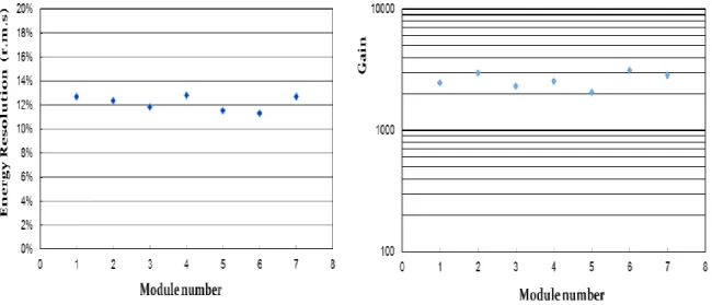
Dans le chapitre 4, le banc de test installé au CERN est décrit. Ce banc de test a été utilisé pour caractériser et tester tous les modules après fabrication. Des statistiques sur le gain et la résolution sont obtenues à partir de données obtenues avec source de 55Fe pour 7 modules. Pour cette mesure, le bruit électronique a été considérablement réduit par l’introduction d’un filtre en T (filtre passe-haut) sur l’alimentation de la grille.

La résolution (12 à 13% r.m.s.) et le gain (2640 avec un étalement de 15%) sont assez homogènes pour les 7 modules. Cette mesure de gain est en accord avec celle obtenue à l’aide des électrons du faisceau.

Figure R-4. Résolution en énergie et gain mesurés sur le banc de test pour chacun des 7 modules.

Le problème du retour des ions est récurrent dans les TPC. Dans les TPC conventionnelles, à fils, 20 à 30% des ions créés près des fils remontent en direction de l’espace de dérive. Les ions dérivant beaucoup plus lentement que les électrons et en sens inverse, il en résulte l’accumulation d’une charge d’espace dans la zone de dérive, susceptible de dévier les électrons d’ionisation au cours de leur dérive et donc d’introduire des distorsions. Des

15

mesures ont été effectuées il y a une dizaine d’années dans le groupe Micromégas, accompagnée d’une explication théorique du phénomène, et ces mesures concluaient à une suppression du retour des ions d’un facteur proportionnel au rapport des champs (amplification / dérive). Ces études avaient été faites avec des Micromegas standard (50 microns d’épaisseur de gaz) alimentées en mélange Ar+10% CH4. J’ai réitéré ces mesures

avec des bulk standards de 128 microns et du gaz T2K, à l’aide d’un canon à rayons x. J’ai bien retrouvé la dépendance attendue en rapport inverse des champs. J’ai également mesuré l’efficacité de collection (signal en fonction du rapport des champs) et étudié la dépendance de la résolution sur l’énergie en fonction de ce rapport des champs à gain constant.

Figure R-5. La fraction de retour des ions en fonction du rapport du champ d’amplification au champ de dérive.

Dans le chapitre 6, le logiciel d’analyse est décrit en détails. La fonction de réponse des pads est définie: fraction du signal présente sur un carreau de lecture en fonction de la distance du centre de ce carreau de lecture à la trace. Cette distribution est paramétrée, puis ajustée sur des données dans un processus itératif (la trace s’améliore au cours des itérations). Principalement deux paramétrages ont été utilisés : une à quatre paramètres (rapport de deux polynômes d’ordre 4, et une à deux paramètres, combinaison d’une gaussienne et d’une lorentzienne. La deuxième permet une convergence beaucoup plus rapide de l’ajustement des paramètres. Pour déterminer la résolution et se débarrasser d’éventuels effets d’inhomogénéité de la couche résistive-capacitive, le biais (valeur moyenne des résidus) est corrigé au cours de ces itérations, et la trace ré-ajustée.

16

La géométrie du détecteur, très importante pour l’étude des distorsions, est décrite ainsi que son implémentation. Les carreaux d’une même rangée sont associés entre eux s’ils sont contigüs, pour former un hit. La méthode de reconstruction, basée sur le filtre de Kalman, consiste à tenter d’associer des hits voisins en ensembles continus pour former des traces. Un critère de variation de ² est utilisé pour accepter ou rejeter un nouveau hit dans une trace. L’association de nouveaux hits se fait d’abord de l’intérieur vers l’extérieur, puis un second passage, de l’extérieur vers l’intérieur, permet d’associer les hits non utilisés. La description détaillée de l’algorithme est effectuée en appendice. Dans l’état actuel de l’algorithme, toutes les rangées sont affectées de la même incertitude dans le calcul du ². Cependant, si un hit est très loin de la trace (c’est le cas pour les électrons delta, émis perpendiculairement à la trace, ou, plus rarement, pour les carreaux bruyants) ce point est affecté d’une grande erreur pour qu’il ne tire pas la trace vers lui. Ceci est illustré au chapitre 7 consacré à la présentation des résultats des tests en faisceaux.

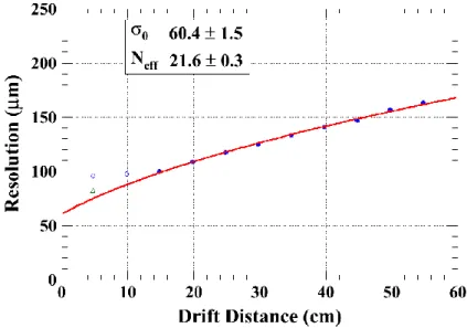
Figure R-6. Résolution moyenne des 22 lignes centrales en fonction de la distance de dérive. La courbe rouge est un ajustement de la fonction 7-0-2. Les points ouverts ne sont pas pris

17

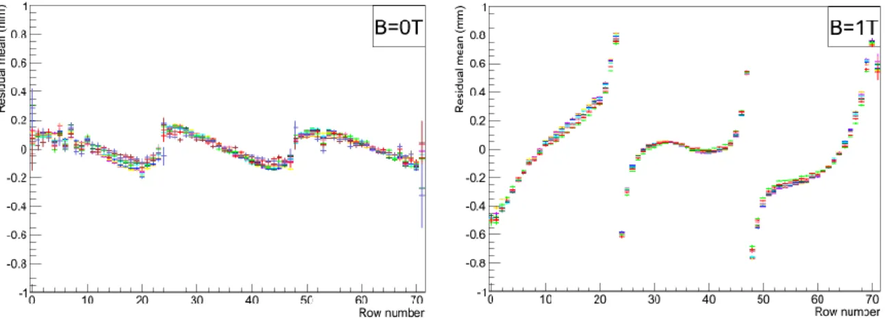
Figure R-7. Valeur moyenne des résidus en fonction du numéro de ligne, dans les cas sans et avec champ magnétique.

La résolution est ainsi déterminée en fonction de la distance de dérive. La résolution à distance zéro est de 60 microns, ce qui est un record pour des carreaux de 3mm de large. La comparaison ligne par ligne de cette résolution montre qu’elle est très uniforme, à part les lignes extrêmes (bords haut et bas des modules) pour lesquelles elle est de 50% au-dessus de la moyenne.

L’étude des résidus moyens pour des traces qui traversent trois modules mettent en évidence des distorsions pouvant atteindre 700 microns.

Le chapitre 8 est consacré au test d’un nouveau type d’imageur neutron, consistant en une TPC Micromégas ‘plate’. Un film de polyéthylène de 1mm d’épaisseur est utilisé comme convertisseur, et les protons éjectés par les neutrons sont ‘suivis à la trace’ dans le volume gazeux, ce qui permet de reconstruire avec une précision meilleure que le millimètre le point d’origine du neutron. Nous avons testé ce détecteur en Chine, avec l’équipe du Professeur Xiaodong Zhang, de l’Université de Lanzhou.

Quelques images obtenues avec un filtre de polyéthylène gravé sont montrées, et l’amélioration de la résolution avec l’extrapolation de la trace est clairement visible.

18

(a) (b)

Figure R-8. Image obtenue par neutrons à travers un filtre de polyéthylène, sans et avec la coupure en temps maximum.

19

Summary

The study of the fundamental building blocks of matter necessitates always more powerful accelerators. New particles are produced in high energy collisions of protons or electrons. The by-products of these collisions are detected in large apparatus surrounding the interaction point. The 125 GeV Higgs particle discovered at LHC will be studied in detail in the next e+e -collider. The leading project for this is called ILC. The team that I joined is working on the R&D for a Time Projection Chamber (TPC) to detect the charged tracks by the ionization they leave in a gas volume, optimised for use at ILC. This primary ionization is amplified by the so-called Micromegas device, with a charge-sharing anode made of a resistive-capacitive coating.

After a presentation of the physics motivation for the ILC and ILD detector, I will review the principle of operation of a TPC (Chapter 2) and underline the advantages of the Micromegas readout with charge sharing. The main part of this PhD work concerns the detailed study of up to 12 prototypes of various kinds. The modules and their readout electronics are described in Chapter 3. A test-bench setup has been assembled at CERN (Chapter 4) to study the response to a 55Fe source, allowing an energy calibration and a uniformity study. In Chapter 5, the ion backflow is studied using a bulk Micromegas and the gas gain is measured using a calibrated electronics chain. With the same setup, the electron transparency is measured as a function of the field ratio (drift/amplification).

Also, several beam tests have been carried out at DESY with a 5 GeV electron beam in a 1 T superconducting magnet. These beam tests allowed the detailed study of the spatial resolution. In the final test, the endplate was equipped with seven modules, bringing sensitivity to misalignment and distortions. Such a study required software developments (Chapter 6) to make optimal use of the charge sharing and to reconstruct multiple tracks through several modules with a Kalman Filter algorithm. The results of these studies are given in Chapter 7.

The TPC technique has been applied to neutron imaging in collaboration with the University of Lanzhou. A test using a neutron source has been carried out in China. The results are reported in Chapter 8.

21

Contents

1.1. A Linear Collider ... 33 1.2. Physics at the ILC ... 34 1.3. The ILC Machine Design ... 37 The ILD Detector Concept ... 39 2.

2.1. Particle Flow Concept ... 40 2.2. The ILD Detector Layout ... 41 2.3. Requirements to the Tracking System ... 42 Chapter 2 Time projection chamber principles ... 45 Principles of the TPC ... 47 1.

1.1. Drift ... 47 1.2. Diffusion ... 48 1.3. Gas amplification ... 50 Micromegas general introduction ... 50 2.

2.1. Micromegas TPC ... 51 2.2. Resistive anode ... 51 Chapter 3 Test-beam setup and Micromegas modules ... 55 LCTPC collaboration and EUDET ... 57 1.

Micromegas modules ... 62 2.

The AFTER chip ... 65 3.

The integrated electronics for ILC-TPC ... 73 4.

22

Calculation of the material budget of a module ... 75 5.

5.1. Definition of the radiation length ... 75 5.2. The materials of one module ... 76 5.3. Average thickness in radiation length of a module ... 76 Towards the ILD TPC ... 77 6.

Chapter 4 Test bench of Micromegas modules ... 79 Introduction of the test-bench ... 81 1.

Structure of the test bench ... 82 2. 55 Fe energy spectrum ... 85 3. Stability ... 86 4. Module comparison ... 87 5.

Chapter 5 Ion backflow measurement ... 89 Experimental setup ... 91 1.

Characteristics of the bulk Micromegas detector ... 92 2.

2.1. Gain ... 92 2.2. Energy resolution ... 92 2.3. Electron transparency ... 94 Ion backflow measurements ... 94 3.

Chapter 6 Analysis software ... 97 Introduction ... 99 1.

PRF (Pad Response Function)... 99 2. FTPC programme ... 101 3. 3.1. FTPC analysis chain ... 102 ILCSOFT ... 107 4.

Micromegas modules analysis chain in MarlinTPC ... 112 5.

Chapter 7 Analysis results ... 115 Gain study ... 117 1.

Drift velocity study ... 120 2.

Analysis with one module ... 121 3.

3.1. Uniformity of different modules ... 121 3.2. Spatial resolution ... 122 3.3. Optimization of the ADC accuracy ... 124 Analysis with multiple modules ... 125 4.

23

4.1. Missing pads ... 125 4.2. Distortions ... 127 4.3. Spatial resolution study ... 128 Conclusion ... 135 Chapter 8 Other Micromegas TPC application: imaging by neutrons ... 139 Detector description ... 141 1.

The characteristics measurements ... 142 2.

The neutron tests ... 143 3.

3.1. 241Am-9Be neutron source ... 143 3.2. Neutron imaging ... 144 Conclusion ... 147 4.

APPENDIX Kalman Filter in ILCSOFT ... 149 The principle of Kalman Filter ... 151 1.

Kalman Filter in ILCSOFT ... 153 2.

24

List of tables

Number Page

Table 1-1. Performance goals and design parameters for an LCTPC with standard electronics at the ILC detector. ... 43 Table 3-1. Some main test periods with the test modules. ... 59 Table 3-2. Characteristics of the AFTER chip. ... 67 Table 3-3. Radiation length of the materials of a module. ... 76 Table 6-1. Nominal module positions. ... 109 Table 6-2. MarlinTPC processors used for the Micromegas analysis. ... 111

25

List of figures

Number Page

Figure R-1. A gauche, diagramme de Feynman du processus de Higgs-strahlung; à droite, événement simulé de top-antitop multijet. ... 12 Figure R-2. A gauche, Micromegas à anode conventionnelle, le signal est sur un seul carreau;

à droite, le revêtement résistif-capacitif étale la charge sur plusieurs carreaux. ... 13 Figure R-3. Photographie du prototype 7 modules dans son aimant. ... 13 Figure R-4. Résolution en énergie et gain mesurés sur le banc de test pour chacun des 7

modules. ... 14 Figure R-5. La fraction de retour des ions en fonction du rapport du champ d’amplification au

champ de dérive. ... 15 Figure R-6. Résolution moyenne des 22 lignes centrales en fonction de la distance de dérive.

La courbe rouge est un ajustement de la fonction 7-0-2. Les points ouverts ne sont pas pris dans l’ajustement. ... 16 Figure R-7. Valeur moyenne des résidus en fonction du numéro de ligne, dans les cas sans et

avec champ magnétique. ... 17 Figure R-8. Image obtenue par neutrons à travers un filtre de polyéthylène, sans et avec la

coupure en temps maximum. ... 18 Figure 1-1. Production cross section of a 125 GeV SM Higgs boson as a function of with

80% polarization for the electrons and 20% polarization for the positrons. ... 35 Figure 1-2. Some production cross sections as a function of at e+

e- collider. ... 35 Figure 1-3. Diagrams for the Higgs production processes. (a) Higgs-strahlung process, (b)

WW fusion process, (c) ZZ fusion process, (d) radiation off tops process. ... 36 Figure 1-4. Simulated event - in the ILD detector. ... 36 Figure 1-5. Coupling of the Higgs boson to different SM particles. ... 37 Figure 1-6. International linear collider design. ... 37 Figure 1-7. Bunch structure of the ILC: 2625 bunches with 2 1010

particles in each bunch are arranged in a bunch train of about 1 ms length. The train repetition rate is 5 Hz . .... 38 Figure 1-8. International Large Detector concept. ... 39 Figure 1-9. One quadrant of the ILD detector concept with its subdetector systems . ... 41

26

Figure 2-1. (a) The structure of Micromegas detector. (b) Bulk Micromegas fabrication process. ... 51 Figure 2-2. Left: The conventional anode using directly signal readout technique. Right:

Charge dispersion technique with a resistive anode. ... 52 Figure 2-3. The evolution of the 2-dimensional charge density function at five different times. ... 53 Figure 3-1. Large Prototype (LP) with the movable stage in the beam area. ... 57 Figure 3-2. The field cage of LP-TPC. ... 59 Figure 3-3. The setup of the cosmic trigger. ... 60 Figure 3-4. The design of endplate of LP-TPC . ... 61 Figure 3-5. The Large Prototype with only one module installed in the center. ... 62 Figure 3-6. Seven identical modules mounted at the endplate of the Large Prototype. ... 63 Figure 3-7. The sketch of the readout pad of a Micromegas module with a typical track from

the beam. ... 63 Figure 3-8. Five Micromegas modules with different anode materials. ... 64 Figure 3-9. Left: Photograph of one module; Right: Structure of a module. ... 65 Figure 3-10. Front-end electronics of one Micromegas module . ... 66 Figure 3-11. Architecture of the AFTER chip . ... 67 Figure 3-12. 60 fC test pulses recorded by the AFTER chip (120 fC range) for 100 ns, 200 ns,

400ns, and 1 µs peaking times. ... 68 Figure 3-13. The uniformity of the ENC for the 1728 channels and a typical map of the r.m.s.

noise of the 1728 channels (24×72) of one detector module measured in the 120 fC range and with a 200 ns shaping time. ... 69 Figure 3-14. An example of the global value for the pedestal mean value and the r.m.s. value

histogram of 1728 channels. ... 70 Figure 3-15. Pedestal of the electronics. Each graph represents a 72-channel AFTER ASIC. 71 Figure 3-16. R.m.s. per channel measured with a Micromegas module. ... 72 Figure 3-17. The T2K electronics. (a) the packaging of electronics for one module test; (b)

one FEC (14 cm 25 cm ). ... 73 Figure 3-18. Artist view and photograph of the new FEC . ... 73 Figure 3-19. New integrated electronics split drawing of one module. ... 74 Figure 3-20. Micromegas module mounted with the new integrated electronics. ... 75

27

Figure 3-21. (a) An example of a model using Micromegas as the amplification system for the ILD-TPC; (b) An example of a model using GEM as the amplification system for the ILD-TPC . ... 77 Figure 4-1. The setup of the test bench. ... 81 Figure 4-2. The set of two mechanical arms which holds the 55Fe source. ... 82 Figure 4-3. The structure of the test bench. ... 82 Figure 4-4. The display of events using X-rays of 55Fe source and the corresponding

histogram of each pad’s ADC. (a) Before the filter was added between high voltage and mesh electrode; (b) After the filter was added between high voltage and mesh electrode. ... 83 Figure 4-5. (a) Collimated source (55Fe); (b) Source (55Fe) without collimator. ... 84 Figure 4-6. The map of disconnected pads in one of the modules. The disconnected pads are

in dark blue. ... 84 Figure 4-7. Mechanical problem: some studs de-soldered. ... 84 Figure 4-8. An example of X-rays event tested with collimator. ... 85 Figure 4-9. 55Fe energy spectrum. ... 85 Figure 4-10. Left: the distribution of gain over 16 hours. Right: the gain of the detector as a

function of time. ... 86 Figure 4-11. Left: the distribution of energy resolution over 16 hours. Right: the energy

resolution as a function of time. ... 87 Figure 4-12. Energy resolution and gain for different modules. ... 87 Figure 5-1. Experimental device (left hand) and schematic diagram of the set up (right hand)

for the ion backflow measurement. ... 91 Figure 5-2. Gain as a function of Vmesh for Edrift = 0.2 kV/cm at atmospheric pressure. ... 92

Figure 5-3. Measured 55Fe spectrum in a T2K gaseous mixture at Vmesh = 350 V and Vdrift =

400 V. ... 93 Figure 5-4. Energy resolution as a function of the ratio of Ed/Ea (Ed: drift electric field; Ea:

amplification electric field). ... 93 Figure 5-5. Electron transparency as a function of the ratio of Ed/Ea in the T2K gas mixture

(normalized to unity). ... 94 Figure 5-6. Ion backflow as a function of the field ratio of Ea/Ed. ... 95

Figure 6-1. An example of PRF for different drift distances . ... 100 Figure 6-2. The example of one track in the coordinate system. ... 101

28

Figure 6-3. The pad pulses. ... 103 Figure 6-4. PRF fitting. (a) top one: the scatter plot of the pad’s charge and the relative

position of the pad to the track; (b) bottom one: the fitting of the scatter points using PRF function. ... 104 Figure 6-5. Profile histogram of the residual with the track in one row before bias correction. ... 105 Figure 6-6. Profile histogram of the residual with the track in one row after bias correction. ... 106 Figure 6-7. Track parameters in MarlinTPC for a straight track. ... 108 Figure 6-8. Schematic overview of the modular structure of Marlin. ... 110 Figure 6-9. More than one track passes through module. The left one shows the tracks pass

through module 3 (the middle one at the endplate); the right one shows the signal recorded on the pad where two tracks cross. ... 113 Figure 7-1. The histogram of pads’ ADC in each row. ... 118 Figure 7-2. The distribution of effective number of electrons for 5 GeV electrons for a gas

thickness of 6.85 cm simulated by Heed . ... 118 Figure 7-3. Gain as a function of the mesh voltage. ... 118 Figure 7-4. Gain as a function of the mesh voltage with different drift electric fields. ... 119 Figure 7-5. Drift velocity measurements (B=0 T)... 120 Figure 7-6. Drift velocity measurements (B=1 T)... 121 Figure 7-7. Residual mean in µm for each row (from 0 to 23) at three different drift distances

with B = 1 T. Blue points are for the module with resistive ink anode and red points are for the module with carbon-loaded polyimide anode. ... 122 Figure 7-8. Measured resolution as a function of the drift distance Z at B=0 T (data taken with

200 ns peaking time): (a) module 4 (resistive kapton anode with a resistivity of about 3 M/), (b) module 5 (resistive kapton anode with a resistivity of about 3 M/). ... 123 Figure 7-9. Measured resolution as a function of the drift distance Z at B=1 T (data taken with

500 ns peaking time): (a) module 2 (resistive ink anode with a resistivity of about 3 M/), (b) module 3 (resistive kapton anode with a resistivity of about 5 M/). ... 124 Figure 7-10. Resolution as a function of ADC bits at different drift distances. ... 124 Figure 7-11. (a) Beam direction (b) Beam event. ... 125 Figure 7-12. The state of missing pads during first two days test. The missing pads are filled

29

Figure 7-13. The state of missing pads in the last-but-one data taking day. The missing pads are filled with white colour. ... 126 Figure 7-14. Left: the residual versus the row numbers in B=0 T. Right: the residual versus

the row numbers in B=1 T. Both are before bias correction. ... 127 Figure 7-15. Left: the residual mean versus the row numbers in B=0 T. Right: the residual

mean versus the row numbers in B=1 T. Different colours respond to different drift distances from 15 cm to 50 cm. ... 127 Figure 7-16. Examples of track fitting in one event. Left: multi-tracks in one event; Right:

signal track in one event. ... 128 Figure 7-17. Single track event. Left: display with 7 modules; Right: display with the centre

module (Zoom). ... 128 Figure 7-18. Fitting track using all hits in one track. (Red line: hit position; Blue line: fit track)

... 129 Figure 7-19. Fitting track with the error affected to the hit 35 set to a very large value so that it

does not weight in the chi-squared. (Red line: hit position; Blue line: fit track) ... 130 Figure 7-20. Fitting track after removing the hit in row 35 which has large residual. (Red line:

hit position; Blue line: fit track) ... 130 Figure 7-21. Distribution of the residuals at 15 cm drift distance. Top: including the test hit in

the track fit; Bottom: excluding the test hit in the track fit. Here only shows 3 rows of 72 rows. ... 131 Figure 7-22. Resolution of each row of the central module. ... 131 Figure 7-23. Spatial resolution of the central module at B=1 T. Data with seven modules

taken in 2013. ... 132 Figure 7-24. Extrapolation of the spatial resolutions of Micromegas and GEM to the ILD-TPC.

... 133 Figure 7-25. Resolution as a function of the crossing angle at different drift distances in B=1 T. ... 133 Figure 8-1. Sketch of the FNI detector. ... 141 Figure 8-2. The PCB of the neutron detector (sensitive area: 57.4 mm × 88.6 mm). ... 141 Figure 8-3. Energy resolution of the 55Fe spectrum. ... 142 Figure 8-4. Gas gain as a function of the mesh voltage in 95% Ar+5% isobutane. ... 143 Figure 8-5. 241Am-9Be source spectrum according to ISO 8529 standard. ... 144

30

Figure 8-6. The conversion efficiency as a function of the thickness of the polyethylene ([C2H4]n) layer simulated by Geant4. ... 144

Figure 8-7. Left: the setup of the neutron imaging test. Right: the corresponding imaging. . 145 Figure 8-8. Polyethylene masks used for the neutron imaging. ... 145 Figure 8-9. A typical neutron event with the maximum time and the minimum time in this

cluster. ... 146 Figure 8-10. Maximum time-difference in one cluster in 40 ns time bin. ... 146 Figure 8-11. Neutron imaging. (a) Integrating the ADC of all events in one pad. (b)

Reconstructed using the time information. ... 147 Figure 0-1. Geometric interpretation of the helix parameters for (a) negatively and (b)

31

Chapter 1

Introduction

33

The International Linear Collider Project

1.

The International Linear Collider (ILC) is a world-wide project for a future linear particle accelerator. The positron-electron (e+e-) beams will collide at the centre-of-mass (cms) energy of 200-500 GeV (with a possible later upgrade to 1 TeV). At present, the Large Hadron Collider (LHC) [1] is the world’s largest and highest-energy particle accelerator with high energy colliding proton beams. It is designed to reach centre-of-mass energies of 14 TeV with a high peak luminosity of 1034 cm-2s-1. The energy of the proton constituents is not fixed and partons collide with all possible energies. Thus a hadron collider covers a wide energy range at the constituent level while running at a fixed beam energy which makes them well suited as discovery machines. Its goals are to further test the Standard Model, determine what breaks the electroweak symmetry, search for new forces of nature, and produce dark matter candidates. But measurements at LHC cannot reach the highest precision. Firstly, the centre-of-mass energy is not adjustable and the initial energy of an interaction is unknown, as well as the precise kinematics. Secondly, the proton-proton interaction cross-section is dominated by inelastic background QCD processes. This means that each interesting signal event is accompanied by large backgrounds produced by the interaction of other parton collisions and it even overlaps with many other proton-proton collisions. The ILC, with its much lower experimental background, polarised beams, and tunable collision energies, will provide precision measurements regarding the LHC discoveries.

1.1.A Linear Collider

In a lepton collider, the initial state energy and the polarization are well known and could be changed. The interaction of electrons and positrons is purely electroweak and the Standard Model background is low. The requirements for radiation hardness are smaller compared to the LHC. This allows for high-precision detectors with low material budget.

To increase the energy to the required level, a linear collider instead of a circular collider will be needed. In a ring accelerator, the energy loss in one turn due to synchrotron radiation emitted by accelerated particles is

and for the electrons - .

Here, R is the curvature radius of the accelerator, m is the particle mass and E is the beam energy. The energy loss increases with the fourth power of the beam energy and decreases

34

only linearly with the radius. This makes a circular lepton collider unacceptably large if it is supposed to run beyond cms energy of √ GeV. Therefore the ILC will be a linear machine to avoid the synchrotron radiation losses.

1.2.Physics at the ILC

On July 4, 2012, both the CMS [2] and ATLAS [3] teams working at LHC announced the discovery of a new particle in the mass region around 125-126 GeV, with a statistical significance at the level of 5 sigma [4]. A 5-sigma result represents a one-in-3.5 million chance of the result being noise. This is an undeniable proof that a boson, with very Higgs-like properties, has been discovered by the two collaborations. However, a full characterisation of the Higgs includes a measurement of its total decay width, spin, production cross-section and coupling to the known Standard Model (SM) particles. These measurements are very difficult or impossible to perform at the LHC. The task of the ILC will be to measure precisely their properties. In contrast to hadron interactions, the collisions are characterised by much lower background and the ILC provides an accurate knowledge of the initial conditions like centre-of-mass energy, initial state helicity and charge. The ILC will be the first collider to reach the ̅ production threshold at around 350 GeV. This allows the mass and the electroweak properties of the top quark to be accurately measured.

At the ILC, one will measure the mass, spin, and coupling strengths through all decay channels. The main production mechanisms for SM-like Higgs particles at an collider are as follows. Figure 1-1 shows the production cross-section of a 125 GeV SM Higgs boson as a function of √ with 80% polarization for the electrons and 20% polarization for the

positrons and figure 1-2 shows some production cross sections as a function of √ .

a. Higgs-strahlung process:

b. WW fusion process: ̅ ̅ c. ZZ fusion process: d. Radiation off tops: ̅

Unseen intermediate states are indicated between parentheses. The corresponding diagrams of these Higgs production processes are shown in figure 1-3.

35

Figure 1-1. Production cross section of a 125 GeV SM Higgs boson as a function of √ with 80% polarization for the electrons and 20% polarization for the positrons [5].

36

Figure 1-3. Diagrams for the Higgs production processes. (a) Higgs-strahlung process, (b) WW fusion process, (c) ZZ fusion process, (d) radiation off tops process.

At the production threshold the dominating process is Higgs-strahlung (figure 1-3 (a)). A highly virtual Z boson produced in the e+e- annihilation radiates a Higgs boson. This process allows reconstructing the Higgs mass independently of Higgs decay mode, only from the Z recoil mass. A 125 GeV Higgs predominantly decays into ̅. The Z can decay into quarks or leptons. Especially the channel ̅ has a clear signature and low background. Such an event, coming from an International Large Detector (ILD) simulation, is illustrated in figure 1-4.

Figure 1-4. Simulated event in the ILD detector [7].

In the analysis, the decay of the Higgs boson will be studied and its absolute decay branching ratios be measured. For a known Higgs mass, the Standard Model predicts the branching ratios of the decay mode as shown in figure 1-5. The measurement of the Higgs decay branching ratio allows the Standard Model to be tested and is sensitive to new physics.

(a) (b) (c)

37

Figure 1-5. Coupling of the Higgs boson to different SM particles [8].

Besides the Higgs boson, the ILC will be able to study several other SM processes. It will more precisely measure the top quark mass. These measurements will profit from the possibility to adjust finely the centre-of-mass energy because they require threshold scans and resonant production of the interesting particles.

1.3.The ILC Machine Design

Figure 1-6. International linear collider design [9].

The centre-of-mass energy of ILC will be about 200-500 GeV with an upgrade option to 1 TeV. Polarised electron and polarised positron beams will be provided and will collide at a crossing angle of 14 mrad. The overall length will be about 31 km. Two detectors will be alternately moved into the beam position with a “push-pull” scheme. Figure 1-6 shows the overview sketch of the design of the ILC.

38

To reduce the emittance of the electron and positron beams, damping rings are used. In order to save money, both damping rings – for electrons and positrons – are positioned in a single tunnel in the middle of the accelerator. Firstly, the beam particles are filled into a 3.2 km circumference damping rings [9]. They are operated at beam energy of 5 GeV. The prepared beams will enter into the linacs and will be accelerated towards the interaction point. In between, the electrons are directed to an undulator and the high energy photons are emitted. These photons hit a positron production target to produce positrons. Then, the produced positrons are filled back into the positron damping ring. In this way, electrons are extracted from a conventional electron source and positrons are created during the runtime.

The beams are delivered to the interaction region, where two movable detectors are placed. In this so-called push-pull concept one detector will take data, while the other one is maintained in parking position. The position will be changed on a regular basis. However, such a push-pull option concept requires many technical challenges and a large development effort. In order to simplify the extraction of the beams from the detectors, a crossing angle of 14 mrad between the two beams is foreseen.

Figure 1-7. Bunch structure of the ILC: 2625 bunches with 2 1010 particles in each bunch are arranged in a bunch train of about 1 ms length. The train repetition rate is 5 Hz [10].

The ILC is designed to reach a peak luminosity of 2 1034 cm-2s-1. The electron beam will have a polarisation of up to 80% and positrons will be 30% polarised [11]. Instead of particles being delivered in continuous beams, they are grouped in bunches which are caused by the acceleration in cavities. The bunch structure for the ILC is illustrated in figure 1-7. The brunch trains are delivered with a repetition rate of 5 Hz. The train composed of 2625 bunches with 2 1010 particles is 1 ms long, followed by a gap of 199 ms.

39

The ILD Detector Concept

2.

At the ILC, the Higgs mechanism will be investigated in detail and the new physics will be studied. The high precision of measurement in the ILC detectors is required to meet the comprehensive physics programme for the ILC.

One of the most challenging tasks is to separate ̅ from ̅ final states. As an example, this is needed to distinguish between and decays or to study

scattering. The quarks are created in a Z or W decay and produce a jet of particles in the detector. To clearly separate these two decay modes, the resolution of the measurement of the jet energies has to be better than [12]. To study the Higgs recoil mass and low multiplicity events, a very good momentum resolution and a large angular coverage with high efficiencies of tracking system are needed. Another important detector performance parameter is the flavour-tagging ability by means of the lifetime signature. A very precise and efficient vertex detector is needed to meet this requirement. For example, this is necessary to measure branching ratios of Higgs decays into b, c and .

Figure 1-8. International Large Detector concept [13].

The International Large Detector (ILD) shown in figure 1-8 is based on two previous designs of the GLD (Gaseous Large Detector) [14] and the LDC (Large Detector Concept) [15]. The central component of the ILD tracker is a Time Projection Chamber (TPC). This is supplemented by a system of silicon-based tracking detectors, which provide additional measurement points inside and outside of the TPC, and extend the angular coverage down to

40

very small angles. The b and c quark tagging as well as vertex reconstruction is performed with an accurate vertex detector based on silicon pixel detectors. The TPC is surrounded by a tungsten absorber-based electromagnetic calorimeter (ECAL) and a steel-based sampling hadronic calorimeter (HCAL). The highly granular calorimeter with the accurate tracking system (Particle Flow Approach) ensures the precise jet energy resolution.

2.1.Particle Flow Concept

To satisfy the jet energy resolution of the ILD detector required by the ILC, the Particle Flow concept is proposed. In this concept, the full four momentum vectors of all particles which come from the interaction region, are reconstructed using all sub-detectors instead of only the calorimeter. In the tracking system, the momentum p of charged particles is precisely measured. It translates via into energy. The mass is supposed to be negligible at typical ILC energies. To avoid double counting, if the energy deposited in the calorimeter matches the measurement in the tracking detector, it will be removed from the calorimetric information. Photons are identified in the electromagnetic calorimeter (ECAL) and muons are identified by the muon detector, which is inside the iron return yoke. The hadronic calorimeter (HCAL) is used to precisely measure the neutral mesons and hadrons. A jet energy in the particle flow concept is the sum of the energies of all individual particles in the jet. A correct assignment of calorimeter showers to reconstructed tracks is required. The resolution of the detector and the reconstruction software algorithms influences the performance of the particle flow. To realize such a particle flow concept, the calorimeters have to be highly granular in 3 dimensions for good separation of showers.

The energy resolution of a jet is a quadratic sum of the energy resolutions of all sub-detectors and a so-called confusion term:

An ideal jet energy resolution measured in the calorimeter and tracking detector can reach

√ . To meet the requirement of jet energy resolution, the additional contribution due to the confusion term must be kept below √ .

41

The detector must be as hermetic as possible to minimise the number of particles which escape detection.

The tracking system must be highly efficient and allow for a precise momentum measurement. The material budget of the tracking system must be minimised to reduce multiple scattering and conversion of particles before they reach the calorimetric system.

The calorimeter must be finely segmented to allow for a correct assignment of calorimeter clusters to particles, even in the high particle densities of a jet.

2.2.The ILD Detector Layout

Figure 1-9. One quadrant of the ILD detector concept with its subdetector systems [16].

The ILD detector has been optimised to meet the particle flow concept. Figure 1-9 shows a schematic view of one quadrant of the ILD detector. The bottom left corner of the figure is the interaction point.

The silicon pixel detectors are used as the vertex detector. They are installed around the interaction and approach it down to a distance of 15 mm. These detectors measure about 10 points per particle trajectory with a precision in the 10 m range. These detectors are important for flavour tagging and the measurement of tracks with very low momenta, which are not able to reach the main tracker.

42

The vertex detector is surrounded by a large volume Time Projection Chamber (TPC). In the case of the ILD, the TPC is the main tracking detector. It records up to 200 three-dimensional space points per particle and provides quasi-continuous tracking. The resolution of the TPC is aimed at about 100 m per measured point in the plane and 500 m in the z direction. The calorimeters consist of an electromagnetic and a hadronic system. The ECAL is a tungsten-silicon sampling calorimeter. The cell size is planned to be cm2 and 30 active layers are used. For the HCAL, a steel sampling calorimeter is planned with either scintillating tiles with optical readout, or Micromegas, or resistive plate chambers, as sensitive layers. The depth of the calorimeter is five interaction lengths λ and the cell size is cm2 in up to 48 layers.

The calorimeter system is completed by a system of radiation-hard detectors in the very forward region around the outgoing beam pipes. These specialised calorimeters measure the luminosity and monitor the beam energy spectrum. The LumiCAL measures Bhabha-scattered electrons and positrons and is built similar to the ECAL. It adds calorimetric information for polar angles down to 40 mrad. The BeamCAL made of silicon or even tungsten-diamond is another sampling calorimeter, measuring down to 5 mrad. It has to stand high radiation level through beam-induced background and uses those particles to determine parameters of bunch crossings. It can also be used as feedback and control for the beam delivery system. The last component is the LHCAL which serves as an extension of the HCAL down to very small θ.

A superconducting solenoidal coil provides an axial-magnetic field of 3.5 T in the detector, which forces charged particles on curved trajectories for the momentum measurement. An iron yoke returns the magnetic field line outside the magnet. It also serves as a muon detector with resistive plate chambers and as a tail catcher for the HCAL.

2.3.Requirements to the Tracking System

In the magnetic field B, the trajectory of the particle is curved. The inclination angle θ between the reconstructed particle trajectory and the beam axis can be measured, as well as the radius R of the circular projection. The momentum of the particle P can be calculated from

and

43

In the ILD concept, a momentum resolution of GeV-1 is required for the whole tracking system. The main reason is for example the measurement of the Higgs recoil mass at the ILC. The momentum measurement accuracy of the TPC is foreseen to achieve

GeV

-1

at 3.5 T. Using the Glückstern formula [17],

√ (

)

the momentum resolution can be translated into single point resolution with respect to the r- plane, which is measurable in prototypes. B is the magnetic field, L is the projected length of the trajectory in the TPC and N is the number of measured space points. With a good resolution and many hits a good momentum resolution can be achieved. For the ILD TPC, there are about 200 measured points per track. With a track length of 2 m in a magnetic field of 3.5 T, a single-point resolution of 100 µm over the whole length of the chamber is required in order to reach the envisaged goal.

The complete tracking requirements of the TPC are summarized in table 1-1.

Table 1-1. Performance goals and design parameters for an LCTPC with standard electronics at the ILC detector [18].

Another challenge is the reduction of the material budget of the TPC structure, measured in radiation lengths X0. Ideally, the hard scattering process of all particles is only starting from

44

one of the calorimeters. However, some particles are occasionally scattered and get a new direction in the TPC structure. Hence, the low material budget of the tracking sub-detector is required to reduce the impact of interaction in the tracking system. The material of TPC structure must be optimised with Xwall 0.01 X0 for the inner field cage, Xwall 0.05 X0 in the

outer field cage and 0. 25 X0 in the endplate. Two MPGD technologies are considered as the

readout for the ILD TPC: Micromegas (MICRO-MEsh GASeous detector) and GEM (Gas Electron Multiplier).

45

Chapter 2

Time projection chamber principles

47

The Time Projection Chamber (TPC) was invented by D.R.Nygren in 1974 [19]. It has a large drift volume filled with gas. A homogeneous electric field is provided by a voltage divider chain of resistors in the drift volume. There is also a magnetic field parallel to the electric field. When a charged particle traverses the drift volume, it collides with the gas molecules and induces the gas ionization along its trajectory. In the electric field, the ionized electrons drift toward the anode, while the ions drift toward the cathode. By recording the position of the ionized electrons at the anode and the time at which the electrons reach the anode, the projection of the track can be reconstructed in three dimensions. The TPC can be used to reconstruct the track of particles, measure their momenta, and identify the particles by measuring their ionization energy loss in the volume. A detailed discussion about the characteristics of the drift chamber can be found in [20]. Some reviews of TPC can be found in [21][22].

Principles of the TPC

1.

1.1. Drift

The drift velocity ⃗ of a charged particle under the action of the electric field ⃗ and magnetic field is described by the Langevin equation:

⃗⃗ ⃗⃗ ( ⃗ ⃗⃗ ) ⃗⃗ (2-0-1)

where m is the mass of the charged particle, e is its charge, and ⃗ describes the average (friction) force due to scattering of the particles with the gas molecules.

For the velocity ⃗⃗⃗⃗ averaged over many collisions, the Langevin equation has the stationary solution

⃗⃗⃗⃗  ⃗ ⃗⃗⃗⃗ ⃗⃗ (2-0-2)

where is the average time between two collisions of the charged particle and the gas molecules, is the electron mobility and ⃗⃗ ⃗ is the cyclotron frequency. Using

̂ and ̂ as the unit vectors of the electric and magnetic field, the equation can be written as follows:

48

In a TPC, the electric field is parallel to the magnetic field, which means that the second term in equation 2-0-3 vanishes:

̂ ̂ (2-0-4) and the last term can be written as:

( ̂ ̂) ̂ ̂ ̂ (2-0-5) The equation 2-0-3 can be simplified as follows:

⃗⃗⃗⃗ ̂ ⃗ (2-0-6) If there is an angle between electric field and magnetic field, it yields

√ (2-0-7)

When the angle degree, the drift velocity is approximated as follows within a few percent correction:

| | (2-0-8)

In the extreme case, where the electric field and magnetic field are perpendicular, the last term of the equation 2-0-7 is zero, the drift velocity becomes

√

√ . (2-0-9)

1.2. Diffusion

Charged particles which are released in a cloud will diffuse when they drift to the electrode. This influences the spatial resolution. In the field-free case, the diffusion is caused by thermic effects and is isotropic. The mean velocity of the electrons in all directions can be described as:

√ (2-0-10) where k is the Boltzmann constant, T is the gas temperature.

49

In this case, the probability that an electron has no interaction with the gas molecules after a time t is - . With as the mean free path length, the spread that the electron deviates from its expected position in any fixed direction is approximately given by [23]:

∫ ( ) (2-0-11) After a large number of collisions ( ), the width of the charge cloud has grown to:

_(2-0-12)

The general diffusion coefficient is defined as:

̃ (2-0-13)

1.2.1. Influence of the electric field

In an electric field, the velocity will increase depending on the choice of the chamber gas. In “cool gas”, like CO2, the thermal movement is dominant even in a relatively large field. On

the other hand, in some gas, like Argon, the movement strongly depends on the electric field and pressure (E/P). In this case, the non-thermal movement is dominant and the diffusion becomes non-uniform.

For the diffusion coefficient, a more common definition is:

√ ̃ (2-0-14) here, vD is the drift velocity of electron. And the width of the charge cloud is then:

√ (2-0-15) here L is the drift distance.

1.2.2. Influence of the magnetic field

With an applied magnetic field along the direction of the drift, the Lorentz force causes the transverse movement of the charged particle to be on a circular arc. The transverse diffusion is strongly suppressed and the longitudinal diffusion is not affected. The spread that the electron deviates from its expected position can be written as:

50

where is the transverse velocity and is the radius of the circular arc given by .

After a large number of collisions (t τ), the width of the charge cloud becomes: ̃ (2-0-17) Hence, the transverse diffusion can be defined as:

̃ ̃ (2-0-18)

1.3. Gas amplification

If the electric field is above 10 kV/cm, the primary electrons are accelerated and gain enough energy between two collisions to ionize the gas. The primary electrons and the secondary electrons are accelerated further and can produce new electrons, which lead to a gas avalanche multiplication. The developing number of electrons N can be calculated by: _.

Where X is the distance and is the first Townsend coefficient, which describes the probability for one ionization per unit length and depends on the gas mixture, the temperature, the pressure and the strength of the electric field. Since the amplification of TPC is operated in the proportional mode, the gas gain can be calculated by:

(∫ ) (2-0-19)

where and are the starting point and the end point of the avalanche respectively, is the number of primary electrons and is the number of electrons after amplification.

Micromegas general introduction

2.

The MICRO MEsh GASeous detector (Micromegas) was first introduced in 1996 by I.Giomataris [24]. Because of its good characteristics, high spatial resolution (50 m) and high gain (>104), good energy resolution, excellent timing resolution (~5 ns) and robustness [25], it has been widely applied in many high energy physics experiments. The Micromegas detector is a parallel-plate avalanche chamber and is divided into two gaps by a micromesh electrode, several mm drift gap and ~100 m amplification gap. By applying proper voltages in these three electrodes, a low electric field (about a few 100 V/cm) in the drift gap and a very high electric field (about 100 kV/cm) in the amplification gap are obtained. When a charged particle enters the detector, it induces the gas ionization in the drift gap. Under the

51

action of the electric field, the primary ionized electrons pass through the mesh and induce avalanche in the amplification gap. The ion cloud induced in the small amplification gap is quickly collected on the micro-mesh and only a small part of it escapes to the drift gap.

(a) (b)

Figure 2-1. (a) The structure of Micromegas detector. (b) Bulk Micromegas fabrication process.

In order to obtain large area detectors, a new bulk Micromegas technique was developed in 2006 [26] shown in figure 2-1. It uses one or more photo resistive film laminated on the anode printed circuit board (PCB) to define the amplification gap. The micro-mesh is laminated on the top and encapsulated with another layer of photo resistive film, like a sandwich structure. Then, the photo-resistive film is exposed to UV light and subsequently etched to produce insulating pillars by photo-lithography.

2.1.Micromegas TPC

A Micromegas TPC is a TPC based on the Micromegas as the readout system instead of the wire chamber. The drift gap extends over a large distance. The drifting electrons avalanche in a high field between the mesh and anode which provides amplification of the order of thousand. Compared to the standard wire TPCs, the E×B effect is significantly reduced and the spatial resolution is greatly improved in a Micromegas TPC. This is important for the two-track separation in the jets. On the other hand, Micromegas detectors are easy to build with large surface.

2.2.Resistive anode

In the high magnetic field, the transverse diffusion is significantly suppressed. The traditional readout pads need to be much narrower to keep the accuracy of the computed centroid of

52

signals by collecting directly charge signals. The number of readout channels is significantly increased with it. This requires much more materials and cost and also leads to be difficult to manage for a large detector. To improve the spatial resolution for wide pads, a new technology of charge dispersion was developed and firstly studied at Carleton University [27]. It uses a high surface resistive thin layer bonded to the readout pad plane with an insulating layer. Figure 2-2 expounds the difference between the conventional MPGD anode and resistive anode and we can clearly see that a centroid calculation is less precise using the conventional MPGD anode. The resistive layer and the readout plane form a distributed 2-dimensinal resistive-capacitive network to spread the avalanche charge in several adjacent pads. The avalanche charge depositing on this layer disperses with the system RC time constant. The RC constant is determined by the surface resistivity of the resistive layer and the capacitance per unit area, which is determined by the space between the resistive layer and the readout plane and the dielectric constant of the insulating layer.

Figure 2-2. Left: The conventional anode using directly signal readout technique. Right: Charge dispersion technique with a resistive anode.

When a charge is deposited on the resistive layer, the telegraph equation for the surface charge density on the 2-dimensional continuous RC network is given by:

(

) (2-0-20)

where is the surface charge density, and 1/RC. Here R is the surface resistivity of the resistive layer and C is the capacitance per unit area.

At time , a point charge is deposited at and the resistive layer surface is approximated to infinity radius. In this case, the solution for the charge density function is:

53

The charge density function of the resistive anode is sampled by readout pads. If the initial charge is a point charge and is localized at origin at t=0, the evolution of the 2-dimensional charge density function is as figure 2-3 [28]. The charge induced on a pad can be calculated by integrating the time dependent charge density function over the pad area.

55

Chapter 3

Test-beam setup and Micromegas modules

57

LCTPC collaboration and EUDET

1.

In 2007, the Linear Collider TPC collaboration (LCTPC) was founded. The goal of the LCTPC collaboration is to unify the international efforts to build a high-performance TPC for the linear collider physics up to 1 TeV centre-of-mass energy and to provide common infrastructure and tools to facilitate these studies. The detailed description of LCTPC can be found in the LCTPC Memorandum of Agreement [29]. Updated information can be found in [30].

In the framework of the LCTPC collaboration, a Large Prototype TPC called LP-TPC was designed, built, commissioned and tested with the help of the EUDET project [31]. This prototype was developed to allow the groups forming the collaboration to test the new technologies and techniques which will be necessary to build a large TPC with the performances required by the ILD project. Towards this goal the anode endplate of the LP-TPC can be equipped with up to seven active and exchangeable readout modules, which allows testing any MPGD technology. Since 2008, it has been used in the test beam environment at DESY. In 2011, the cooling system was upgraded by adding cryo-coolers at 4 and 10 K to easily switch to the cooling, with no need to supply external liquid Helium.

The EUDET consortium (Detector R&D towards the international linear collider) provides the test beam area T24/1 at the DESY ǁ test beam with a TPC test set up shown in figure 3-1, as a test beam infrastructure.