HAL Id: hal-00296085
https://hal.archives-ouvertes.fr/hal-00296085
Submitted on 29 Nov 2006
HAL is a multi-disciplinary open access
archive for the deposit and dissemination of
sci-entific research documents, whether they are
pub-lished or not. The documents may come from
teaching and research institutions in France or
abroad, or from public or private research centers.
L’archive ouverte pluridisciplinaire HAL, est
destinée au dépôt et à la diffusion de documents
scientifiques de niveau recherche, publiés ou non,
émanant des établissements d’enseignement et de
recherche français ou étrangers, des laboratoires
publics ou privés.
the IPCC AR4
E. C. Cordero, P. M. de F. Forster
To cite this version:
E. C. Cordero, P. M. de F. Forster. Stratospheric variability and trends in models used for the IPCC
AR4. Atmospheric Chemistry and Physics, European Geosciences Union, 2006, 6 (12), pp.5369-5380.
�hal-00296085�
www.atmos-chem-phys.net/6/5369/2006/ © Author(s) 2006. This work is licensed under a Creative Commons License.
Chemistry
and Physics
Stratospheric variability and trends in models used for the
IPCC AR4
E. C. Cordero1and P. M. de F. Forster2
1Department of Meteorology, San Jose State University, San Jose, CA 95192-0104, USA 2School of Earth and Environment, University of Leeds, Leeds, LS2 9JT, UK
Received: 24 July 2006 – Published in Atmos. Chem. Phys. Discuss.: 9 August 2006 Revised: 19 October 2006 – Accepted: 14 November 2006 – Published: 29 November 2006
Abstract. Atmosphere and ocean general circulation model
(AOGCM) experiments for the Intergovernmental Panel on Climate Change Fourth Assessment Report (AR4) are ana-lyzed to better understand model variability and assess the importance of various forcing mechanisms on stratospheric trends during the 20th century. While models represent the climatology of the stratosphere reasonably well in compar-ison with NCEP reanalysis, there are biases and large vari-ability among models. In general, AOGCMs are cooler than NCEP throughout the stratosphere, with the largest differ-ences in the tropics. Around half the AOGCMs have a top level beneath ∼2 hPa and show a significant cold bias in their upper levels (∼10 hPa) compared to NCEP, suggesting that these models may have compromised simulations near 10 hPa due to a low model top or insufficient stratospheric levels. In the lower stratosphere (50 hPa), the temperature variability associated with large volcanic eruptions is absent in about half of the models, and in the models that do include volcanic aerosols, half of those significantly overestimate the observed warming. There is general agreement on the verti-cal structure of temperature trends over the last few decades, differences between models are explained by the inclusion of different forcing mechanisms, such as stratospheric ozone depletion and volcanic aerosols. However, even when hu-man and natural forcing agents are included in the simu-lations, significant differences remain between observations and model trends, particularly in the upper tropical tropo-sphere (200 hPa–100 hPa), where, since 1979, models show a warming trend and the observations a cooling trend.
Correspondence to: E. C. Cordero (cordero@met.sjsu.edu)
1 Introduction
General Circulation Models (GCMs) are important tools for assessing how natural and anthropogenic forcings affect our climate and their predictions form the basis of our knowledge of future climate change. Climate models have evolved and improved into the currently used coupled Atmosphere Ocean GCMs (AOGCMs). To better represent the many physi-cal processes, horizontal and vertiphysi-cal resolution has also in-creased. Current models whose data will be used in Intergov-ernmental Panel on Climate Change (IPCC) Fourth Assess-ment Report (AR4) focus on simulating the response of the surface and troposphere. The stratosphere of most of these models tends to be poorly resolved. In contrast, past strato-spheric ozone assessment reports (e.g., WMO, 2003) tend to use data from models that focus resolution on the strato-sphere. For a number of reasons it is becoming increasingly apparent that accurate simulations of the stratosphere are im-portant to determine the evolution of the surface climate and other aspects of climate change.
1) Stratospheric temperature trends may provide some of the best evidence for attributing climate change to humans (Ramaswamy et al., 2006; Santer et al., 2005; Shine et al., 2003; Tett et al., 1996). Different climate forcing mecha-nisms such as carbon dioxide and solar constant changes are more readily distinguishable in their stratospheric response, compared to their surface response, which is often very sim-ilar between forcing agents (e.g., Forster et al., 2000). Fur-ther, human and natural effects can also be readily distin-guished in tropopause height changes, which are a product of the tropospheric warming and stratospheric cooling asso-ciated with many human forcing agents (Santer et al., 2003a; Santer et al., 2003b).
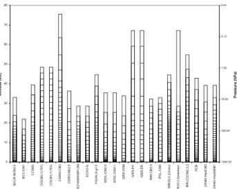
0 10 20 30 40 50 60 70 80 B C C R -B C M 2 .0 B C C -C M 1 C C S M 3 C G C M 3. 1( T 4 7) C G C M 3. 1( T 6 3) C N R M -C M 3 C S IR O -M k 3 .0 E C H A M 5 /M P I-O M E C H O -G F G O A L S -g 1 .0 G F D L -C M 2 .0 G F D L -C M 2 .1 G IS S -A O M G ISS-EH G ISS-ER IN M -C M 3 .0 IP S L -C M 4 M IR O C 3 .2 (h ir e s ) M IR O C 3 .2 (m e dr e s ) M R I-C G C M 2 .3 .2 PC M U K M O -H adC M 3 U K MO -H ad G E M1 A lti tu d e (k m ) 0.01 0.10 1.00 10.00 100.00 1000.00 Pr e s s u re ( h Pa )
Fig. 1. Approximate altitude of the vertical levels for models
sub-mitted to the IPCC AR4.
2) It has been shown that stratospheric variability and changes, particularly in the Northern and Southern Hemi-sphere polar vortices can affect the weather and climate of the troposphere (e.g., Shindell and Schmidt, 2004; Thomp-son et al., 2005). In particular ThompThomp-son et al. (2005) and Gillett and Thompson (2003) showed that part of the sur-face cooling in and around Antarctica could be associated with stratospheric ozone loss affecting the stratospheric po-lar vortex. In addition, several papers (e.g., Miller et al., 2006; Stenchikov et al., 2002) show that strong tropical vol-canic eruptions (e.g., Mt. Pinatubo) and ozone depletion can both affect the winter arctic oscillation in the Northern Hemi-sphere. However it also appears that a well resolved strato-sphere is required to accurately produce the correct tropo-spheric response (Gillett et al., 2002; Sigmond et al., 2004).
3) Several forcing or feedback mechanisms have a compo-nent associated with the stratosphere. Modeling the effects of stratospheric ozone depletion and explosive volcanic erup-tions have benefited from a better representation of the strato-sphere (Houghton et al., 2001). Solar irradiance changes may also have an effect on surface climate through inducing dy-namical changes in the stratosphere (Haigh, 2001; Haigh et al., 2005; Nathan and Cordero, 2006; Rind, 2002, 2004). It is also important to resolve stratospheric water vapor changes as these can have a large effect on surface climate, as well as in the stratosphere (e.g., Forster and Shine, 2002). For example Stuber et al. (2001) found that the ECHAM4 GCM had a very strong feedback associated with stratospheric wa-ter vapor increases resulting from tropopause temperature in-creases.
Pawson et al. (2000) designed an intercomparison to com-pare and characterize the stratosphere using GCMs from a variety of modeling groups. In this paper we repeat aspects of this intercomparison for the current IPCC AOGCMs which
were not specifically designed for stratospheric simulation. To aid climate-change attribution, we then expand this inter-comparison to look at temperature trends in the stratosphere simulated since 1958, and compare these to observations.
The primary goal of this paper is to evaluate the ability of the participating IPCC models to simulate the structure, variability and trends of the lower stratosphere during the 20th century. Understanding these strengths and weaknesses not only provides feedback to the modeling community, but can also communicate to the larger public the uncertainties of predictions for the 21st century. This work also aims to shed light on the potential for stratospheric change to af-fect temperatures in the upper troposphere, although this is not the focus of the paper. In Sect. 2, a brief description of the IPCC models and various observation-based datasets are given. Model simulations and their comparisons with obser-vations are given in Sect. 3, while Sect. 4 is devoted to un-derstanding the temperature trends in the stratosphere over the last three decades. Section 5 is a discussion regarding the vertical profile of temperature trends and we finish with our conclusions in Sect. 6.
2 Model and observed data
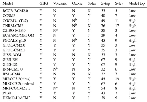
The analysis uses AOGCM simulations from the IPCC Model archive at the Program for Climate Model Diagno-sis and Intercomparison (PCMDI). Nineteen AOGCM sim-ulations submitted to the archive from groups in ten dif-ferent countries are compared using wind and temperature fields from the climate of the 20th century experiments. For each model, the run 1 simulation was used, even if multi-ple ensemble members were available. These models incor-porate various natural and anthropogenic forcings including changes in ozone distribution, greenhouse gases and aerosols distribution, although not all models incorporate all of these forcing mechanisms. A list of the model forcings directly relevant to the stratosphere is given in Table 1 and will be discussed further in the next section.
The submitted model simulations record data at 17 vertical levels in the atmosphere (1000, 925, 850, 700, 600, 500, 400, 300, 250, 200, 150, 100, 70, 50, 30, 20, 10 hPa). The actual model top and number and placement of stratospheric levels vary from model to model, and are shown in Fig. 1. While the majority of models do have a model top above 10 hPa, the number of levels above the tropopause and the vertical resolution varies widely. Of the 19 models, only eight have more than three levels above 10 hPa. This scarcity of model levels in the stratosphere may be a significant impairment to accurately resolving the large scale structure and variability of the stratosphere (Hamilton et al., 1999).
Observational climatologies of temperature are used from both satellite and radiosonde observations. These include data from the Microwave Sounding Unit (MSU) carried on the NOAA polar orbiting satellites. Retrievals from the MSU
Table 1. Specific forcings and details of the vertical model structure for each model submitted to the IPCC. The forcing terms are for the 20th
century simulation (20CM3) where GHG represent increases in well-mixed greenhouse gases, volcanic refers to volcanic aerosols, ozone refers to changes in stratospheric ozone and solar refers to changes in solar irradiance. The term Z-top refers to the approximate altitude of the top of the model, S-lev refers to the number of stratospheric levels. Models with a top at or above 45 km are classified as “High” while models with tops below that level are classified as “‘Low”.
Model GHG Volcanic Ozone Solar Z-top S-lev Model top
BCCR-BCM2.0 Y N N N 33 5 Low CCSM3 Y Y Y Y 40 7 Low CGCM3.1(T47) Y N Nb ? 49 11 High CNRM-CM3 Y N Nb N 76 17 High CSIRO-Mk3.0 Y Na Y N 38 3 Low ECHAM5/MPI-OM Y N Y ? 29 4 Low FGOALS-g1.0 Y N Nb Y 45 9 High GFDL-CM2.0 Y Y Y Y 35 3 Low GFDL-CM2.1 Y Y Y Y 35 3 Low GISS-AOM Y N N N 33 3 Low GISS-EH Y Y Y Y 67 9 High GISS-ER Y Y Y Y 67 9 High INM-CM3.0 Y Na N N 32 6 Low IPSL-CM4 Y N N N 32 7 Low MIROC3.2(hires) Y Y Y Y 45 19 High MIROC3.2(medres) Y Y Y Y 67 6 High MRI-CGCM2.3.2 Y Na N Y 54 8 High PCM Y Y Y Y 43 7 Low UKMO-HadCM3 Y N Y ? 39 5 Low
Na= Documentation claims inclusion of volcanic aerosols, but Fig. 6 shows no temperature response to volcanic eruptions. Nb= Documentation claims inclusion of ozone trends, but Fig. 7 shows little cooling in the lower stratosphere.
provide atmospheric temperature at broadly defined levels of the troposphere and lower stratosphere. In this study, we use a climatology of MSU temperature data compiled by Re-mote Sensing Systems (RSS, Mears et al., 2003) of channel 2 (MSU2) and channel 4 (MSU4) retrievals of monthly and zonally averaged gridded temperature anomalies between 1979-99.
We use two radiosonde datasets compiled from the groups at the Hadley Centre (HadAT2, Thorne et al., 2005) and the NOAA (RATPAC-A, Free et al., 2005). These datasets, which use subsets of the global radiosonde network and span the years 1958–2004, are compiled into monthly average temperature anomalies. While these recently developed ra-diosonde climatologies incorporate various adjustments to account for data inhomogeneities (Free et al., 2004), a re-cent analysis by Randel and Wu (2006) suggests a systematic cold bias in the RATPAC-A tropical lower stratospheric data compared to the MSU satellite observations. This potential cold bias in the tropical lower stratosphere radiosonde ob-servations will be considered in the subsequent model com-parisons. While uncertainties regarding the MSU and ra-diosonde observations exist, previous analyses suggest that these datasets are appropriate for the study of large scale atmospheric variations (Seidel et al., 2004). A further
dis-cussion of observational uncertainties will be provided in Sect. 5.
The model data will also be compared to the National Cen-ter for Environmental Prediction/National CenCen-ter for Atmo-spheric Research (hereafter NCEP) Reanalysis. The NCEP data are derived using atmospheric general circulation mod-els in a data assimilation system using in-situ and remotely sensed observations (Kistler et al., 2001). The NCEP re-analysis is available from 1948, but for stratospheric com-parisons, only since the beginning of satellite observations in 1979 are the data likely to be reliable for global strato-spheric studies (Randel et al., 2004). Although the ERA-40 reanalysis dataset has a higher range of altitudes, there are not significant differences between NCEP and ERA-40 in the stratosphere (Randel et al., 2004), and thus we will only show results using the NCEP reanalysis.
3 20th century climate: model intercomparison
The AOGCMs participating in the IPCC model comparison represent the most advanced and comprehensive set of cli-mate simulations so far produced. Simulations for the 20th century have been compared with each other and with avail-able observations. In Tavail-able 1, we identify a subset of
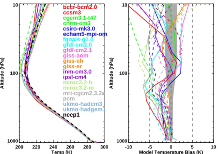
forc-200 220 240 260 280 300 Temp (K) 1000 100 10 Altitude (hPa) bccr-bcm2.0 ccsm3 cgcm3.1-t47 cnrm-cm3 csiro-mk3.0 echam5-mpi-om fgoals-g1.0 gfdl-cm2.0 gfdl-cm2.1 giss-aom giss-eh giss-er inm-cm3.0 ipsl-cm4 miroc3.2-h miroc3.2-m mri-cgcm2.3.2a pcm ukmo-hadcm3 ukmo-hadgem1 ncep1 ncep1 -10 -5 0 5 10
Model Temperature Bias (K) 1000
100 10
Altitude (hPa)
Fig. 2. Globally averaged temperature (left) and model
tempera-ture bias (right) between 1979–1999 for the climate models and the NCEP reanalysis. The lines identifying each model alternate be-tween solid and dashed, so that for each color the first listed model uses a solid line and the second listed model a dashed line. The gray shading in the model temperature bias plot shows NCEP plus and minus 2 standard deviations around the climatological mean.
ings used in the IPCC simulations of the 20th century climate that directly influence the stratosphere. The information on model forcing was largely obtained from the IPCC model website, where modeling groups supplied information about their runs. For model simulations where the supplied infor-mation did not appear to match the model temperature sim-ulations, a note was made. While all the models include the steady increase in greenhouse gas forcing, the models differ in their inclusion of variations in stratospheric ozone deple-tion, volcanic aerosols and variations in solar radiation. In the following section, an analysis of model experiments is made to assess model performance and the role of various forcing processes.
Figure 2 shows a vertical profile of the annual average global temperature from the IPCC models and the model temperature bias with respect to the NCEP reanalysis. The temperature distribution is averaged between 1979–1999 and ranges from the surface to 10 hPa. The temperature distri-bution illustrates the delineation in lapse rate between the troposphere and stratosphere, and the minimum in temper-ature at the tropopause. Near the surface and throughout the middle troposphere, the IPCC models agree reasonably well with each other and are generally within 2–3 K of the NCEP reanalysis, while at higher altitudes, the spread among the models increases. For example, at 700 hPa, the range of IPCC models differ by only ∼3 K, while at 200 hPa and 10 hPa, the models differ by 6 K and 17 K respectively. Both the NCEP standard deviation and the model bias compared to NCEP are larger in the stratosphere compared to the tropo-sphere. The models generally underestimate the global tem-perature in the stratosphere, a common GCM characteristic
-50 0 50 Latitude 200 220 240 260 280 300 Temp (K) bccr-bcm2.0 ccsm3 cgcm3.1-t47 cnrm-cm3 csiro-mk3.0 echam5-mpi-om fgoals-g1.0 gfdl-cm2.0 gfdl-cm2.1 giss-aom giss-eh giss-er inm-cm3.0 ipsl-cm4 miroc3.2-h miroc3.2-m mri-cgcm2.3.2a pcm ukmo-hadcm3 ukmo-hadgem1 ncep1 bccr-bcm2.0 ccsm3 cgcm3.1-t47 cnrm-cm3 csiro-mk3.0 echam5-mpi-om fgoals-g1.0 gfdl-cm2.0 gfdl-cm2.1 giss-aom giss-eh giss-er inm-cm3.0 ipsl-cm4 miroc3.2-h miroc3.2-m mri-cgcm2.3.2a pcm ukmo-hadcm3 ukmo-hadgem1 ncep1 σ
Fig. 3. Zonally and annually averaged temperature at 500 hPa
(up-per) and 50 hPa (lower) between 1979–1999 from the climate mod-els and NCEP. The 2-σ variation in the NCEP reanalysis is shown in the heavy black vertical lines, and the colors are as in Fig. 2.
observed in various model intercomparisons (e.g., Austin et al., 2003; Pawson et al., 2000), while there is also a clear cold bias observed in the middle and upper troposphere.
A comparison of zonally averaged temperatures averaged between 1979–1999 at 500 hPa and 50 hPa from the models and NCEP is displayed in Fig. 3. In the middle troposphere, the models are within 5 K of each other and the NCEP re-analysis, with the uncertainty in NCEP less than 5 K at all latitudes. At 500 hPa the largest difference between models and observations is seen at the polar NH, where the mod-els are consistently colder than NCEP. An evaluation of sea-sonal temperature variations (not shown) shows that during both December, January, February (DJF) and June, July, Au-gust (JJA), most models are cooler than NCEP in the NH, while in the SH, there does not appear a similar bias. In the stratosphere, the range of temperatures between models is larger than in the troposphere, with a spread in magnitude of about 11 K in the tropics and poles and a slightly smaller range at midlatitudes. As shown by the uncertainty in the NCEP reanalyses, the natural variability in the stratosphere and especially near the polar stratosphere is larger than in the troposphere.
At the poles, the models generally are in reasonable agree-ment with the NCEP analyses, with no apparent cold pole biases that was a feature of older versions of GCMs (e.g., Pawson et al., 2000). In fact, the corresponding winter (DJF) polar temperatures in the NH are almost all within the NCEP uncertainty, while in the SH, of the 11 models that are out-side the NCEP uncertainty, eight of the models are biased warm. In the tropics, a majority of the model simulations are cooler than the reanalysis, and the model to model variability is larger than in the extratropics, while the natural variability in the tropics is actually smaller than in the poles. Thus, the cooling bias seen in the global average temperature (Fig. 2),
70-90N: DJF
-15 -10 -5 0 5 10
Difference (model - NCEP) 1000 100 10 Pressure (hPa) 70-90N: DJF -15 -10 -5 0 5 10
Difference (model - NCEP) 1000 100 10 Pressure (hPa) 70-90S: JJA -15 -10 -5 0 5 10
Difference (model - NCEP) 1000 100 10 Pressure (hPa) 70-90S: JJA -15 -10 -5 0 5 10
Difference (model - NCEP) 1000
100 10
Pressure (hPa)
Fig. 4. Zonally averaged temperature difference in K between the
models and NCEP in the high latitude winter hemisphere averaged between 1979–1999. Models with a high top are averaged together and displayed with a solid line and models with a low top are aver-aged together and displayed with a dashed line. The differences are computed for DJF (left) and JJA (right). The gray shading indicates the 1 sigma standard deviation in the NCEP reanalysis.
at least at 50 hPa, is not from a cold pole bias, but rather from biases in the tropical latitudes. However, at higher al-titudes, a cold pole bias is seen in many models. For ex-ample at 10 hPa, during DJF, 14/19 of the models are colder than the observed variability between 70–90 N, while during JJA, 14/19 are colder than the observed variability between 70–90 S. These results imply that model representation of the planetary wave spectrum in the lower stratosphere of the win-ter hemisphere may be reasonable, while higher up this may not be the case. A natural question is then what role does the location of the model lid and number of stratospheric levels have on these results?
To evaluate the potential role of the vertical resolution and location of the model lid on the structure of stratospheric temperature, we group the models into two categories based on the altitude of the model lid and then examine the seasonal temperature variation between models and NCEP at three lat-itude ranges (70–90◦N, 30◦N–30◦S and 70–90◦S) during the winter of each hemisphere (Fig. 4). The first group is la-beled “high” and has a model lid at or above 45 km (∼2 hPa; indicated as high in Table 1) while the second group is la-beled “low” and has a model lid below 45 km. Figure 4 illus-trates the results of this comparison showing the difference (model – NCEP) for the two model groups in the high lati-tude winter hemisphere. During DJF and JJA, the difference between models with low and high tops is only significant near 10 hPa, the top reporting altitude for the IPCC dataset. In both cases, the models with a lower top (and fewer strato-spheric levels) have a cold bias at 10 hPa of nearly 15 K, while the higher top models have a corresponding cold bias of between 4–7 K. While there does not seem to be any sta-tistically significant bias at lower altitudes, it is clear that fur-ther analysis is required to more completely understand how the representation of the stratosphere affects atmospheric cir-culation at lower levels. It is certainly plausible that bi-ases at upper levels would alter wave-mean flow interaction, and thus affect circulation and structure at lower levels. We also note that in our analysis, we don’t find any systematic
May Dec June bccr-bcm2.0 May Dec June ccsm3 May Dec June cgcm3.1-t47 May Dec June cnrm-cm3 May Dec June csiro-mk3.0 May Dec June echam5-mpi-om May Dec June fgoals-g1.0 May Dec June gfdl-cm2.0 May Dec June giss-eh May Dec June inm-cm3.0 May Dec June ipsl-cm4 May Dec June miroc3.2-h May Dec June mri-cgcm2.3.2a May Dec June pcm May Dec June ukmo-hadcm3 May Dec
June NCEP Reanalysis
-20 0 20 40
Zonal wind (m/s) at 60N and 50hPa May Dec June Dec JuneJan bccr-bcm2.0 Dec JuneJan ccsm3 Dec JuneJan cgcm3.1-t47 Dec JuneJan cnrm-cm3 Dec
JuneJan csiro-mk3.0 Dec
JuneJan echam5-mpi-om Dec
JuneJan fgoals-g1.0 Dec
JuneJan gfdl-cm2.0 Dec
JuneJan giss-eh Dec
JuneJan inm-cm3.0 Dec
JuneJan ipsl-cm4 Dec
JuneJan miroc3.2-h Dec
JuneJan mri-cgcm2.3.2a Dec
JuneJan pcm
Dec
JuneJan ukmo-hadcm3 Dec
JuneJan NCEP Reanalysis
-20 0 20 40 60
Zonal wind (m/s) at 60S and 50hPa Dec
JuneJan
Fig. 5. Time series of zonally averaged zonal wind at 60◦N (left)
and 60◦S (right) at 50 hPa between the year 1979–1999 for a subset
of the submitted IPCC models and the NCEP reanalysis. Each of the 20 years of data is plotted on top of each other and compared to the 20 year mean NCEP reanalysis given in the black bold line.
temperature bias based on the inclusion of ozone depletion within these models.
The evolution of stratospheric winds is related to tempera-ture variations and ultimately controlled by large scale wave activity. In Fig. 5, the annual cycle in zonal wind at 60◦N and 60◦S at 50 hPa is displayed for each of the IPCC mod-els and the NCEP reanalysis for the years 1979–1999. In the NH, the winds are westerly and strongest during winter (DJF) and easterly and weak in the summer (JJA). By plot-ting each year on the same scale, the interannual variabil-ity can also be estimated. While overall there is reasonable agreement with NCEP in terms of the timing of the maxi-mum westerly winds, there exist significant variations in the peak magnitude of the westerly winds and the magnitude of the interannual variability. The interannual variability in NH DJF winds range from ∼6 m s−1in the CSIRO model to al-most 20 m s−1in the MRI model, compared to NCEP which is around ∼20 m s−1.
The variability in the SH is markedly different compared with the NH. The year to year variability of peak westerly winds ranges from 4–10 m s−1, almost half the variability seen in the NH. The smaller variability in the SH polar winds indicates a weaker planetary wave spectrum and is gener-ally consistent with observation (Newman and Nash, 2005). While the maximum winds reach over 50 m s−1in a couple of the models, the NCEP reanalysis maximum winds ap-pears larger than all the models except the CCSM3 model. However, because few reliable radiosonde observations in the middle to high latitude SH exist, biases in the NCEP re-analysis may exist at these locations (Randel et al., 2004). At higher altitudes, the magnitude of the winter winds increases in both hemispheres, as does the range of variability between models.
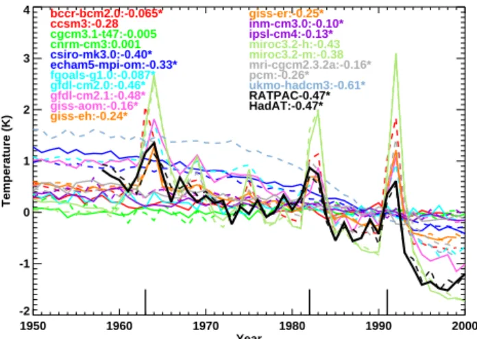
1950 1960 1970 1980 1990 2000 Year -2 -1 0 1 2 3 4 Temperature (K) bccr-bcm2.0:-0.065* ccsm3:-0.28 cgcm3.1-t47:-0.005 cnrm-cm3:0.001 csiro-mk3.0:-0.40* echam5-mpi-om:-0.33* fgoals-g1.0:-0.087* gfdl-cm2.0:-0.46* gfdl-cm2.1:-0.48* giss-aom:-0.16* giss-eh:-0.24* giss-er:-0.25* inm-cm3.0:-0.10* ipsl-cm4:-0.13* miroc3.2-h:-0.43 miroc3.2-m:-0.38 mri-cgcm2.3.2a:-0.16* pcm:-0.26* ukmo-hadcm3:-0.61* RATPAC-0.47* HadAT:-0.47*
Fig. 6. Time series of globally averaged annual temperature anomaly averaged at 50 hPa. The solid vertical black lines indi-cate major volcanic eruptions and the bold lines (solid and dashed) represent the radiosonde observations from RATPAC and HadAT respectively. Next to each model is the linear temperature trend in K decade−1calculated between 1958–1999, and the lines alternate
from solid to dashed as in Fig. 2. Models with statistically signifi-cant trends are indicated with asterisk (*) after the trend.
A comparison between zonal winds at 60◦N and 60◦S (Fig. 5) suggests that while hemispheric variations between the poles are reasonably captured, important departures from the observed climatology exist. This suggests that variations in dynamics and the characterization of large scale waves in IPCC models may inhibit the ability of models to accurately resolve stratospheric variability and change.
4 20th century trends
The primary radiative forcing mechanisms responsible for global temperature changes in the stratosphere over the last three decades have been increases in well-mixed GHG con-centrations, declines in stratospheric ozone, explosive vol-canic eruptions and solar changes (e.g., Ramaswamy et al., 2006). Increases in stratospheric water vapor may also in-fluence global temperature trends (e.g., Shine et al., 2003). As the future promises further changes in all of these forcing processes, temperatures in the stratosphere will continue to change.
Figure 6 shows a time series of global temperature anomaly at 50 hPa from the IPCC models and radiosonde observations between the years 1950 and 1999. Trends are determined from a linear regression, while a Student t-test is performed to determine if the trend is statistically significant. In cases where the trend is statistically significant at the 95% levels, an asterisk (*) is placed next to the trend.
Model temperatures at 50 hPa show that the majority of models indicate some cooling since 1958, with generally larger cooling rates since 1980. The cooling trend ranges
from −0.06 to −0.61 K decade−1 in models with statisti-cally significant trends, compared to the radiosonde obser-vations that both show a statistically significant cooling of
∼0.47 K decade−1. Among the models examined, 14 out
of 19 (12 out of 19) show a statistically significant cooling trend between 1958–1999 (1979–1999). However, among these models, the majority underestimate the observed ra-diosonde trend, with only four models (CSIRO-MK3.0; GFDL-CM2.1; UKMO-HADCM3) near or above the ra-diosonde trend. The two simulations by MIROC3.2h/m were also close to the observed trend, but were not statistically sig-nificant probably due to high variability caused by excessive sensitivity to volcanoes. As discussed below, the models that include ozone depletion forcing were much closer to obser-vations compared to models without ozone trends.
The most apparent feature in the 50 hPa temperature time series outside of the cooling trend are the three warm-ing perturbations correspondwarm-ing to the volcanic eruptions of Mt. Agung (1963), El Chich´on (1982) and Mt. Pinatubo (1991). The warming results from increases in the absorption of incoming solar radiation and the absorption of outgoing infrared radiation by volcanic aerosols (Ramaswamy et al., 2001). As indicated in the forcing table (Table 1), eight of the models used for the IPCC include volcanic perturbations, although it was reported that two other models also included volcanic perturbations and yet did not show any correspond-ing temperature response.
A simple analysis is performed to estimate the response in temperature due to the three large volcanic eruptions. The av-erage model temperature for the five years prior to the erup-tion is subtracted from the temperature one year following the eruption. In this way, we can compare the model response with the radiosonde observation.
The model warming associated with the Mt. Agung erup-tion in 1963 and El Chich´on in 1982 range from 0.5 K to 2.4 K compared to the radiosonde observations that warmed globally by between 0.4 K–0.6 K. The Mt. Pinatubo eruption produced a large temperature response observed in both ra-diosonde and satellites (Free and Angell, 2002; Karl et al., 2006) of about 1 K, while the models that include volcanic aerosols range from 1K to 3.5 K. The tendency of the mod-els to overestimate the volcanic induced warming is espe-cially large in a subset of the models. A comparison of the model and observed temperature response shows that about half the models that include volcanic aerosols (i.e., CCSM3, MIROC3.2 and PCM) overestimate the observed warming by a factor of 1.8–3.7. The excessive warming seen in MIROC3.2 has also been noted in Stenchikov et al. (2006). At higher altitudes (10 hPa; not shown), cooling trends are consistently larger and the magnitude of temperature variations associated with volcanic perturbations is reduced. Qualitatively, the trend toward stronger cooling with altitude generally agrees with the results of Shine et al. (2003) at 10 hPa and will be discussed further below.
-1.5 -1.0 -0.5 0.0 0.5 Trend (K/decade) 1000 100 10 Pressure HadAT RATPAC ukmo-hadcm3 pcm mri-cgcm2.3.2a miroc3.2-m miroc3.2-h ipsl-cm4 inm-cm3.0 giss-er giss-eh giss-aom gfdl-cm2.1 gfdl-cm2.0 fgoals-g1.0 echam5-mpi-om csiro-mk3.0 cnrm-cm3 cgcm3.1-t47 ccsm3 bccr-bcm2.0 HadAT RATPAC ukmo-hadcm3 pcm mri-cgcm2.3.2a miroc3.2-m miroc3.2-h ipsl-cm4 inm-cm3.0 giss-er giss-eh giss-aom gfdl-cm2.1 gfdl-cm2.0 fgoals-g1.0 echam5-mpi-om csiro-mk3.0 cnrm-cm3 cgcm3.1-t47 ccsm3 bccr-bcm2.0
Fig. 7. The vertical distributions of model average global
tempera-ture trends in K decade−1are calculated between 1958–1999. The
radiosonde observations are given by the star and diamond symbols, and the thin horizontal line corresponds to their 2-sigma variation.
Global model trends at altitudes from the surface to 10 hPa calculated between 1958–1999 are compared with the corre-sponding radiosonde observations in Fig. 7. The 2-sigma un-certainty in the HadAT2 and RATPAC-A radiosonde trends are computed using the standard error, while each measure-ment was assumed to be independent where autocorrelation has not been accounted for. The radiosonde trends, which are in good overall agreement with each other, show warm-ing within the troposphere between 0.1 to 0.2 K decade−1at the surface to between 0.1 to 0.3 K decade−1up to 250 hPa. Between 200 and 150 hPa, the crossover point between tro-pospheric warming and stratospheric cooling in both ra-diosonde observations are collocated, while there are large differences among the models. Above 100 hPa, atmospheric cooling increases with altitude up to about −0.5 K decade−1 at 50 hPa. Model predictions generally range from 0.05 to 0.2 K decade−1 at the surface to 0.1 to 0.3 K decade−1 at 250 hPa. In the upper levels, the range of model trends becomes wider, ranging from −0.6 to 0 K decade−1 at 50 hPa, compared to a radiosonde calculated trend of
−0.5 K decade−1. While the majority of models are within
the 2-sigma uncertainty of the radiosonde observations in the lower and middle troposphere (e.g., at 500 hPa, 16/19 mod-els are within the uncertainty), in the upper troposphere and lower stratosphere, the majority of models show not enough cooling and are outside the uncertainty (e.g., at 50 hPa, 4/19 models are within uncertainty). While a cooling bias in the temperature trends derived from radiosonde observa-tions may exist (e.g., Randel and Wu, 2006; Seidel et al., 2004), most models simulate the past stratospheric tempera-ture trends quite poorly.
A potential explanation for why some of the models used for the IPCC compare poorly to radiosonde temperature trends is the absence of stratospheric ozone depletion
(Ra--1.5 -1.0 -0.5 0.0 0.5 Trend (K/decade) 1000 100 10 Pressure (hPa) Avg Sonde No O3 Yes O3 -1.5 -1.0 -0.5 0.0 0.5 Trend (K/decade) 1000 100 10 Pressure (hPa) Sat - RSS Avg Sonde No O3 Yes O3
Fig. 8. The model average global temperature trend calculated
be-tween 1958–1999 (left) and 1979–1999 (right). The solid (dashed) lines represent trends averaged from models with (without) strato-spheric ozone depletion. Average radiosonde trends and their 2-sigma variation are given by the red stars and the thin horizontal lines respectively. In the 1979–1999 trend, the satellite observations are given by the triangle symbol, where the thin horizontal line rep-resents the 2-sigma variation in temperature and the thin vertical line represents the approximate vertical range of the observations.
maswamy et al., 2006; Shine et al., 2003). As illustrated in Table 1, of the 19 models that we compare for the 20th century, all models include well-mixed greenhouse gas forc-ing while only 11 include stratospheric ozone depletion. To explore this further, temperature trends for models with and without ozone depletion are compared in Fig. 8 for the two time periods of 1958–1999 and 1979–1999. The simulations are separated based on the inclusion of stratospheric ozone depletion and model temperature trends are averaged in these two groups. The temperature trends from the RATPAC-A and HadAT2 radiosonde observations are also averaged, and the 2-sigma estimate of the trend uncertainty is indicated us-ing horizontal lines. For the calculations of temperature trend between 1979–1999, satellite-derived trends computed from the RSS MSU analyses and their 2-sigma uncertainty are also shown, along with the approximate vertical range of these observations.
In the trend calculations for both time periods, the mod-els that include ozone depletion are significantly closer to the observations than the models that omit ozone vari-ations. In the trend between 1958–1999, the 50 hPa trend for the models with ozone depletion average almost
−0.4 K decade−1while the models without ozone depletion
are around −0.1 K decade−1. In this case, the models with ozone depletion are within the range of uncertainty for the radiosonde observations. In the lower stratosphere/upper tro-posphere near (150–100 hPa), even models with ozone deple-tion fall outside the uncertainty of radiosonde observadeple-tions, while below 150 hPa, the models with ozone depletion are
-1.5 -1.0 -0.5 0.0 0.5 Trend (K/decade) 1000 100 10 Pressure Sat - RSS Avg Sonde No O3 Yes O3
Fig. 9. As in Fig. 8 except for the tropical trend (30◦N–30◦S)
between 1979–1999 trend. Satellite observations are given by the triangle symbol, where the thin vertical line represents the 2-sigma uncertainty and the thin vertical line represents the approximate ver-tical range of the observations.
within the radiosonde uncertainty and the models without ozone depletion remain outside the observations all the way down to 700 hPa.
The crossover point between the tropospheric warming and stratospheric cooling is also significantly different be-tween the two model groups. The models with ozone de-pletion show a crossover point at around 150 hPa, while the models without ozone depletion show a crossover point at 70 hPa or about 4.8 km higher in altitude. From 200 hPa down to the surface, the models including ozone depletion are within the range of uncertainty for the radiosonde ob-servations, while the models without ozone depletion are warmer than the observations down to 500 hPa.
The global trends computed for the years 1979–1999 show a similar overall pattern compared to the 1958–1999 data, although the rate of the tropospheric warming and strato-spheric cooling is greater over the last two decades. The larger stratospheric cooling since 1979 is not surprising con-sidering most ozone depletion has occurred since 1979. In addition, the models also show better agreement to each other, and with both radiosonde and satellite observations from the surface to 300 hPa. At higher altitudes, how-ever, the spread between the two model groups is larger than during 1958–1999. At 50 hPa, the temperature trend is −0.6 K decade−1 for the models with ozone depletion and −0.1 K decade−1for the models without ozone deple-tion, while the radiosonde and satellite observations are
−0.8 K decade−1and −0.45 K decade−1respectively. These
results are qualitatively consistent with Shine et al. (2003) who found significant divergence in the magnitude of model derived vertical temperature trends even when the same ozone trend datasets were employed in different models. As discussed previously, it has been suggested that radiosonde trends in stratospheric cooling may be too large as a result of instrument biases at tropical latitudes (Randel et al., 2006). Indeed there is better agreement between the models and the satellite observations, although at 70 hPa, the models includ-ing ozone depletion are within the uncertainty of both obser-vational datasets.
Temperature trends in the tropics (30◦N–30◦S) calculated between 1979–1999 are shown in Fig. 9. From 50 hPa up to 10 hPa, the results look quite similar to the global model trends. The models that include stratospheric ozone de-pletion produce a larger cooling trend compared to models that do not. At these altitudes, the magnitude of the ra-diosonde trends is similar for the global and tropical aver-ages, although the 2-sigma uncertainty in the tropical trend is about 20% larger than the global value. In the lower strato-sphere and upper tropostrato-sphere, the models show larger warm-ing trends in the tropics compared with the global trends. At 150 hPa, the tropical trends with and without ozone de-pletion are between 0.1 and 0.2 K decade−1 more positive than the global trends. The crossover point between tropo-spheric warming and stratotropo-spheric cooling for the models in-cluding stratospheric ozone depletion is around 150 hPa for the global dataset and nearly 100 hPa for the tropical data. These changes are also reflected in the radiosonde observa-tions, where the crossover point is estimated at 250 hPa glob-ally and near 200 hPa in the tropics. Thompson and Solomon (2005) found similar vertical profiles of temperature trends over 1979–2003 using both NCEP reanalysis and radiosonde datasets.
Below 200 hPa, the models and both satellite and ra-diosonde observations show statistically similar magnitudes in tropical warming trends, although the models are system-atically warmer than the observations. The maximum warm-ing trend in the tropical troposphere occurs near 300 hPa at around 0.3 K decade−1, while the maximum warming trend in the global troposphere occurs near 200 hPa at around 0.2 K decade−1. The larger warming in the tropics compared to the extratropics has been observed in previous model in-tercomparisons (e.g., IPCC, 2001) and the larger warming in the free troposphere compared to the surface was also identi-fied in some observational trends and in the current group of IPCC models (Karl et al., 2006; Santer et al., 2005). The dif-ference between the average models with and without ozone depletion in the upper troposphere and lower stratosphere (200 hPa–50 hPa) is less in the tropics compared to the global trends.
This analysis illustrates the importance of including ozone variations for accurate calculations of trends in the lower stratosphere and upper troposphere. The significant differ-ence between the two groups of models suggests that
inclu-sion of ozone trends is critical to correctly modeling the long-term temperature variability in the stratosphere and may also be important to tropospheric climate. It is also noted that during the 1979–1999 period, two large volcanic eruptions produced large temperature perturbations and thus increased the uncertainty of the trend calculation during this period. Thus, the inclusion of volcanic aerosol is also important for assessing long-term climate variations in the stratosphere.
5 Discussion
Using MSU4 weighted temperature trends, Ramaswamy et al. (2006) recently attributed stratospheric temperature changes since 1979 to a combination of human and natu-ral factors. Good agreement between models and obser-vations were found when including well-mixed greenhouse gas changes, ozone changes and natural solar and volcanic changes. Each forcing contributed to the overall temperature-response time series. Their conclusions were based on results from a single model. Our findings generally support their conclusion across a wide range of models. However, our re-sults also suggest that ozone and volcanic forcings need to be carefully evaluated and implemented in models. In partic-ular, most models that included volcanic aerosols appear to have too much lower stratospheric (50 hPa) warming associ-ated with Mt Pinatubo.
For many years there has been controversy over appar-ent differences in modeled and observed temperature trends in the free troposphere, comparing trends from radioson-des, satellites and models (e.g., NRC, 2004). The recent Climate Change Science Program (CCSP) report (Karl et al., 2006) and the papers it cites (e.g., Fu et al., 2004) re-solve many of these issues. Our findings also tend to sup-port the conclusions of this resup-port, that models and observed trends appear in agreement, within their respective uncertain-ties. However, the CCSP report also notes that in the tropics “while almost all model simulations show greater warming aloft, most observations show greater warming at the sur-face”. Our results also support this conclusion. In particular they point to a real difference in the upper tropical tropo-sphere. Since 1979 there seems to have been a real cool-ing trend in the radiosonde observations down to altitudes around 200 hPa, whereas in models it is almost impossible to get a cooling below 100 hPa. They all exhibit a typical moist-adiabatic type of response (see e.g., Karl et al., 2006). Although the cooling trend in radiosonde datasets could be up to 0.1 K decade−1 too large in this region (Randel and Wu, 2006) and radiosonde trends have many uncertainties, this difference appears real.
Reasons for this difference could be associated with con-vection schemes in the models and/or their upper tropo-spheric water vapor feedback and/or resolution in the up-per troposphere. Much of the upup-per tropical troposphere (often termed the Tropical Tropopause Transition layer or
sub-stratosphere) is above typical altitudes of convective out-flow (e.g., Folkins et al., 1999; Gettelman and Forster, 2002; Thuburn and Craig, 2000) and as such may behave more like part of the stratosphere (Forster et al., 1997; Thuburn and Craig, 2000). Forster and Collins (2004) also suggest that although the water vapor feedback is generally well under-stood, the water vapor feedback in the upper troposphere may not be particularly well represented by model simulations of the Mt Pinatubo eruption. In the AOGCMs, relative humidity stays more or less constant with altitude (Karl et al., 2006). If this is not occurring in reality or if stratospheric radiative processes are playing more of a dominant role in the 200– 100 hPa region than the AOGCMs suggest, then temperature trends could be more negative than typical models suggest in this region. Randel et al. (2006) suggest that recent tempera-ture changes around the tropical tropopause could have been caused by a radiative response to a combination of ozone and water vapor changes; perhaps similar mechanisms are controlling the observed temperature trends in the 200 hPa– 100 hPa region and current AOGCMs are unable to capture these mechanisms. As the water vapor feedback from this region is very important for tropospheric climate evolution, our work suggests the need for a more focused effort to try and understand the large scale processes governing tempera-ture trends in the region, as well as efforts to make sure that AOGCMs can adequately simulate these responses.
6 Conclusions
AOGCM simulations submitted for the Fourth Assessment Report of the IPCC are analyzed to assess the ability of these models to simulate stratospheric variability and trends. Model temperature simulations are compared with NCEP re-analysis, and show that model to model variability is larger in the stratosphere compared to the troposphere, even when nat-ural variability is considered. Model simulations that include volcanic aerosols are necessary to reproduce the observed in-terannual variability in the stratosphere, although about half the models that include volcanic aerosols tend to significantly over predict the temperature response at 50 hPa. Although a cold temperature bias in relation to NCEP is seen in a major-ity of the models throughout the stratosphere, the presence of a cold pole bias is only evident at 10 hPa during the winter. At 50 hPa, most models are within the NCEP variability in the NH winter, and within or warmer than the NCEP vari-ability in the SH winter. However, at 10 hPa, about half the models are between 10–15 K colder than NCEP. It appears that this difference is related to representation of the strato-sphere within each model. In models with few stratospheric levels and a relatively low model top, the cold pole bias is about 9 K larger than the models with more stratospheric lev-els and a higher model top. This comparison suggests that in the present collection of models used by the IPCC, about half the models do not possess a high enough model top to
accurately simulate stratospheric variability at 10 hPa. This shortcoming is expected to affect other fields at 10 hPa and is likely to contribute to unrealistic variability at lower levels, although this has not been explicitly verified in this study and remains a topic of future study.
Stratospheric temperature trends in models are compared to existing radiosonde and satellite observed trends. In gen-eral, the models tend to underestimate the cooling trends in the stratosphere observed over the last forty years. The cool-ing of the stratosphere, which is largely controlled by de-clines in stratospheric ozone and increases in tropospheric GHGs, is only well simulated in models that include ozone depletion over the last thirty years. This agrees with previ-ous studies (i.e., Shine et al., 2003) that examined how tem-perature responds to ozone, GHG and water vapor changes using a middle atmosphere model. Our work, however, shows that the largest discrepancy between model trends and observations is found in the upper troposphere and lower stratosphere, where even models that include ozone deple-tion do not cool as much as the observadeple-tions. This discrep-ancy appears largest between 1979–1999, in tropical lati-tudes (30 N–30 S) between 100–200 hPa. Although tropical radiosonde observations may themselves possess a spurious cooling trend, our analysis suggests that these differences ap-pear real and should motivate further investigations to iden-tify the source of these differences.
Over the next century, we expect that stratospheric tem-peratures will continue to change. Simulations of the 21st century used for the IPCC AR4 (not shown) indicate that the stratosphere will continue to cool, although there is a wide range of projections. Model predictions show that the strength of cooling in the stratosphere is dependent on both the particular emission scenario, which indicates the level of greenhouse gas forcing, and the amount of stratospheric ozone. However, because of difficulties in obtaining infor-mation regarding the ozone distribution used in 21st cen-tury simulations, coupled with the wide variations in future ozone distributions between the models, a more detailed un-derstanding of how temperature will vary in the future is especially challenging with this dataset. This demonstrates how important experimental design and availability of meta-data can be in model intercomparisons.
As stratospheric temperatures and winds are also sensi-tive to variations in tropospheric wave processes, it is also important to investigate how gravity and larger scale wave processes are represented in models, and whether model bi-ases are introduced through the particular implementation of these processes. At present there remains significant uncer-tainty concerning dynamical processes associated with the parameterization of gravity waves and propagation of plane-tary waves in global models (e.g., Austin et al., 2003; Shep-herd and Shaw, 2004). With concurrent changes in ozone and GHGs, there is an important need to understand how changes in wave-mean flow interaction in the middle atmo-sphere may affect climate both in the stratoatmo-sphere and
tro-posphere (Cordero and Nathan, 2005; Nathan and Cordero, 2006), and to assess how these processes are represented in climate models.
Acknowledgements. We gratefully acknowledge the international modeling groups for providing their data for analysis, the Program for Climate Model Diagnosis and Intercomparison (PCMDI) for collecting and archiving the model data, the JSC/CLIVAR Working Group on Coupled Modeling (WGCM) and their Coupled Model Intercomparison Project (CMIP) and Climate Simulation Panel for organizing the model data analysis activity, and the IPCC WG1 TSU for technical support. The IPCC Data Archive at Lawrence Livermore National Laboratory is supported by the Office of Science, U.S. Department of Energy. ECC is supported by NSF’s Faculty Early Career Development Program (CAREER), Grant ATM-0449996 and NASA’s Living with a Star, Targeted Research and Technology Program, Grant LWS04-0025-0108. PMF is supported by a Roberts Research Fellowship.
Edited by: K. Hamilton
References
Austin, J. , Shindell, D., Beagley, S. R., Br¨uhl, C., Dameris, M., Manzini, E., Nagashima, T., Newman, P., Pawson, S., Pitari, G., Rozanov, E., Schnadt, C., and Shepherd, T. G.: Uncertainties and assessments of chemistry-climate models of the stratosphere, Atmos. Chem. Phys., 3, 1–27, 2003,
http://www.atmos-chem-phys.net/3/1/2003/.
Cordero, E. C. and Nathan, T .R.: A New Pathway for Commu-nicating the 11-Year Solar Cycle Signal to the QBO, Geophys. Res. Lett., 32, L18805, doi:10.1029/2005GL023696, 2005. Folkins, I., Lowewenstein, M., Podolske, J. R., Oltmans, S. J., and
Proffitt, M. H.: A barrier to vertical mixing at 14 km in the trop-ics: Evidence from ozonesondes and aircraft measurements, J. Geophys Res., 104, 22 095–22 102, 1999.
Forster, P. M. d. F., Blackburn, M., Glover, R., and Shine, K. P.: An examination of climate sensitivity for idealised climate experi-ments in an intermediate general circulation model, Clim. Dyn., 16, 833–849, 2000.
Forster, P. M. d. F. and Collins, M.: Quantifying the water vapour feedback associated with post-Pinatubo global cooling, Clim. Dyn., 23, 207–214, 2004.
Forster, P. M. d. F., Freckleton, R. S., and Shine, K. P.: On aspects of the concept of radiative forcing, Clim. Dyn., 13, 547–560, 1997. Forster, P. M. d. F. and Shine, K. P.: Assessing the climate impact and its uncertainty for trends in stratospheric water vapor, Geo-phys. Res. Lett., 29, 6, doi:1029/2001GL013909, 2002. Free, M. and Angell, J. K.: Effect of volcanoes on the vertical
tem-perature profile in radiosonde data, J. Geophys Res., 107(D10), 4101, doi:1029/2001JD001128, 2002.
Free, M., Angell, J. K., Durre, I., Lanzante, J. R., Peterson, T. C., and Seidel, D. J.: Using first differences to reduce inhomogeneity in radiosonde temperature datasets, J. Climate, 17, 4171–4179, 2004.
Free, M., Seidel, D. J., Angell, J. K., Lanzante, J., Durre, I., and Peterson, T. C.: Radiosonde atmospheric temperature prod-ucts for assessing climate (RATPAC): a new dataset of
large-area anomaly time series, J. Geophys Res., 110, D22101, doi:10.1029/2005JD006169, 2005.
Fu, Q., Johanson, C. M., Warren, S. G., and Seidel, D. J.: Contri-bution of stratospheric cooling to satellite-inferred tropospheric temperature trends, Nature, 429, 55–58, 2004.
Gettelman, A. and Forster, P. M. d. F.: Definition and climatology of the tropical tropopause layer, J. Meteor. Soc. Japan, 80, 911–924, 2002.
Gillett, N. P., Allen, M. R., McDonald, R. E., Senior, C. A., Shin-dell, D. T., and Schmidt, G. A.: How linear is the Arctic Oscilla-tion response to greenhouse gases?, J. Geophys Res., 107, 4022, doi:10.1029/2001JD000589, 2002.
Gillett, N. P. and Thompson, D. W.: Simulation of recent southern hemisphere climate change, Science, 302, 273–275, 2003. Haigh, J. D.: Climate variability and the influence of the sun,
Sci-ence, 294, 2109–2111, 2001.
Haigh, J. D., Blackburn, M., and Day, R.: The response of tropo-spheric circulation to perturbations in lower stratotropo-spheric tem-perature, J. Climate, 18, 3672–3691, 2005.
Hamilton, K., Wilson, R. J., and Hemler, R. S.: Middle atmosphere simulated with high vertical and horizontal resolution versions of a GCM: Improvements in the cold pole bias and generation of a QBO-like oscillation in the tropics, Atmos. Sci., 56, 3829–3846, 1999.
Houghton, J. T., Ding, Y., Griggs, D. J., Noguer, M., van der Linden, P. J., Dai, X., Maskell, K., and Johanson, C. A.: Climate Change 2001: the Scientific Basis, Cambridge University Press, 892 pp., 2001.
IPCC: Climate Change 2001: The Scientific Basis. Contribution of Working Group I to the Third Assessment Report of the Inter-governmental Panel on Climate Change, Cambridge University Press, Cambridge, UK, 881 pp., 2001.
Karl, T. R., Hassol, S. J., Miller, C. D., and Murray, W. L. (Eds.): Temperature Trends in the Lower Atmosphere: Steps for Under-standing and Reconciling Differences, The climate change sci-ence program and the subcommittee on global change research, Washington, D.C., USA, 2006.
Kistler, R., Kalnay, E., Collins, W., Saha, S., White, G., Woollen, J., Chelliah, M., Ebisuzaki, W., Kanamitsu, M., Kousky, V., Van der Dool, H., Jenne, R., and Fiorino, M.: The NCEP-NCAR 50-year reanalysis: Monthly means CD-ROM and documentation, Bull. Am. Met. Soc., 82, 247–267, 2001.
Mears, C. A., Schabel, M. C., and Wentz, F. J.: A reanalysis of the MSU channel 2 tropospheric temperature record, J. Climate, 16, 3650–3664, 2003.
Miller, R. L., Schmidt, G. A., and Shindell, D. T.: Forced annu-lar variations in the 20th century Intergovernmental Panel on Climate Change Fourth Assessment Report models, J. Geophys. Res., 111, D18101, doi:10.1029/2005JD006323, 2006.
Nathan, T. R. and Cordero, E. C.: An ozone-modified refractive in-dex for vertically propagating planetary waves, J. Geophys. Res., in press, 2006.
Newman, P. A. and Nash, E. R.: The unusual southern hemisphere stratosphere winter of 2002, J. Atmos. Sci., 62, 614–628, 2005. NRC: Climate data records from environmental satellites, National
Academy Press, 136 pp., 2004.
Pawson, S., Kodera, K., Hamilton, K., et al.: The GCM-Reality intercomparison project for SPARC (GRIPS): Scientific issues and initial results, Bull. Amer. Meteor. Soc., 81, 781–796, 2000.
Ramaswamy, V., Chanin, M.-L., Angell, J., Barnett, J., Gaffen, D. J., Gelman, M., Keckhut, P., Koshelkov, Y., Labitzke, K., Lin, J.-J. R., O’Neill, A., Nash, J., Randel, W., Rood, R., Shine, K., Shiotani, M., and Swinbank, R.: Stratospheric temperature trends: observations and models simulations, Rev. Geophys., 39, 71–122, doi:1999RG000065, 2001.
Ramaswamy, V., Schwarzkopf, M. D., Randel, W., Santer, B. D., Soden, B., and Stenchikov, G.: Anthropogenic and natural in-fluences in the evolution of lower stratospheric cooling, Science, 311, 1138–1141, 2006.
Randel, W., Udelhofen, P., Fleming, E. L., Geller, M. A., Gelman, M., Hamilton, K., Karoly, D. J., Ortland, D. A., Pawson, S., Swinbank, R., Wu, F., Baldwin, M. P., Chanin, M.-L., Keckhut, P., Labitzke, K., Remsberg, E., Simmons, A. J., and Wu, D.: The SPARC Intercomparison of middle-atmosphere climatologies, J. Climate, 17, 986–1003, 2004.
Randel, W. J. and Wu, F.: Biases in stratospheric and troposheric temperature trends derived from historical radiosonde data, J. Climate, 19(10), 2094–2104, 2006.
Randel, W. J., Wu, F., V¨omel, H., Nedoluha, H. G., and Forster, P. M. d. F.: Decreases in stratospheric water vapor since 2001: Links to changes in the tropical tropopause and the Brewer-Dobson circulation, J. Geophys Res., 111, D12312, doi:10.1029/2005JD006744, 2006.
Rind, D.: Climatology: The sun’s role in climate variations, Sci-ence, 296, 673–677, 2002.
Rind, D., Shindell, D., Perlwhitz, J., and Lerner, J.: The Rela-tive Importance of Solar and Anthropogenic Forcing of Climate Change between the Maunder Minimum and the Present, J. Cli-mate, 17, 906–929, 2004.
Santer, B. D., Sausen, R., Wigley, T. M. L., Boyle, J. S., AchutaRao, K., Doutriaux, C., Hansen, J. E., Meehl, G. A., Roeckner, E., Ruedy, R., Schmidt, G. A., and Taylor, K. E.: Behavior of tropopause height and atmospheric temperature in models, re-analyses and observations: Decadal changes, J. Geophys Res., 108, D14002, doi:10.1029/2002JD002258, 2003a.
Santer, B. D., Wehner, M. F., Wigley, T. M. L., Sausen, R., Meehl, G. A., Taylor, K. E., Ammann, C., Arblaster, J., Washington, W. M., Boyle, J. S., and Bruggemann, W.: Contributions of anthro-pogenic and natural forcing to recent tropopause height changes, Science, 301, 479–483, 2003b.
Santer, B. D., Wigley, T. M. L., Mears, C., Wentz, F. J., Klein, S. A., Seidel, D. J., Taylor, K. E., Thorne, P. W., Wehner, M. F., Gleck-ler, P. J., Boyle, J. S., Collins, W. D., Dixon, K. W., Doutriaux, C., Free, M., Fu, Q., Hansen, J. E., Jones, G. S., Ruedy, R., Karl, T. R., Lanzante, J. R., Meehl, G. A., Ramaswamy, V., Russell, G., and Schmidt, G. A.: Amplification of surface temperature trends and variability in the tropical atmosphere, Science, 309, 1551–1556, doi:10.1126/science.1114867, 2005.
Seidel, D. J., Angell, J. K., Christy, J., Free, M., Klein, S. A., Lan-zante, J. R., Mears, C., Parker, D. E., Schabel, M., Spencer, R., Sterin, A., Thorne, P. W., and Wentz, F. J.: Uncertainty in sig-nals of large-scale climate variations in radiosonde and satellite upper-air temperature datasets, J. Climate, 17, 2225–2240, 2004. Shepherd, T. G. and Shaw, T. A.: The angular momentum constraint on climate sensitivity and downward influence in the middle at-mosphere, J. Atmos. Sci., 61, 2899–2908, 2004.
Shindell, D. T. and Schmidt, G. A.: Southern hemisphere climate response to ozone changes and greenhouse gas increases,
Geo-phys. Res. Lett., 31, L18209, doi:10.1029/2004GL020724, 2004. Shine, K. P., Bourqui, M. S., Forster, P. M. F., et al.: A comparison of model-simulated trends in stratospheric temperature, Q. J. R. Met. Soc., 129, 1565–1588, doi:10.1256/qj.02.186, 2003. Sigmond, M., Siegmund, P. C., Manzini, E., and Kelder, H.: A
sim-ulation of the separate climate effects of middle-atmosphere and tropospheric CO2doubling, J. Climate, 17, 2352–2367, 2004.
Stenchikov, G., Hamiliton, K., Stouffer, R. J., Robock, A., Ra-maswamy, V., Santer, B. D., and Graf, H.-F.: Arctic oscillation response to volcanic eruptions in the IPCC AR4 climate mod-els, J. Geophys. Res., 111, D07107, doi:10.1029/2005JD006286, 2006.
Stenchikov, G., Robock, A., Ramaswamy, V., Schwarzkopf, M. D., Hamiliton, K., and Ramachandran, S.: Arctic oscillation re-sponse to the 1991 Mount Pinatubo eruption: effects of volcanic aerosols and ozone depletion, J. Geophys Res., 107(D24), 4803, doi:10.1029/2002JD002090, 2002.
Stuber, N., Ponater, M., and Sausen, R.: Is the climate sensitivity to ozone perturbations enhanced by stratospheric water vapor feed-back, Geophys. Res. Lett., 28, 2887–2890, 2001.
Tett, S. F. B., Mitchell, J. F. B., Parker, D. H., and Allen, M. R.: Hu-man influence on the atmospheric vertical temperature structure: Detection and observations, Science, 274, 1170–1173, 1996. Thompson, D. W., Baldwin, M. P., and Solomon, S.:
Stratosphere-troposphere coupling in the Southern Hemisphere, J. Atmos. Sci., 62, 708–715, 2005.
Thompson, D. W. and Solomon, S.: Recent stratospheric climate trends as evidenced in radiosonde data:Global structure and tro-pospheric linkages, J. Climate, 18, 4785–4795, 2005.
Thorne, P. W., Parker, D. E., Tett, S. F. B., Jones, P. D., McCarthy, M., Coleman, H., and Brohan, P.: Revisiting radiosonde upper air temperature from 1958 to 2002, J. Geophys. Res., 110, D18105, doi:10.1029/2004JD005753, 2005.
Thuburn, J. and Craig, G. C.: Stratospheric influence on tropopause height: The radiative constraint, J. Atmos. Sci., 57, 17–28, 2000. WMO: Scientific assessment of ozone depletion:2002. Global ozone research and monitoring project, Report number 47, 498, 2003.