HAL Id: hal-00295407
https://hal.archives-ouvertes.fr/hal-00295407
Submitted on 17 Mar 2004
HAL is a multi-disciplinary open access
archive for the deposit and dissemination of
sci-entific research documents, whether they are
pub-lished or not. The documents may come from
teaching and research institutions in France or
abroad, or from public or private research centers.
L’archive ouverte pluridisciplinaire HAL, est
destinée au dépôt et à la diffusion de documents
scientifiques de niveau recherche, publiés ou non,
émanant des établissements d’enseignement et de
recherche français ou étrangers, des laboratoires
publics ou privés.
Effects of various meteorological conditions and spatial
emissionresolutions on the ozone concentration and
ROG/NOx limitationin the Milan area (I)
N. Baertsch-Ritter, J. Keller, J. Dommen, A. S. H. Prevot
To cite this version:
N. Baertsch-Ritter, J. Keller, J. Dommen, A. S. H. Prevot. Effects of various meteorological conditions
and spatial emissionresolutions on the ozone concentration and ROG/NOx limitationin the Milan area
(I). Atmospheric Chemistry and Physics, European Geosciences Union, 2004, 4 (2), pp.423-438.
�hal-00295407�
www.atmos-chem-phys.org/acp/4/423/
SRef-ID: 1680-7324/acp/2004-4-423
Chemistry
and Physics
Effects of various meteorological conditions and spatial emission
resolutions on the ozone concentration and ROG/NO
x
limitation in
the Milan area (I)
N. Baertsch-Ritter, J. Keller, J. Dommen, and A. S. H. Prevot
Paul Scherrer Institute, Laboratory of Atmospheric Chemistry, CH-5232 Villigen PSI, Switzerland Received: 23 December 2002 – Published in Atmos. Chem. Phys. Discuss.: 12 February 2003 Revised: 24 February 2004 – Accepted: 24 February 2004 – Published: 17 March 2004
Abstract. The three-dimensional photochemical model
UAM-V is used to investigate the effects of various meteo-rological conditions and of the coarseness of emission inven-tories on the ozone concentration and ROG/NOxlimitation of the ozone production in the Po Basin in the northern part of Italy. As a base case, the high ozone episode with up to 200 ppb on 13 May 1998 was modelled and previously thor-oughly evaluated with measurements gained during a large field experiment. Systematic variations in meteorology are applied to mixing height, air temperature, specific humidity and wind speed. Three coarser emission inventories are ob-tained by resampling from 3×3 km2up to 54×54 km2 emis-sion grids. The model results show that changes in meteoro-logical input files strongly influence ozone in this area. For instance, temperature changes peak ozone by 10.1 ppb/◦C
and the ozone concentrations in Milan by 2.8 ppb/◦C. The
net ozone formation in northern Italy is more strongly tem-perature than humidity dependent, while the humidity is very important for the ROG/NOxlimitation of the ozone produc-tion. For all meteorological changes (e.g. doubling the mix-ing height), the modelled peak ozone remains ROG limited. A strong change towards NOxsensitivity in the ROG limited areas is only found if much coarser emission inventories were applied. Increasing ROG limited areas with increasing wind speed are found, because the ROG limited ozone chemistry induced by point sources is spread over a larger area. Simula-tions without point sources tend to increase the NOxlimited areas.
Correspondence to: A. S. H. Prevot
(andre.prevot@psi.ch)
1 Introduction
In the troposphere, ozone is formed through various chem-ical reactions involving NOx(NO+NO2=NOx), reactive or-ganic gases (ROG) and sunlight with non-linear dependen-cies (Lin et al., 1988; Sillman, 1999). Ozone formation is very sensitive to meteorological conditions as well as to pre-cursor emissions (NOxand ROG) (Br¨onnimann et al., 2002; Br¨onnimann and Neu, 1997; Wolff et al., 2001).
In Europe and the US, several studies have been performed analysing the impact of meteorological factors on measured ozone (Bloomfield et al., 1996; Davis et al., 1998) or sim-ulated ozone concentrations (Sillman and Samson, 1995; Khalid and Samson, 1996; Br¨onnimann and Neu, 1997). Dif-ferent authors used photochemical models and/or analysed the effects with the help of statistical analyses (Andreani-Aksoyoglu and Keller, 1996; Sistla et al., 1996; Porter et al., 2001). Other model studies showed the effect of the emission on the ozone formation using different grid sizes (Jang et al., 1995; Li et al., 1998). But hardly any information can be found about the dependence of the ROG and NOxsensitivity of the ozone production on meteorological variability.
The major errors in photochemical modelling evolve from unrealistic input of the meteorology and emissions (Russel and Dennis, 2000). The quality of the input files should be considered after a careful evaluation of the model results with regard to a wide range of measurements. Sometimes, only modelled ozone concentrations are compared to measure-ments and may simply agree by accident. It is well known, that different ROG/NOxratios may lead to the same ozone production. As a consequence, even if ozone is modelled cor-rectly, the model might propose ozone control strategies that are not adequate. But also unrealistic meteorological input parameters could alter the prediction of ozone and possibly the limitation of the ozone production.
During the PIPAPO field experiment (Pianura Padana Pro-duzione di Ozono) (Neftel et al., 2002) within the LOOP
424 N. Baertsch-Ritter et al.: Effects of various meteorological conditions and spatial emission resolutions (Limitation of Oxidant Production) project, a distinct ozone
episode near Milan, Italy with concentrations above 180 ppb on 13 May 1998 was studied by measurements on many platforms and several chemical transport models. Baertsch-Ritter et al. (2003) used the UAM-v (Urban Airshed Model with variable grid) to analyze this pollution episode. Within that study, the original emission inventory was modified based on the analysis of measurements of carbon monoxide, nitrogen oxides and reactive organic gases (Dommen et al., 2003). After the modification, no hydrogen peroxide peak was modeled anymore in the air masses including the peak ozone concentrations, as found in the measurements. Sill-man (1995) emphasized that the hydrogen peroxide produc-tion is very sensitive to NOxor ROG limited ozone produc-tion condiproduc-tions. The model run including the modificaproduc-tion of the emissions was used as the base case for this study.
One major question, that is addressed in this work, is how robust the model results are concerning the limitation of the ozone production. Downwind of Milan within the peak ozone area, very distinct ROG limited conditions were found (Baertsch-Ritter et al., 2003). The idea is now to systemati-cally change meteorological parameters and study how the ozone concentrations and the limitation of the ozone pro-duction is changing in the area around Milan. The range of these systematic variations do not reflect uncertainties of the meteorological model during that day but reflect condi-tions that could occur on different days in that area. Besides the influence of meteorological parameters, including mix-ing heights, air temperatures, specific humidities and wind speeds, the influence of coarser emission inventories is stud-ied by resampling the emissions of this area into coarser grids. Several point sources are included in the model sim-ulations affecting the modelling domain particularly. This paper may contribute to a better understanding how meteo-rological parameters and spatial resolution of the emission inventories influence ozone production and its limitation.
2 Area of investigation
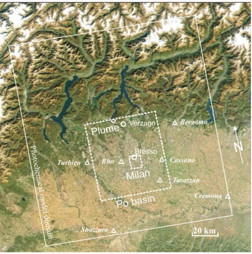
The area of investigation – the western part of the Po basin, Italy including parts of the Alps - is given as an extract of a true-colour MODIS image (http://modis.gsfc.nasa.gov), which was acquired from data collected on 11 October 2001 (Fig. 1). In the southern part of the scene the flat “Po Basin” with the city of Milan and the surrounding suburbs are partially visible. Roughly 9 million people are living in this large, densely populated and highly industrialized urban area. The Po Basin is rather flat, with an average altitude of 100 m a.s.l. To the north of Milan, the altitude increases, reaching the Alpine foothills (in the vicinity of the lakes, dark black areas) and the Alps in the most northern part of the satellite scene. The latter surpass over 3000 m a.s.l, around 150 km from Milan and are covered by snow and ice (white areas). Seven large point sources, mainly power stations and
refineries, are marked by triangles, which are treated explic-itly in the model simulations. At Bresso and Verzago, two well equipped supersites were operating during the field cam-paign. On Fig. 1, also the photochemical model domain and the areas used for statistical investigations are indicated.
3 Model description
System Application International (SAI) developed a three-dimensional photochemical model referred as Urban Airshed
Model with variable grid (UAM-V). The UAM-V
incorpo-rates two-way, horizontal and vertical multiple grid nest-ing, a plume-in-grid treatment of elevated point source emis-sions, dry deposition and three-dimensional meteorological input data (SAI, 1999). The model allows the description of regional-scale processes, simulating the effects of emissions, diffusion, advection, chemical transformation and surface re-moval processes. The chemistry is described by the Carbon Bond Mechanism IV (CBM-IV), which includes 94 chemi-cal reactions (Gery et al., 1989). The reaction rate constants in the model were updated based on Atkinson et al., 1997. In the original model version 1.15, an incorrect formulation of the transport schemes was detected. The model was then improved (Keller et al., 2002), which now is used in this pre-sented model study.
The meteorology of the base case was calculated with the meteorological pre-processor SAIMM (SAI Mesoscale Model, (SAI, 1995)). This model comes along with the UAM-V package and includes a set of utility programs for input preparation and data conversion between the meteoro-logical and chemical model. SAIMM was run with 19 layers and an extended domain (243 km×264 km) to limit the influ-ences at the boundaries of the modelling domain. The me-teorological pre-processor provides five meme-teorological in-put files that UAM-v requires (wind speed, temperature, wa-ter vapour, vertical turbulent exchange coefficient (kv)and
height/pressure).
The meteorological mesoscale model package is based on the hydrostatic model MM2 (Pielke, 1974). SAIMM is a prognostic model but includes four-dimensional data assim-ilation using observed temperature, moisture and wind data. The model employs the Newtonian relaxation or “nudging” technique in which one or more of the time-dependent vari-ables are relaxed or ”nudged” toward observed values that are spatially weighted during the course of the simulation (SAI, 1995). Thus, this technique provides more realistic meteoro-logical fields for use in air-quality modelling.
The meteorological simulation for the base case was done from 9–13 May. For the initialization and the four-dimensional data assimilation, hourly surface data were taken from the monitoring network ANETZ operated by Me-teo Swiss and from several ground stations operated dur-ing the PIPAPO field experiment (for details see Baertsch-Ritter et al., 2003). Information about upper air levels were
Bresso Rho Cassano
20 km
Bergamo Turbigo Snazzaro Tavazzan Cremona Photochemical model domain VerzagoN
Po basin
Milan
Plume
Fig. 1. Photochemical model domain in the northern part of Italy. Circles indicate Milan centre and the urban station Bresso. Triangles
denote point sources. The smaller square represents the area of “Milan” centre including station Bresso. The dotted circle denotes the core of the modelled ozone “Plume” of the Cases A–D, F and G at 15 h CET. The bigger square is denoted as “Po Basin” including the area of Milan and the core of the ozone plume. Different concentrations in the core of the ozone plume and means within the squares are calculated and compiled in Table 1.
available every 6 hours from balloon soundings at Linate air-port and every hour from a wind profiler in Seregno, 15km north of Milan. The model was “nudged” towards these ob-served values. Realistic surface wind fields with 2–3 m/s in the Po Basin were reproduced by SAIMM, whereas the mixing layer height was overestimated. From airplane mea-surements it is known that the mixing layer on 13 May was about 1100–1200 m a.s.l. Thus, the mixing layer height was restricted to the top of the fourth model layer (1000 m agl) by adjusting the vertical profile of the vertical turbulent ex-change coefficients (Baertsch-Ritter et al., 2003).
3.1 Model domain
The photochemical model simulations were performed in the so-called LOOP domain with a 3 km×3 km resolution. The west-east and north-south extension of the domain is 141 km and 162 km, respectively (Fig. 1). Eight vertical terrain fol-lowing atmospheric layers were used extending from the
sur-face up to 3000 m agl. The layers mid-points are found at 25, 100, 325, 750, 1250, 1750, 2250 and 2750 m agl.
3.2 Meteorological situation
The synoptic situation during the episode in May 1998 was favourable for high photooxidant production: clear sky, stag-nant weather condition, high irradiance and temperatures which were governed by a stationary high-pressure ridge at 500 hPa extending from north Africa to southern Scandi-navia. Daily temperatures in Milan exceeded 30◦C on 12 and
13 May. In the late afternoon of the second day, high convec-tive clouds developed in the mountains leading to thunder-storms and terminating the nice weather period. In the base case (bc), the maximum mixing height during daytime was between 1100 and 1200 m agl. Near the ground, the air tem-perature (T) at Milan centre at 15 h CET was around 29◦C with a specific humidity (q) of 8.2 g/kg, which corresponds to about 32% relative humidity. The pollution episode on
426 N. Baertsch-Ritter et al.: Effects of various meteorological conditions and spatial emission resolutions
Table 1. Compilation of mean O3concentration in the areas Milan, Plume and Po Basin (Fig. 1) for the variations of the Cases A–G valid for
13 May 1998 at 15 h CET. For the Cases B, C, and D, only the base case and the extreme variation results are shown. In additon, the mean average ozone concentrations are given for the model runs including 35% NOxand 35% anthropogenic ROG emission reduction respectively.
O3 O3 ( -35% ROG) O3 ( -35% NOx)
Variation
Milan Plume Po Basin Milan Plume Po Basin Milan Plume Po Basin
Mixing height (m a.g.l.)
A2 2000 93.0 134.4 101.8 91.5 112.2 97.5 96.5 129.5 102.5 A1 1500 101.1 168.7 109.8 99.4 129.1 104.9 104.1 159.5 109.7 bc 1000 115.5 195.0 118.4 113.0 133.7 112.4 118.2 196.1 118.5 ∆T (oC) B1 10 141.9 285.3 144.7 137.6 190.8 134.5 144.5 263.3 143.7 bc 0 115.5 195.0 118.4 113.0 133.7 112.4 118.2 196.1 118.5 B7 -4 103.9 162.0 107.1 101.9 112.6 102.4 106.8 175.8 108.0 ∆q (%) C1 20% 115.4 200.7 118.8 113.1 138.1 112.9 117.8 194.7 118.3 bc 0 115.5 195.0 118.4 113.0 133.7 112.4 118.2 196.1 118.5 C8 -60% 114.0 177.2 115.6 111.0 119.3 109.1 118.7 200.0 118.4 ∆T (oC), ∆q (%) D1 10, +110% 142.5 290.2 147.3 138.6 231.2 138.8 143.5 256.1 143.1 bc 0, 0% 115.5 195.0 118.4 113.0 133.7 112.4 118.2 196.1 118.5
Wind speed (enhancement)
bc * 1 115.5 195.0 118.4 113.0 133.7 112.4 118.2 196.1 118.5
E1 * 2 108.1 164.8 116.2 106.7 135.6 112.5 112.8 152.2 116.8
E2 * 5 105.6 127.2 111.3 104.6 116.3 109.4 110.8 133.1 112.6
Spatial resolution of the emission inventory (km2) (emissions including point sources)
bc 3 x 3 115.5 195.0 118.4 113.0 133.7 112.4 118.2 196.1 118.5
F1 9 x 9 118.5 192.3 119.9 116.1 133.1 113.7 120.1 192.5 119.6
F2 27 x 27 125.3 182.1 124.1 121.8 137.7 116.6 126.2 175.3 122.5
F3 54 x 54 142.1 156.8 128.7 136.9 143.5 123.2 136.1 143.7 123.5
Spatial resolution of the emission inventory (km2) (emissions without point sources)
bc 3 x 3 115.4 197.8 117.6 112.9 135.7 112.1 118.2 191.3 116.5
G1 9 x 9 118.5 194.1 119.3 116.1 135.1 113.5 120.1 187.7 117.6
G2 27 x 27 125.2 182.9 123.8 121.7 140.3 116.9 126.2 169.9 120.5
G3 54 x 54 142.0 152.6 128.0 136.9 143.1 123.7 136.1 136.9 121.1
13 May 1998 occurred under relatively dry conditions. The wind speed (v) in the Po Basin during daytime was around 2–3 m/s.
4 Design of various meteorological conditions
The base case for this study was taken from Baertsch-Ritter et al. (2003) that included a modification of original emis-sions. The idea here is to look at the influences of meteo-rological parameters individually. Five major “cases” were designed: Variations of the mixing heights (A), air tempera-tures (B) and specific humidities (C), combinations of Cases B and C (D) and enhancements of the wind speed (E). De-tailed information about the five cases are given in Table 1.
Within one case, different systematic variations were sim-ulated. The range of variations are mostly within the variabil-ity that can occur in this region on days with conditions that favour high ozone production. Only the very high tempera-tures are beyond regularly observed conditions. The three-dimensional meteorological fields were scaled as a whole, maintaining the vertical and horizontal differences. To in-crease the temperature by 2◦C as an example, the original three-dimensional temperature field of the bc was changed by adding 2◦C in each grid cell. The daily maximum of the original mixing height, 1000 m agl, was increased twice by 500 m. This was achieved by letting the vertical exchange coefficient drop to low levels at the top of the 5th or the 6th model level respectively. This is not a straight-forward method but probably one of the only ways to study the effects
of changes in mixing height individually without changing other parameters. The well-mixed boundary layer in A1 has now an extension of around 1500 m and in A2 of 2000 m.
In variations B1–B7, the original temperature field was varied with a 1T of −4, −2, 2, 4, 6, 8, 10◦C and in vari-ations D1–D5 with 1T of 2, 4, 6, 8, 10◦C. The undertaken variations of the original specific humidity field in variations C1–C8 are −60, −50, −40, −30, −20, −10, 10, 20% and in variations D1–D5 20, 45, 65, 90 and 110%. In variations D1–D5, the temperature enhancement was combined with a humidity increase. This is more representative for the real variations although also very dry and warm conditions can occur when northerly foehn winds are prevailing. For the D variations, the humidity was increased maximally without exceeding 95% relative humidity during night. At 15 h CET, the relative humidity for these variations is still low at Mi-lan with around 34 to 38%. In Table 1, only results of the extreme variations of the Cases B, C, and D are shown.
The preparation of the meteorological fields for variations E1–E2 was performed with SAIMM, assuring mass conser-vation. This means, that mass conservation in the meteo-rological model satisfies some discrete form of the continu-ity equation, which otherwise could lead to an inconsistency with the air quality model. In SAIMM, all available wind in-put information were enhanced for every simulated day until 12 h CET by a factor of 2 or 5 and used during the “nudging”. The resulting meteorological input files from SAIMM were used for the model simulations. As already found for the base case, the resulting wind speeds in the region of Milan were very similar as the given wind profiler measurements which are the most representative information for the whole mixing layer.
5 Design of various spatially coarser emission
invento-ries
The emission inventory compiled in the CBM-IV mechanism was modified corresponding to measurements during the PI-PAPO campaign (Dommen et al., 2003) and is used here for the base case. It contains 4 inorganic (NO, NO2, CO, SO2) and 12 ROG species (HCHO, ALD2, PAR, OLE, ETH, TOL, CRES, XYL, ISOP, MEOH, ETOH and METH) (Gery et al., 1989). All presented simulations are run on the basis of a 3 km×3 km grid size resolution of the emission inventory.
The resampling of the emission inventory to a spatially coarser inventory was performed in a simple way. The cho-sen resampling sizes of the new emission inventories are 9×9 km2, 27×27 km2and 54×54 km2, common multiples of the original grid size (Table 1, Cases F and G). At the eastern and the northern edge of the domain, the grid cells had to be reduced (e.g. 33×54 km2instead of 54×54 km2)in order to fit into the original domain. But this did not affect the re-distribution of the most important emissions around Milan. The emission inventory was resampled over the new chosen
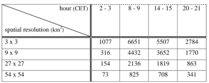
Table 2. Variation of the maximum NO emission (g/h) in Milan for
selected hours and different spatial resolutions of the used modified emission inventory. Milan hour (CET) spatial resolution (km2) 2 - 3 8 - 9 14 - 15 20 - 21 3 x 3 1077 6651 5507 2784 9 x 9 316 4432 3652 1770 27 x 27 154 2136 1819 863 54 x 54 73 825 708 341
sizes and the corresponding means were redistributed back into new emission inventory files with the original grid size. Retaining the original grid size resolution required no recal-culation of the meteorological input files and leads to no loss of details, as is reported by Kumar et al. (1994). In this way, the effect of the coarser emissions on the modelled concen-trations in the domain can be studied isolated. The meteorol-ogy at a coarser grid would lead to an additional modification of the modelled concentrations.
The applied up-scaling technique obviously reduces the emission variability of the highest emission grid cells in the city with the surrounding grid cells. The variations of the highest NO emission grid cell for Milan at different hours are given in Table 2. During one of the busy morning rush hours (8–9 h CET) the NO emission drops to 33%, 68% and to 87% of the original maximum emission when enlarging the spatial resolution of the emissions to 9×9 km2, 27×27 km2and to 54×54 km2, respectively.
In the variations of Case F (as in the Cases A–D), the point sources were treated explicitly. The design of the variations G1–G3, where no point sources are implemented during the model simulations, is used to investigate the influence of ex-plicitly treated point sources in different coarser inventory model runs.
6 Results and discussion
The results of the base case and the comparison with mea-surements are documented in Baertsch-Ritter et al. (2003). As can also be found in Table 1, ozone reached concentra-tions of 195 ppb. At the same time NOyconcentrations of 46 ppb were found. The ozone concentrations were highest near Verzago and the production of ozone was strongly ROG limited downwind of Milan and slightly NOxlimited in the surroundings (Fig. 2). Within 73.6% of the model grids in the Po basin (Fig. 1), the ozone production was ROG limited, in 20.3% NOxlimited (Table 5).
In addition to each simulation including the variation of individual meteorological parameters, ROG or NOx reduc-tion scenarios were modelled for each of these variareduc-tions. In
428 N. Baertsch-Ritter et al.: Effects of various meteorological conditions and spatial emission resolutions
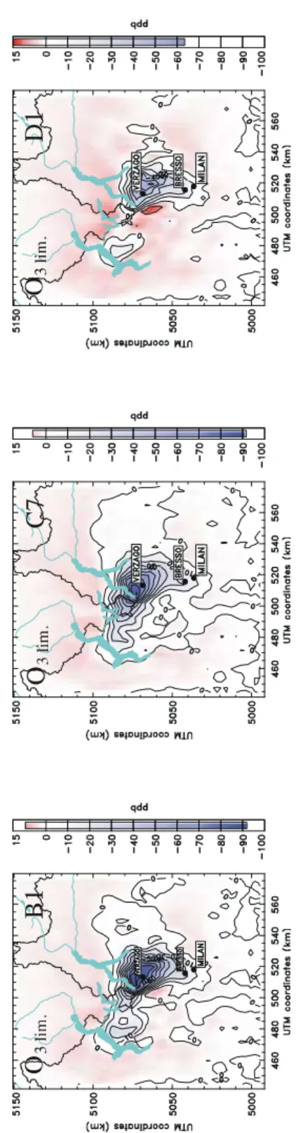
Fig. 2. Modelled ozone concentration and limitation for base case (bc) and selected variations given at 15 h CET. Variations G2 and G3 are
modelled without point sources.
these scenarios, anthropogenic ROG or NOxemissions were individually reduced by 35%. The difference of the ozone concentration for two such model runs yields the ozone lim-itation (O3lim., see definition below). The presented model
results are discussed for 13 May 1998 at 15 h CET. At this day, the highest photooxidant production was observed dur-ing the measurdur-ing campaign. This day and time of day can-not be regarded as generally representative for this region but
Fig. 2. Continued.
it is a good example for a very distinct ozone episode near Milan. Similar episodes were previously discussed (Prevot et al., 1997).
In order to quantify the model response on the mete-orological variations, averages were calculated for “Mi-lan” (81 km2), the “Po basin” (3969 km2)and the “Plume”
(9 km2)which includes the highest modelled ozone concen-trations. In Case E, the plume corresponding to the high-est concentration is not at the same spot. These regions are shown in Fig. 1 confined by dotted lines. Table 1 includes av-erage concentration of O3and the O3of both reduction sce-narios for all the Plume, Milan and the Po basin. In
Baertsch-430 N. Baertsch-Ritter et al.: Effects of various meteorological conditions and spatial emission resolutions
Table 3. Calculated slopes (ppb ozone/◦C temperature) from mea-surements and from model results for Cases B (temperature varia-tions) and D (temperature and humidity variavaria-tions) at different sites. Please see text for further explanation.
Model Measurements Regression Plume Milan Mendrisio Milan
Slopes case B 10.1 2.8 10 5.8
r2 0.99 0.99 0.6 0.44
Slopes case D 10.8 2.7
r2 0.99 0.99
Ritter et al. (2002) averages of hydrogen peroxide, NOyand NOxare provided and discussed in detail.
The following sections as well as most figures relate to the numbers in Table 1 and give some details about how the dif-ferent variations influence ozone and the limitation of ozone in this region. The quantification of the ROG and NOx reduc-tions on the ozone limitation of the different cases (Fig. 2) is expressed as
O3lim.=O3(−35%ROGanthrop.)−O3(−35%NOx)
NOx limited : O3lim.>0 ppb; ROGlimited : O3lim.<0 ppb Higher O3lim. refers to higher NOxsensitivity and lower O3lim.to higher ROG sensitivity in the modelling domain. Case A: mixing height
Figure 3a shows the influence of the enhanced mixing height on the modelled ozone concentration in the Po basin, Milan and the Plume. The changes lead to a significant decrease of the ozone concentration, especially in peak ozone. At 15 h CET, the modelled peak ozone drops from 195 ppb to 134 ppb (−31%), −19.5% in Milan and −14% in the Po basin when increasing the mixing height from 1000 to 2000 m agl. This means that even in Milan, where titration of ozone by NO plays an important role, ozone is reduced when the primary emissions are diluted into a larger volume. Taking the whole domain into account, the percentage of NOxlimited grid cells increased by around 3% (Fig. 4). This seems to be very small but a relative change of 1% indicates 25 grid cells or 228 km2. Nevertheless it is clear that the production of ozone downwind of Milan remains strongly ROG limited even with a doubling of the mixing height (Fig. 2).
Case B: temperature
At constant specific humidity, the modelled ozone pro-duction at the given time is almost linearly dependent on the temperature (solid lines in Fig. 3b). The linear regression coefficients of the temperature dependence of the modelled
ozone concentrations of Case B at 15 h CET are given in Ta-ble 3. In Milan a slope of 2.8 ppb/◦C is found. The strongest
gradient is found in the ozone plume with 10.1 ppb/◦C. As
a result, the ozone production efficiency with increasing temperature is about 3.6 times higher in the Plume than in Milan, which reflects mostly the inflow conditions south of Milan.
Generally, higher temperatures alter the chemical reaction rates. These higher temperatures are related to an enhanced decomposition of peroxyacetylnitrate (PAN) and higher ho-mologues (Sillman et al., 1990; Sillman and Samson, 1995; Vogel et al., 1999; Wunderli and Gehrig, 1991). The equilib-rium between NO2and PAN (and its homologues) is shifted to higher NO2concentrations at higher temperatures. With increasing temperature of Case B, the net formation of PAN in the modelling domain is reduced and is most pronounced in the ozone plume. In bc, the modelled PAN concentra-tion at 15 h CET is 13.1 ppb, while the concentraconcentra-tion in B1 decreases to 6.4 ppb. The change in PAN production is the most important reason for the enhanced ozone production at higher temperatures as found in a sensitivity study changing only the reaction rates involving PAN. If PAN is formed less, more radicals are available to react with NO to form NO2 which produces ozone. In the NOxsensitive production, also the higher NOxconcentrations favour higher ozone produc-tion.
The number of ROG limited grid cells strongly increases (by around 25%) comparing B1 with bc (Fig. 4). The more strongly NOxlimited areas (O3lim.>5 ppb) decrease from 94 grid cells (bc) to only 15 grid cells in variation B1. Hence, the modelling domain tends to get less NOxlimited with in-creasing temperature (Fig. 2).
In reality, increasing air temperature also leads to in-creased biogenic emissions in reality. Dommen et al. (2002) derived from measurements especially for the Po Basin near Milan a low contribution (∼6%) of biogenic emissions to the ROG reactivity. The biogenic emission contribution to the ROG reactivity in the modelled ozone plume is also low (∼4.7%). For this reason, the changes in biogenic emissions are not expected to strongly alter the effect on the limitation in Case B, which otherwise would foster NOxlimitation.
Different calculated slopes in Cases B and D (same as Case B, but with strongly increased humidity amount) are compared with slopes determined from longer-term mea-surements in Milan and Mendrisio. The latter monitoring site is found about 18 km northwest of Verzago and is similarly frequently as Verzago affected by polluted air masses stemming from Milan. Weber et al. (2002) analyzed the daily ozone maximum in Mendrisio and correlated them with temperatures. If one defines days with (ozone maximum) – (ozone concentration at noon) >40 ppb as plume days, one finds 10 ppb ozone/◦C for temperatures between 20 and 30◦C. The value of 40 ppb is arbitrary, but seems to be a reasonable limit for the differentiation. Analyzing the ozone concentration found in the PIPAPO
1000 1500 2000
Mixing height (m a.g.l.) 80 100 120 140 160 180 200 O z one ( ppb) 24 28 32 36 40 Temperature (oC) 100 120 140 160 180 200 220 240 260 280 300 O z o ne ( p pb) (a) (b) 2 4 6 8 Specific humidity (g/kg) 10 100 120 140 160 180 200 O z on e ( ppb) * 1 * 2 * 5
Wind speed (enhancement) 100 120 140 160 180 200 O z one ( ppb) (c) (d) 3 x 3 9 x 9 27 x 27 54 x 54 3 x 3 9 x 9 27 x 27 54 x 54 Spatial resolution of the emission inventory (km2)
100 120 140 160 180 200 O z one ( p p b ) (e)
Fig. 3. Peak ozone (triangles) and mean ozone concentrations in the areas of Milan (crosses) and Po Basin (stars) for the Cases A–G. Figure 3b
includes Cases B (temperature variations, solid lines) and D (temperature and humidity variations, dashed lines). Cases F (variations of the spatial resolution of the emission inventory including point sources, solid lines) and G (ditto, but without point sources) are compiled in Fig. 3e.
database for Milan for ozone concentrations >60 ppb and temperatures between 20 and 30◦C results in a slope of 5.8 ppb/◦C (Table 3). Usually with increasing temperature the background ozone concentration will also change in re-ality. This fact is not taken into account in the model, where the boundary conditions remain the same for all simulations. Especially the calculated slope in the model for Milan would
therefore be higher because the ozone background is a much higher fraction of the ozone concentration in Milan than in the ozone plume. The calculated slopes in Case D are very similar to Case B, indicating that the strong humidity increase has a minor effect on the dependence of the ozone concentration on temperature.
432 N. Baertsch-Ritter et al.: Effects of various meteorological conditions and spatial emission resolutions
1000 1500 2000
Mixing height (m a.g.l.) 0 20 40 60 80 100 Rel a ti ve n u m b e r of g rid c e lls (% ) (a) (b) -4 -2 0 2 4 6 8 1 ∆ Temperature to bc (oC) 0 20 40 60 80 100 R e la ti v e num be r of gr id c e lls ( % ) 0 -60 -50 -40 -30 -20 -10 0 10 20 ∆ Specific humidity to bc (%) 0 20 40 60 80 100 R e la ti ve n u m b e r o f g rid ce lls (%) (c) (d) (f) 3 x 3 9 x 9 27 x 27 54 x 54 Spatial resolution of the emission inventory (km2)
0 20 40 60 80 100 R e la ti ve n u mb er o f gr id ce lls ( % ) 0, 0 2, +20 4, +45 6, +65 8, +90 10, +110 ∆ Temperature to bc (oC), ∆ Specific humidity to bc (%) 0 20 40 60 80 100 Re la ti v e nu m ber of gr id c e ll s ( % ) * 1 * 2 * 5
Wind speed (enhancement) 0 20 40 60 80 100 R e lati ve nu mbe r o f grid cel ls (%) (e)
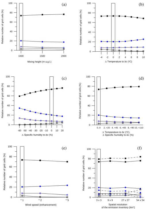
Fig. 4. Fraction of NOx(filled squares) and ROG (filled circles) limited grid cells in whole modelling domain for Cases A–G. Unfilled
symbols indicate NOxsensitive grid cells O3lim.>5 ppb and ROG sensitive grid cells O3lim.<−5 ppb. Cases F (variations of the spatial
resolution of the emission inventory including point sources, solid lines) and G (variations of the spatial resolution of the emission inventory without point sources, dashed lines) are compiled in f).
Case C: specific humidity
Figure 3c shows that in Milan, the Po basin and the Plume ozone is slightly increasing (maximum 1.2%, 2.7% and 13% respectively) with increasing humidity. As the humidity is one of the factors controlling OH production, a positive correlation can be expected. However especially in Milan and in the Po basin the influence of the water vapour on the ozone concentration is rather weak.
In Fig. 4c, the number of ROG sensitive grid cells O3lim.<0 ppb shows a strong increase with decreasing hu-midity. This related to generally higher NOxconcentrations in the modelling domain because of slower formation of ni-tric acid. The ROG sensitive grid cells O3lim.<−5 ppb in-crease as well strongly, while the fraction of NOxlimited grid cells O3lim.>5 ppb in the base case drop from around 3% to 0.2% in variation C7. The last number indicates that the do-main gets very weak NOxlimited for the benefit of stronger
ROG limited areas. Figure 2 shows the limitation of C7. Vogel et al. (1999) studied in a box model the influence of humidity on the ozone production and transition value of NOy. In their work, a humidity change from 3.1 to 9.3 g/kg shifted the transition of maximum ozone concentration from 20 ppb to 30 ppb NOy. Below these levels, ozone increased with decreasing humidity and above, ozone increased with increasing humidity. The latter condition is similar to the behaviour of the ozone and NOyconcentrations of Case C in the two areas and the ozone plume of the modelling domain. In the NOx limited areas, ozone increases with decreasing humidity. Note, that the humidity enhancement in this case covers a comparable humidity range as described by (Vogel et al., 1999).
Case D: temperature and specific humidity
The variations in Case D are represented by a combi-nation of altered temperatures and water contents of the input files. As is denoted in Sect. 4, the specific humidity supplements in the input files was calculated based on the varied temperatures ensuring that 95% relative humidity was not exceeded during night. The temperature enhancements in Cases B and D are the same, whereas the total amount of humidity in D is strongly increased compared to Case C. The observed effects of the latter case on the ozone concentration in the two areas and the ozone plume are included in Fig. 3b (dashed lines), allowing to compare the results directly with Case B. Even with the increased formation rate of OH, only a small additional incline of the ozone formation is found – in the urban area it is hardly noticeable.
The number of NOx limited grid cells in the modelling domain is enhanced by 5.8% comparing bc and variation D1. The ratio of all ROG limited grids decrease correspondingly, as well as the number of the O3lim.<−5 ppb ROG grid cells. In Fig. 2, the modelled limitation of the variation D1 is given. It clearly shows that the NOx limited areas are in-creased compared to B1. North of the point source of Tur-bigo, the ROG sensitive area influenced by this point source is now isolated and not merged any more with the ROG sen-sitive urban plume area.
Concluding from the model results of the individual temperature (Case B) and humidity variations (Case C) com-pared to the combined variations in Case D, the net ozone formation in northern Italy is more strongly temperature than humidity dependent. Higher temperature yields rather more ROG sensitive conditions, while increased humidity is leading to more NOxsensitivity. In our combined Case D, the effect of humidity is stronger yielding more NOxlimited conditions in spite of higher temperatures.
Case E: wind speed
The preparation of the input file for the model simula-tions with regard to enhanced wind speeds is described in
Sect. 4. Assuming that the formation of the plume takes place during the stagnant morning hours by accumulation of primary pollutants, enhanced wind speeds before 12 h CET was chosen to provoke a greater dilution of primary pollu-tants in the modelling domain. The primary emissions in Milan in the morning hours are distributed over a greater area and are further transported to the west of Milan city before the ozone plume turns north to the Alps reaching peak ozone at somewhat different locations than in the base case. In variation E2, no distinct ozone plume is formed, rather two areas with enhanced O3 concentrations (not shown), whereas peak ozone is reached at 17 h CET. The changes in ozone concentration in Milan and “Po Basin” are lower than 10 ppb comparing bc with E2, while the ozone plume indicate a change of around 70 ppb. As a result, the ozone concentration in the whole modelling domain gets more evenly distributed and in addition gets more dominated by the boundary conditions with increased wind speeds.
In Fig. 4e, the number of all NOx (O3lim.>0 ppb) and ROG (O3lim.<0 ppb) limited grid cells of Case E are given. Enhanced wind speeds change the ROG limited areas from 20.3% to 24% comparing bc with E2. The corresponding NOxlimited areas change from 73.6% to 69.9%. Moreover, both NOxsensitive (O3lim.>5 ppb) and ROG sensitive areas (O3lim.<−5 ppb) strongly decrease.
Analyzing the limitations without point sources reveals an interesting feature. The ROG and NOxlimited areas for this base case are 79.1% and 14.7%, respectively (Fig. 4f). Simu-lating E1 without point sources results now in a total number of NOxand ROG limited grid cells of 84.8% and 15.2%, re-spectively, pointing to an increased number of NOxlimited grid cells! Hence, the point sources demonstrate a strong ROG sensitive influence on the modelling domain. Conclud-ing, the treatment of point sources in model simulations can reverse the dependence of the ROG/NOxlimitation on wind speed changes.
In these model simulations, enhanced wind speeds are indicative of greater dilution of polluted plumes as found by Biswas and Rao (2001). Sillman et al. (1995) report 10% change in simulated peak O3and 15% change in concurrent NOy concentration associated with enhanced wind speeds. Our model leads to a 15% reduction in peak ozone and 41% NOywhen doubling the morning wind speeds.
Cases F and G: Enlarging the spatial resolution of the emission inventory
Enlarging the spatial resolution of the emission inven-tory reduces the emission variability because highest emission grid cells are averaged with surrounding grid cells. The simple applied resampling technique of the original emission inventory is described in Sect. 5. An example of the highest NO emission variation in Milan with respect to the changed spatial resolution is also given there (Table 2). The lower emission strength in the city emission grid cells
434 N. Baertsch-Ritter et al.: Effects of various meteorological conditions and spatial emission resolutions leads to a reduced ozone formation in the Plume (Fig. 3e,
solid line). In Milan and in the Po basin, a gradual increase of the ozone concentration with coarser emission inventory is found. The modelled ozone distribution for variation F1 (9×9 km2)is almost not discernible from bc, which is shown in Fig. 2.
The mean ozone concentration of Case G – basically Case F without point sources – is included in Fig. 3e (dashed lines) and compared to Case F. The impact of point sources in the Milan, Po basin area and Plume is small (<4 ppb). However, local ozone destruction of >−30 ppb and >−10 ppb is found where the point sources of Tavazzan and Turbigo influence the modelling domain.
Reducing the spatial resolution leads to an enhanced num-ber of NOxlimited grid cells in the model (Fig. 4f). Cases F and G are both included in Fig. 4f, showing the differences when excluding the point sources in the model simulations. The number of the NOxlimited grid cells change from bc to variation F1 by 2.2% to 75.8% and from bc to variation G3 by 4.9% to 84%, where the greatest changes occur again be-tween 27 x 27 km2and 54×54 km2. No ROG O3lim.<−5 ppb grids are found in variation G3 (54×54 km2).
In Fig. 2, the ozone concentrations and the calculated limitations for the grid resolution of 27×27 km2 (Case F) and 54×54 km2 (Case G) are given. The use of a coarser emission inventory not only enhances the num-ber of NOx limited grid cells but obviously also leads to a less detailed resolution of observed features. Maxi-mum O3lim.>0 ppb hardly changes when applying a coarser emission inventory: It remains between about 8–10 ppb. However, the maximum O3 lim.<0 ppb tends to get much smaller (G2 (O3lim.=−36 ppb)) nearly reaching 0 ppb (G3 (O3 lim.=−1.3 ppb)). In variation F3, the visible ROG limited areas are only due to the ozone plumes of the point sources.
The features in the ozone and O3 lim.distributions are still well reproduced at a resolution of 9 km×9 km, but at the higher resolution, very drastically at 54 km×54 km, the fea-tures are strongly altered.
Kumar et al. (1994) applied a multiscale air quality model with three different grid resolutions (5×5 km2, 10×10 km2 and 20×20 km2)on southern California. Thunis (2001) used the three dimensional Eulerian TAPOM (Transport and Air Pollution Model) in the Po Basin for the same time period in 1998. He applied a comparable emission inventory to the not modified original emission inventory used in Baertsch-Ritter et al. (2002) and reduced the spatial resolution from 4×4 km2 to 10×10 km2and 50×50 km2. In both works of Kumar et al. (1994) and Thunis (2001), a uniform enlarging of the spa-tial resolution of the emission inventory yielded higher levels of urban ozone, similar to our findings. The latter author also reports reduced peak ozone due to coarser emission inven-tories. However, his base case does not compare with other model simulations (Martilli et al., 2002; Baertsch-Ritter et al., 2003).
Concluding, coarser grid sizes lead not only to different ozone concentrations but also to influences on the limita-tion, which obviously may lead to incorrect control strate-gies. Hence, the grid size of a chosen modelling domain should be carefully evaluated.
7 Summary
The three-dimensional photochemical model UAM-V is used to investigate the effects of various meteorological conditions and different spatial emission resolutions on the ozone con-centration and ROG/NOx limitation in the Milan region in the northern part of Italy during the intensive measuring cam-paigns of PIPAPO. The quantification of ROG and NOx re-ductions on the ozone limitation is described in Sect. 4.6.
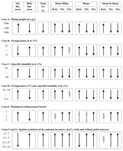
Seven Cases A–G are designed, for which the input files of the base case (bc) were varied. The results of the variations in two defined areas (Milan and “Po Basin”) and the ozone plume – expressed as tendency of increasing NOx or ROG limited areas, increasing ozone, H2O2, NO2 and NOy concentrations – are given as a summary in Table 4. The arrows do not take the power of the tendency into account. More quantitative results and discussion on the meteorological influences on hydrogen peroxide, NOy, and NOxcan be found in Baertsch-Ritter (2002). Table 5 shows for selected variations the quantification of the NOx and ROG limited areas. Most of the undertaken variations lay within possible meteorological conditions that could occur from spring to autumn. The main findings of all cases concerning the limitation are:
Case A: An increase of the mixing height leads to a slight increase of NOxlimited areas in the whole modelling domain, but no dramatic change in the limitation in the various areas is observed.
Case B: The ROG limited areas increase with higher tem-peratures, mostly because of lower PAN formation at higher temperatures.
Case C: Increased humidity leads to strongly increased NOx limited areas.
Case D: Higher temperature yields rather more ROG limited conditions, while increased humidity leads to NOx limita-tion. In this case, the effect of humidity is stronger yielding more NOxlimited areas in spite of higher temperatures. Case E: With increasing wind speed, emissions get more evenly distributed in the whole modelling area and gets more influenced by the boundary conditions. Increasing ROG limited areas with increasing wind speed are found, while simulations without point sources tend to increase NOx limited areas. Hence, the treatment of point sources in model simulations can reverse the dependence of the ROG/NOxlimitation on wind speed changes.
Cases F and G: The NOxlimited areas increase with coarser emissions. Excluding point sources in the model simulations
Table 4. The results of Cases A–G are expressed as tendency of increasing NOxor ROG limited areas in the Milan, Plume and Po Basin.
Note, that the power of the tendency is not taken into account.
Mean Milan Plume Mean Po Basin
NOx lim. areas ROG lim. areas Peak O3, O3 H2O2 NOx NOy H2O2 NOx NOy H2O2 NOx NOy
Case A: Mixing height (m a.g.l.)
2000 1500 1000 Case B: ∆Temperature to bc (oC) 10 … -4
Case C: ∆Specific humidity to bc (%)
20
…
- 60
Case D: ∆Temperature (oC) and ∆specific humidity to bc (%)
10, 110
…
0, 0
Case E: Windspeed (enhancement factor)
1 2
5
Cases F and G: Spatial resolution of the emission inventory (km2), (with and without point sources)
3 x 3 9 x 9 27 x 27 54 x 54 ~ equal ~ equal not e v id ent ~ equal not ev id en t ~ e q u al ~ equal
lead to stronger increased NOxlimited areas than with point sources.
The model results show that changes in meteorological in-put files have the largest effect on peak ozone. The tempera-ture dependence on the ozone formation in the model results and in measurements was compared. In the modelled ozone plume and in Milan, slopes of 10.1 ppb ozone/◦C and 2.8 ppb ozone/◦C were found, whereas slopes of 10 ppb ozone/◦C and 5.8 ppb ozone/◦C were found in measurements.
In-creased background concentrations with increasing temper-atures were not taken into account in the model simulations, possibly explaining the difference between model and mea-surements.
The net ozone formation in northern Italy is more strongly temperature than humidity dependent, while the humidity is very important for the ROG/NOxformation of the ozone
pro-duction. The calculated slopes in Case D are very similar to Case B, also indicating that the strong humidity increase has a minor effect on the dependence of the ozone concentration on temperature.
For each of the meteorological variations (e.g. doubling the mixing height), the modelled ozone plume remains ROG limited on 13 May. A strong change towards NOx sensitiv-ity in the ROG limited areas was only found if much coarser emission inventories were applied. It is advisable to perform model simulations in the Po Basin with a spatial grid resolu-tion better than 10×10 km2. The influence of point sources on the limitation in the Po Basin and Milan is important. In model simulations, one should be aware about a potential in-fluence of point sources on the limitation, which may reverse the dependence of the ROG/NOxlimitation on wind speed.
436 N. Baertsch-Ritter et al.: Effects of various meteorological conditions and spatial emission resolutions
Table 5. Fraction of NOxand ROG limited grid cells in whole modelling domain for selected variations valid for 15 h CET.
Description Fraction of NOx
limited area (%)
Fraction of ROG limited area (%)
base case (bc) Emission including point sources 73.6 20.3
base case* Emission without point sources 79.1 14.7
A2 mixing height at 2000 m a.g.l. 76.4 17.4
B1 ∆T= 10 oC of bc 68.4 25.4 B7 ∆T= -4 oC of bc 73.1 20.7 C1 ∆spec. humidity = +20 % of bc 76.2 17.7 C8 ∆spec. humidity = -60 % of bc 59.3 34.5 D1 ∆T= 10 oC and ∆spec. humidity = +110 % of bc 79.4 14.5 D5 ∆T= 2 oC and ∆spec. humidity = +20 % of bc 75.8 18.1
E2 enhancement *5wind speed 69.9 24
F1 9 x 9 km2 spatial resolution of emission inventory 75.1 20.3 F3 54 x 54 km2 spatial resolution of emission inventory 75.8 18.0 G1* 9 x 9 km2 spatial resolution of emission inventory 80.9 12.6 G3* 54 x 54 km2 spatial resolution of emission inventory 84.0 9.8
False conditions in meteorological input files and reduced spatial grid resolutions will not only effect modelled species concentrations, but also the limitation, which may lead to incorrect control strategies. Hence, attention should be paid on observation close input files in photochemical simulations in addition to careful considerations regarding grid size of future modelling domains.
Based on the results of this work, it can be recommended for the Milan region to reduce ROG emissions in urban areas to decrease the highest ozone concentrations.
Acknowledgements. We would like to thank the LOOP community for contributing to the necessary information on measurement data, emissions and boundary concentrations. We also like to acknowledge comments to this work by T. Peter and B. Vogel. Edited by: F. Dentener
References
Andreani-Aksoyoglu, S. and Keller, J.: Influence of meteorology and other input parameters on levels and loads of pollutants rel-evant to energy systems: a sensitivity study, in: Air Pollution IV, Monitoring, Simulation and Control, edited by Caussade, B., Power, H., and Brebbia, C. A. (28–30 August 1996), 769—78, 1996.
Atkinson, R., Baulch, D. L., Cox, R. A., Hampson, R. F., Kerr, J. A., Rossi, M. J., and Troe, J.: Evaluated kinetic, photochemical and heterogeneous data for atmospheric chemistry. 5. IUPAC, J. Phys. Ch. R., 26 (3), (May–Jun 1997), 521–1011, 1997. Baertsch-Ritter, N.: Three-dimensional study of the ozone
produc-tion in the Po basin, Dissertaproduc-tion at the Swiss Federal Institute of Technology Zurich, Diss. ETH NO. 14 786, 2002.
Baertsch-Ritter, N., Prevot, A. S. H., Dommen, J., Andreani-Aksoyoglu, S., and Keller, J.: Model study with UAM-V in the Milan are (I) during PIPAPO: Simulations with changed emis-sions compared to ground and airborne measurements, Atmos. Envir., 37, 4133–4147, 2003.
Biswas, J. and Rao, S. T.: Uncertainties in episodic ozone modelling stemming from uncertainties in the meteorological fields, Journal of Applied Meteorology, 40 (February 2001), 117–136, 2001. Bloomfield, P., Royle, J. A., Steinberg, L. J., and Yang, Q.:
Ac-counting for meteorological effects in measuring urban ozone levels and trends, Atmos. Envir., 30 (No. 17), 3067–3077, 1996. Br¨onnimann, S., Buchmann, B., and Wanner, H.: Trends in near-surface ozone concentrations in Switzerland: the 1990s, Atmos. Envir., 36 (17), 2841–2852, 2002.
Br¨onnimann, S. and Neu, U.: Weekend-weekday differences of near-surface ozone concentrations in Switzerland for different meteorological conditions, Atmos. Envir., 31 (No. 8), 1127– 1135, 1997.
Davis, J. M., Eder, B. K., Nychka, D., and Yang, Q.: Modeling the effects of meteorology on ozone in Houston using cluster analysis and generalized additive models, Atmos. Envi., 32 (No. 14/15), 2505–2520, 1998.
Dommen, J., Pr´evˆot, A. S. H., Neininger, B., and B¨aumle, M.: Characterization of the photooxidant formation in the metropoli-tan area of Milan from aircraft measurements, J. Geophys. Res., 10.1029/2000JD000283, 15 November 2002.
Dommen, J., Prevot, A. S. H., B¨artsch-Ritter, N., Maffeis, G., Lon-goni, M. G., Gr¨uebler, F., and Thielmann, A.: High resolution emission inventory of the Lombardy region: Development and comparison with measurements, Atmos. Envir., 37, 4149–4161, 2003.
Gery, M. W., Whitten, G. Z., Killus, J. P., and Dodge, M. C.: A photochemical kinetics mechanism for urban and regional scale computer modelling, J. Geophys. Res., 94 (A2), 1211–1562, 1989.
Jang, J.-C. C., Jeffries, H. E., Byun, D., and Pleim, J. E.: Sen-sitivity of ozone to model grid resolution – I. Appliction of high-resolution regional acid deposition model, Atmos. Envir., 29 (No.21), 3085–3100, 1995.
Keller, J., Ritter, N., Andreani-Aksoyoglu, S., Tinguely, M., and Pr´evˆot, A. S. H.: Unexpected vertical profiles over complex ter-rain due to the incomplete formulation of transport processes in the SAIMM/UAM-V air quality model, Env. Model. S., 17, 747– 762, 2002.
Khalid, I. A.-W. and Samson, P. J.: Preliminary sensitivity analy-sis of Urban Airshed Model simulations to temporal and spatial availability of boundary layer wind measurements, Atmos. En-vir., 30 (No. 12), 2027–2042, 1996.
Kumar, N., Odman, M. T., and Russell, A. G.: Multiscale air quality modelling: Application to southern California, J. Geophys. Res., 99 (NO. D3), 5385–5397, 1994.
Li, Y., Dennis, R. L., Tonnesen, G. S., Pleim, J. E., and Byun, D.: Effects of uncertainty in meteorological inputs on O3
concentra-tion, O3production efficiency, and O3sensitivity to emissions re-ducions in the Regional Acid Deposition Model, American Me-teorological Society, Boston, MA, In: Preprints of the 10th Joint Conference on the Applications of Air Pollution Meteorology with the Air and Waste Management Association, 11–16 January 1998, Phoenix, Arizona (Paper no. 9A.14), 529–533, 1998. Lin, X., Trainer, M., and Liu, S. C.: On the nonlinearity of the
tropospheric ozone production, J. Geophys. Res., 93 (NO. D12), 15 879–15 888, 1988.
Martilli, A., Neftel, A., Favaro, G., Kirchner, F., Sillman, S., and Clappier, A.: Simulation of the ozone formation in the northern Part of the Po Valley, J. Geophys. Res., 10.1029/2001JD000534, 15 November 2002.
Neftel, A., Spirig, C., Prevot, A. S. H., Furger, M., and Stutz, J.: Sensitivity of photooxidant production in the Milan Basin, J. Geophys. Res., 10.1029/2001JD001263, 7 November 2002. Pielke, R. A.: A threee-dimensional numerical model of the sea
breeze over south Florida, Monthly Weather Review, 102, 115– 139, 1974.
Porter, P. S., Rao, S. T., Zurbenko, I. G., Dunker, A. M., and Wolff, G. T.: Ozone air quality over North America: part II – An anal-ysis of trend detection and attribution techniques, J. Air Waste, 51, 283–306, 2001.
Prevot, A. S. H., Staehelin, J., Kok, G. L., Schillawski, R. D., Neininger, B., Staffelbach, T., Neftel, A., Wernli, H., and Dom-men, J.: The Milan photooxidant plume, J. Geophys. Res., 102, 23 375–23 388.
Russel, A. and Dennis, R.: NARSTO critical review of photochem-ical models and modelling, Atmos. Envir., 34, 2283–2324, 2000. SAI, User’s Guide to the Systems Applications International Mesoscale Model, System Applications International, Inc., San Rafael, California (SYSAPP-95/070), 1995.
SAI, User’s Guide to the variable-grid urban airshed model (UAM-V), System Applications International, Inc., San Rafael, Califor-nia (SYSAPP-99-95/27r2), 1999.
Sillman, S.: The use of NOy, H2O2, and HNO3as indicators for
ozone-NOx-hydrocarbon sensitivity in urban locations, J.
Geo-phys. Res., 100 (D7), 14 175–14 188, 1995.
Sillman, S.: The relation between ozone, NOxand hydrocarbons in
urban and polluted rural environments, Atmos. Envir., 33, 1821– 1845, 1999.
Sillman, S., Al-Wali, K. I., Marsik, F. J., Nowacki, P., Samson, P. J., Rodgers, M. O., Garland, L. J., Martinez, J. E., Stoneking, C., Imhoff, R., Lee, J. H., Newman, L., Weinstein-Lloyd, J., and Aneja, V. P.: Photochemistry of ozone formation in Atlanta, GA-Models and measurements, Atmos. Envir., 29 (21), 3055–3066, 1995.
Sillman, S., Logan, J. A., and Wofsy, S. C.: The sensitivity of ozone to nitrogen oxides and hydrocarbons in regional ozone episodes, J. Geophys. Res., 95 (D2), 1837–1851, 1990.
438 N. Baertsch-Ritter et al.: Effects of various meteorological conditions and spatial emission resolutions Sillman, S. and Samson, P. J.: Impact of temperature on
oxi-dant photochemistry in urban, polluted rural and remote envi-ronments, J. Geophys. Res., 100 (D6), 11 497–11 508, 1995. Sistla, G., Zhou, N., Hao, W., Ku, J.-Y., and Rao, S.T.: Effects
of uncertainties in meteorological inputs on urban airshed model predictions and ozone contro strategies, Atmos. Envir., 30 (12), 2011–2025, 1996.
Thunis, P.: The influence of scale in modelled ground level ozone, Norwegian Meteorological Institute, July 2001 (Research Report no. 57), 1–42, 2001.
Vogel, B., Riemer, N., Vogel, H., and Fiedler, F.: Findings on NOy
as an indicator for ozone sensitivity based on different numerical simulations, J. Geophys. Res., 104 (NO. D3), 3605–3620, 1999.
Weber, R. and Pr´evˆot, A. S. H.: Climatology of ozone trans-port from the free troposphere into the boundary layer south of the Alps during North Foehn, J. Geophys. Res., 107 (D3), 10.1029/2001JD000987, 2002.
Wolff, G. T., Dunker, A. M., Rao, S. T., Porter, P. S., and Zurbenko, I. G.: Ozone air quality over north America: Part I – A review of reported trends, J. Air Waste, 51, 273–282, 2001.
Wunderli, S. and Gehrig, R.: Influence of temperature on formation and stability of surface PAN and ozone. A two year field study in Switzerland, Atmos. Envir., 25A (No. 8), 1599–1608, 1991.