HAL Id: tel-02460732
https://tel.archives-ouvertes.fr/tel-02460732
Submitted on 30 Jan 2020HAL is a multi-disciplinary open access archive for the deposit and dissemination of sci-entific research documents, whether they are pub-lished or not. The documents may come from teaching and research institutions in France or abroad, or from public or private research centers.
L’archive ouverte pluridisciplinaire HAL, est destinée au dépôt et à la diffusion de documents scientifiques de niveau recherche, publiés ou non, émanant des établissements d’enseignement et de recherche français ou étrangers, des laboratoires publics ou privés.
Functions at Continental Scale
Florian Millet
To cite this version:
Florian Millet. Multi-Mode 3D Kirchhoff Migration of Receiver Functions at Continental Scale. Earth Sciences. Université de Lyon, 2019. English. �NNT : 2019LYSE1201�. �tel-02460732�
THÈSE DE DOCTORAT DE L’UNIVERSITÉ DE LYON
opérée au sein del’Université Claude Bernard Lyon 1 École Doctorale ED52
Physique et Astrophysique (PHAST) Spécialité de doctorat : Sciences de la Terre
Discipline : Sismologie
Soutenue publiquement le 21/10/2019, par :
Florian Millet
Migration multimode 3D de type
Kirchhoff de fonctions récepteurs à
l’échelle continentale
Devant le jury composé de :
Andréani Muriel, Maître de Conférences, Université Lyon 1 Présidente Laigle Mireille, Chargée de Recherche CNRS, Université Nice Sophia Antipolis Rapporteure Virieux Jean, Professeur Émérite, Université Grenoble-Alpes Rapporteur Farra Véronique, Physicien adjoint, Institut de Physique du Globe de Paris Examinatrice Vergne Jérôme, Physicien adjoint, Université de Strasbourg Examinateur Bodin Thomas, Chargé de Recherche CNRS, Université de Lyon Directeur de thèse Rondenay Stéphane, Professeur, Université de Bergen Co-directeur de thèse
First and foremost, I want to thank my supervisors Stéphane Rondenay and Thomas Bodin for offering the opportunity to work with them. I met Stéphane in Les Houches in 2015 during a two-week pre-doctoral training course in geophysics, as an invited speaker in Thomas’ seismology class. I was immediately absorbed by his explanations on migration, deconvolution and lithospheric structure. I had been working with Thomas on stochastic inversion of surface waves travel time measurements as part of my Master, and I have to thank him for being able to travel to California, where I could meet Cheng Cheng, who had been working on the 3D Kirchhoff migration for his PhD before me, solidifying my wish to continue on this path. Thank you for being so available, uplifting, and such (positive) critics to my work.
The PhD position was funded through a Contrat Doctoral Spécifique Normalien (CDSN) from the ENS de Lyon and Université Lyon 1. The participation to interna-tional conferences and other expenses were covered by grant 716542 from the European Union’s Horizon 2020 research and innovation program (Thomas Bodin). The publication of my first paper was covered by project 231354 from the Research Council of Norway (Stéphane Rondenay). I also have to thank the DEEP Research School for the invitations to their annual General Assemblies.
I want to thank the seismology groups in Lyon and in Bergen for the interesting discussions that kept coming up at the group meetings, the interest in my own work and the field work opportunities that you offered. Special thanks have to go to the people without whom all this back and forth between Lyon and Bergen would not have been possible. Thank you Eric Benech and Claire Duchet in Lyon, Anders Kulseng and Caroline Christie in Bergen. I also want to thank both geology departments, and especially other PhD students in both Universities for the coffee breaks, outdoor trips, parties and other random events that made these three years an unforgettable experience.
answer sessions per text message, and even more for the motivational messages during these past few months.
I also want to thank Ronan Duchesne for being such a lovely flatmate, as well as Rémi Menaut, Thomas Gérard and Jason Reneuve for hosting me for days and weeks on end for my shorter stays in Lyon. Thank you to all the people who kept dragging me out of the workplace into the wild city and nature. In Lyon, I especially want to thank Adrien Morison, Victor Lherm and Quentin Amet for being such amazing stress relievers. In Bergen, I want to thank Jhon Muñoz-Barrera, Felix Halpaap and Björn Nyberg, among many others, for randomly stopping at my office when it was clearly too late to continue working...
I want to thank my friends who came to visit in Norway and were always there to welcome me when I came back in France. Thank you Thomas Depoilly, Jonathan “Geo” Duchat and Guillaume Dubernard, as well as Alain Ramanamandimby, even if you could not find the time to fly that far north, for being such awesome friends, always jumping on any opportunity to gather and meet up.
Finally, I want to thank my family, my mother, father and brother, for being so supportive during this period. I has not always been easy, but coming home after long months away and seeing these three smiles is worth all the troubles in the world. And last but not least, I want to thank my grandfather Roland “Papito” Millet, for being so interested in everything I do until the last moment. I would not have been here today without you.
La géologie, et plus particulièrement la géophysique, repose sur l’observation, directe et indirecte, de phénomènes se produisant en surface et dans les profondeurs de la Terre. Ces observations nous permettent d’étudier et définir la structure et les dynamiques globales de la Terre. L’étude des ondes sismiques générées par les tremblements de terre les plus puissants permet, par exemple, d’entrevoir la structure des hétérogénéités dans les premières centaines de kilomètres de la Terre. En calculant précisément la façon dont les ondes incidentes se propagent dans la Terre, et en observant le temps qu’elles mettent à parvenir aux sismomètres en surface, on peut estimer la vitesse moyenne à laquelle elles se propagent en utilisant des méthodes d’inversion tomographiques. Autrement dit, ces informations nous donnent accès à la structure à grande échelle de l’intérieur de la Terre. Dans cette thèse, nous nous intéressons au champ d’onde diffracté, qui est composé des arrivées tardives qui suivent les ondes incidentes. Par définition, les ondes diffractés contiennent de l’information liée aux hétérogénéités diffractantes, autrement dit les struc-tures à petite échelle de la Terre, qu’elles rencontrent le long de leur trajet. De ce fait, il est possible d’étudier les variations rapides de vitesses sismiques grâce au champ d’onde diffracté, alors que ces informations seraient perdues dans les méthodes tomographiques à cause des facteurs de régularisation. Afin d’exploiter le champ d’onde diffracté, on a recours aux fonctions récepteurs (« receiver function » en anglais, RF) et à la migration sismique en profondeur de pré-empilage.
Les RF correspondent à un enregistrement du champ d’onde diffracté normalisé duquel on a retiré la signature de la source sismique. Ces RF sont obtenues par déconvolution des enregistrements sismiques bruités par l’estimation de la forme de la source sismique (« source time function » en anglais, STF, propre à chaque tremblement de terre), ce qui permet d’obtenir une estimation de la réponse impulsionnelle de la Terre (fonction de Green, qui dépend des contrastes d’impédance sismique dans le sous-sol).
d’énergie sur les RF le long d’isochrones, dites isochrones de migration, liées au temps de trajet des ondes diffractées. Les procédures standard de migration sismiques sont de deux types principaux. Le premier type de procédures, dont l’exemple type est la migration en point de conversion communs (« common conversion point » en anglais, CCP) est rapide mais repose sur l’hypothèse fondamentale que les discontinuités que l’on cherche à imager sont horizontales. Le second type de procédures, pour lesquelles on peut citer la « reverse time migration » (RTM), ou la « generalized radon transform » (GRT), ne font pas d’hypothèse sur la structure du sous-sol, mais demandent une forte intensité des calculs et sont de fait souvent limités à des géométries bidimensionnelles.
Au cours de ce manuscrit, nous développons une migration sismique de type Kirchhoff qui se base sur des calculs de temps de trajet sismique rapides en trois dimensions et quasiment aucune hypothèse sur la structure du milieu sous-jacent. Cet algorithme efficace nous permet de nous affranchir des traditionnelles limitations à des études 1D ou 2D. Notre principe d’imagerie prend en compte les ondes diffractées transmises et réfléchies, et se place dans la suite des travaux de Cheng et al. (2016).
Nous adaptons la migration de type Kirchhoff élastique aux géométries de diffraction inhérentes à la sismologie passive et prenons en compte les multiples de surface. Les temps de trajet de toutes les ondes diffractées sont calculées grâce à la « fast marching method » (FMM). Les amplitudes et la polarité des signaux des RF sont corrigées à l’aide du calcul de figures de diffraction 3D. Pour extraire l’information des conversions transmises et réfléchies de façon cohérente, les résultats pour chaque mode de diffraction sont sommés de plusieurs façons (linéaire, à filtre de phase, et à filtre d’amplitude non linéaire).
Afin de démontrer l’efficacité et la précision de notre méthode de migration, nous procédons à des tests synthétiques, aussi bien dans des situations réalistes qu’artificiel-lement compliquées, en nous servant du logiciel Raysum. Les résultats de ces tests prouvent que cette méthode de migration permet d’obtenir une image fidèle du milieu imagé quasiment sans artéfacts. En intégrant les trois composantes des RF dans la migration, cette méthode de migration est capable d’exploiter l’information d’ondes arrivant avec n’importe quel angle d’incidence et n’importe quel azimut. Finalement, cette méthode de migration multi-mode 3D est appliquée à deux jeux de données de terrain issus de réseaux sismiques déployés au dessus de zones de subduction, en Grèce et en Alaska.
l’extré-océanique les plus vieille au monde à être en subduction actuellement (230 Ma). Les données utilisées pour la migration proviennent du « Multidisciplinary Experiments for Dynamic Understanding of Subduction under the Aegean Sea » (MEDUSA), et ont pré-cédemment fait l’objet d’une migration 2D de type GRT. Les images obtenues avec notre méthode 3D de type Kirchhoff sont similaires à celles produite par la migration GRT. Le Moho continental, l’interface de subduction et le Moho subduit sont visibles aux mêmes profondeurs dans les deux images, et l’épaisseur de la couche à faible vitesse au sommet du panneau plongeant est cohérente avec les résultats publiés précédemment.
La seconde zone étudiée, le sud de l’Alaska, est située à la convergence des plaques Pacifique et Nord Américaine. La subduction de la plaque Pacifique le long de la chaîne des Aléoutiennes génère une intense activité volcanique, qui s’arrête abruptement au niveau du Denali volcanic gap (DVG), qui lie la subduction à l’ouest au complexe d’accrétion qui domine le régime tectonique à l’est. Cette absence de volcanisme a été reliée à la subduction en profondeur sous le continent Américain du plateau du Yakutat. Cependant, les conditions dans lesquelles le panneau plongeant transitionne de la plaque Pacifique vers le plateau du Yakutat n’ont pas encore été complètement éclaircies. Afin d’étudier cette transition, les données d’un réseau sismique composite qui regroupe trois déploiements temporaires entre 2000 et 2018 sont utilisées pour imager la région (codes réseau XE, YV et ZE). Le panneau plongeant est imagé par deux méthodes complémentaires, une migration GRT 2D et une migration Kirchhoff 3D. Les résultats de cette étude indiquent que la transition entre les deux lithosphères est marquée par un changement d’épaisseur crustale à une profondeur de 60 à 80 km. En outre, elle aurait lieu plus au Nord que ce qui avait été admis précédemment. La plaque Pacifique est observée jusqu’à une profondeur de 170 km sous le golfe de Cook. L’image issue de la migration Kirchhoff montre aussi une différence de pente entre l’enveloppe de sismicité et les interfaces de subduction, effet qui est lié à l’éclogitisation progressive de la croûte. Ce phénomène n’est pas observé sous le DVG, où le Yakutat plonge sous l’Alaska.
La thèse est construite de la manière suivante. Le chapitre1s’ouvre sur une approche historique de l’imagerie de la Terre et présente rapidement les principaux développements méthodologiques et découvertes scientifiques des chapitres suivants. Le chapitre 2 est constitué d’un papier publié dans le Journal of Geophysical Research qui présente les développements méthodologiques sur la migration Kirchhoff en détail ainsi que
l’appli-l’application de la méthode de migration à la zone de subduction en Alaska. Le chapitre4 résume le travail accompli pendant la thèse et offre quelques pistes de recherche pour le développement futur de cette méthode de migration.
In geology, and in particular in geophysics, direct and indirect observations of processes occurring both at the surface of the Earth and at depth are used to understand the structure and dynamics of the Earth. For instance, seismic waves generated by large earthquakes can be used to study the structure of heterogeneities in the first few hundred kilometers inside the Earth. By computing the propagation path of the incident seismic waves and observing their travel times, one can estimate the waves’ mean propagation ve-locities along their paths with tomographic methods, i.e. the large scale seismic structure of the Earth.
In this work, we use the scattered wavefield, which corresponds to energy arriving after the incident wavefield, to image the Earth. By nature, the scattered waves are linked to the scattering heterogeneities encountered along their propagation path, i.e. the fine scale structure of the Earth. Hence, the scattered wavefield has the ability to highlight structures where rapid velocity variations would otherwise be smoothed out by tomographic regularization, such as the structure of subducting slabs. To extract the information from the scattered wavefield, we resort to receiver function (RF) analysis and pre-stack depth migration.
The RF is a normalized record of the scattered wavefield from which the source sig-nature has been eliminated. The RF is obtained through deconvolution of the estimated source time function (STF, characteristic of naturally occurring earthquake) from the noisy recorded wavefield to get an estimation of the impulsive response of the Earth (Green function, characteristic of the seismic contrasts at interfaces and heterogeneities in the Earth).
This information in the seismic signal is exploited to image the Earth by back-projecting it at depth, i.e. by migrating the RF. Migration takes the data recorded at the surface and uses it to find the scattering structures in the subsurface by correlating energy peaks on the RF along migration isochrons. Standard migration procedures either
to 2D geometries, such as in Reverse Time Migration (RTM) or Generalized Radon Trans-form (GRT).
Here, we develop a Kirchhoff-type teleseismic imaging method that uses fast 3D travel-time calculations with minimal assumptions about the underlying structure. This provides high computational efficiency without limiting the problem to 1D or 2D geometries. In our method, we apply elastic Kirchhoff migration to transmitted and reflected teleseismic waves (i.e., RF). The approach expands on the work of Cheng et al. (2016).
The 3D elastic Kirchhoff migration is adapted to the passive seismology scattering geometry and to account for free surface multiples. We use an Eikonal solver based on the fast marching method (FMM) to compute travel times for all scattered phases. 3D scattering patterns are computed to correct the amplitudes and polarities of the three component input signals. We consider three different stacking methods (linear, phase weighted and 2nd root) to enhance the structures that are most coherent across scattering modes.
To showcase the efficiency and accuracy of our migration procedure, we test it by con-ducting a series of synthetic tests in both artificially challenging and realistic scenarios. Results from synthetic tests show that our imaging principle can recover scattering struc-tures accurately with minimal artifacts. We show that integrating the three components of the RF into the imaging principle allows to coherently retrieve the scattering potential for arbitrarily dipping discontinuities from all back-azimuths, and are able to retrieve a typical 2.5D subduction zone structure. We apply this novel 3D multi-mode Kirchhoff migration method to two different subduction zones, in Western Greece and Southern Alaska.
The first study area, the Western Hellenic subduction zone, surrounds mainland Greece and the Peloponnese region from the west before transitioning into the Southern Hellenic subduction zone offshore Crete. The oceanic tip of the African plate subducts under the Eurasian plate at an average rate of 4mm/yr and is the oldest oceanic lithosphere still subducting today (230 Ma). The data used come from the Multidisciplinary Experiments for Dynamic Understanding of Subduction under the Aegean Sea (MEDUSA) experiment in the Hellenic subduction zone, and have been used previously for 2D GRT imaging. Our images are similar to those obtained by 2D GRT migration. The overriding Moho, the slab top and the subducted Moho are visible at the same depth as the GRT images
The second study area, Southern Alaska, is located at the northern interface between the Pacific plate and the North American continent. The subduction of the Pacific plate generates arc volcanoes along the whole Aleutian trench, but volcanic activity suddenly stops at the Denali Volcanic Gap, which links the subduction in the west to the collision and accretionary system to the east. The volcanic gap has been linked to the underthrust-ing of the Yakutat terrane. However, the transition from the Pacific slab to the Yakutat at depth is not fully understood. To investigate this issue, we use a new composite seis-mic dataset, combining the data from three temporary arrays deployed in the region from 2000 to 2018 (network codes XE, YV and ZE). We apply two complementary teleseismic migration methods, 2D GRT and 3D Kirchhoff migration, to obtain 3D scattering images of the region. Our results show that the transition from the Pacific crust to the Yakutat terrane, which is marked by an abrupt change in crustal thickness at depths of 60 to 80 km in both methods, happens further north than previously thought. The subducted Pacific plate is observed down to 170 km to the northwest of Cook inlet. The Kirchhoff migration also images a departure at depth between the imaged subducting interfaces and the seismicity envelope in this region, which is linked to the progressive eclogitization of the crust. There is no clear evidence for this phenomenon under the Denali Volcanic Gap where the Yakutat terrane subducts under Alaska.
The thesis is organized as follows. Chapter1gives an historical overview of the study of the Earth using geophysical evidence and briefly summarizes the findings described in the following chapters. Chapter 2 is a paper published in Journal of Geophysical Research that presents the method in greater detail as well as the application to the hellenic subduction zone. Chapter3presents the data processing in greater detail as well as the application to the southern Alaska subduction zone. Chapter 4 summarizes the work undertaken during this thesis and offers some outlook for further development of the migration method.
1 Introduction 17
1 The Earth: What are we looking at? . . . 17
1.1 Structure of the Earth . . . 17
1.1.1 First scientific rationales about the interior of the Earth . 18 1.1.2 Probing the Earth with physical measurements . . . 18
1.1.3 The seismic structure of the Earth . . . 19
1.2 The surface of the Earth: the tectonic plates and their boundaries . 22 1.2.1 From the fixist Earth to plate tectonics. . . 22
1.2.2 Interactions at the plate boundaries. . . 24
1.3 Subduction zones . . . 26
2 Which tools do we have to image the Earth? . . . 28
2.1 Geophysical exploration . . . 28
2.2 Seismic imaging . . . 29
2.3 The incident wavefield . . . 32
2.4 The scattered wavefield . . . 34
2.4.1 Active seismic experiments. . . 35
2.4.2 Passive seismology . . . 36
3 What methods are we using to image the Earth?. . . 39
3.1 Receiver Functions . . . 39
3.2 Classical migration in passive seismology . . . 44
3.2.1 1D stacking methods . . . 44
3.2.2 2D and 3D migration techniques . . . 46
3.3 Towards efficient fully 3D migration . . . 49
4 What did we find out about the Earth? . . . 52
4.1 Methodological developments . . . 52
4.1.1 Data processing . . . 52
4.2 Application of the migration method to the Western Hellenic
sub-duction zone. . . 58
4.3 Application of the migration method to the Southern Alaska sub-duction zone. . . 60
Bibliography 63 2 Multi-Mode 3D Kirchhoff Migration of Receiver Functions at Conti-nental Scale 75 1 Introduction . . . 76
2 Methodology . . . 80
2.1 Three component Receiver Functions . . . 80
2.2 Kirchhoff prestack depth migration . . . 82
2.3 Accounting for scattering theory . . . 83
2.4 Three-dimensional scattering patterns. . . 84
2.5 Forward scattered waves and free surface back-scattered multiples . 87 2.6 Integration of free surface multiples . . . 88
2.7 Image Stacking Techniques . . . 92
2.7.1 Linear stacking . . . 92
2.7.2 Phase-Weighted stacking . . . 92
2.7.3 2nd root stacking . . . 93
3 Synthetic tests . . . 95
3.1 Model and setup . . . 95
3.1.1 Synthetic models . . . 95
3.1.2 Synthetic setup . . . 97
3.1.3 Synthetic waveforms . . . 97
3.1.4 Overall computational cost . . . 98
3.2 Scattering patterns and three-component migration . . . 98
3.3 Multi-mode migration . . . 102
3.4 Stacking methods . . . 104
3.5 2.5D subduction zone . . . 105
4 Application to field data and implications . . . 108
4.1 Hellenic field data. . . 108
4.2 Resolution test . . . 111
4.3 Field data migrated sections . . . 112
5.1 Scattering potential vs elastic perturbations . . . 114
5.2 3D seismic imaging . . . 115
5.3 Scattering patterns . . . 116
5.4 Multi-mode and stacking schemes . . . 117
5.5 Towards fully 3D settings . . . 118
6 Conclusions . . . 119
Bibliography 127 3 A new look at the Southern Alaska Subduction Zone using 2D and 3D Migration of Receiver Function 133 1 Introduction . . . 134
1.1 Geological setting . . . 135
1.2 Seismic imaging in the region . . . 137
2 Data and processing . . . 138
2.1 Composite array for 2D and 3D imaging . . . 140
2.2 Pre-processing of the data . . . 141
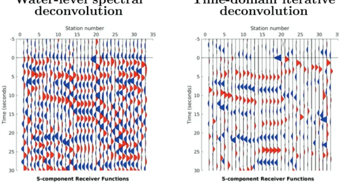
2.3 Deconvolution and receiver functions . . . 142
2.4 Visual inspection of the data . . . 144
3 Methods . . . 145
3.1 2D GRT migration . . . 145
3.2 3D Kirchhoff migration . . . 146
3.3 Multi-mode stacking . . . 148
3.4 Additional data and velocity models . . . 148
4 Results . . . 149
4.1 GRT images . . . 149
4.2 Kirchhoff images . . . 151
5 Discussion . . . 152
5.1 Resolution, penetration and observation limits . . . 152
5.2 Western limit of the Yakutat Terrane . . . 153
5.3 Intra-slab seismicity . . . 154
6 Conclusion . . . 155
Bibliography 161 4 Concluding remarks and scientific outlook 165 1 Conclusions . . . 165
1.1 Writing the migration algorithm . . . 165
1.2 Processing the seismic data . . . 165
1.3 First geological applications . . . 166
1.4 Side projects . . . 166
1.5 Conferences, abstracts and publications . . . 167
2 Scientific outlooks . . . 167
2.1 New geological objectives. . . 167
2.2 Optimizing the numerical algorithm . . . 168
2.3 Adapting the code for new data types . . . 168
Chapter
1
Introduction
1
The Earth: What are we looking at?
1.1
Structure of the Earth
The Earth is round and it orbits the Sun. Although its rough shape and size have been known since at least the ancient Greeks, those findings were later dismissed in the western world before being rediscovered during the past few centuries (Plato, nd). Our planet displays many landscapes that we like to look at, hike through and protect. In its early days, geology started as the field of science that is trying to understand how these landscapes form, evolve and interact. But the Earth also has regions that are subject to various hazards such as earthquakes, volcanoes and tsunamis, and soon geology became a composite science addressing a diverse range of questions such as how the Earth formed and evolved, how these phenomena are generated, and how rocks, oceans and the atmosphere interact among many others.
In geosciences, and in particular in geophysics, direct and indirect observations of processes occurring both at the surface of the Earth and at depth are used to understand its structure and dynamics. A specificity of the geosciences is that they study structures and processes at a wide range of scales both in time and space. If geology started as a very descriptive science, modern geosciences are by essence multidisciplinary, as geoscientists study the Earth with all possible approaches, from field rock sampling to computational geodynamics and isotopic geochemistry.
In this work in particular, we use seismic waves generated by large earthquakes to study the structure of heterogeneities in the first few hundred kilometers inside the Earth (Bostock, 2015). In this first section we will start by diving into the Earth to see what it is made of at the global scale. Then we will explore the surface of the Earth and explain
how we intend to link what we learned from the deeper parts of the Earth to what we see at the surface.
1.1.1 First scientific rationales about the interior of the Earth
Today we know that the Earth is an oblate spheroid and that it describes an ellipsoidal trajectory in space with the Sun as one of the foci, but it has not always been this way (Kepler,1609;Newton,1687). First, until about 3000 years ago in Europe, people thought that the Earth was flat, similar to the ground that we walk on, and probably extended infinitely, as no one ever saw the end of it. Later, during the 6th century BC, the idea of an infinite Earth started bothering the ancient Greeks, and they tried to explain how the oceans and cosmos was wrapped around a finite flat Earth (Aetius, nd). In the 4th century BC, Plato proved that the Earth was round, or more precisely spherical. This made the early geologists wonder what was inside our planet (Aristotle,nd).
Early ideas about the internal composition of the Earth revolve around empty cavities that are linked together and the wind blowing through these cavities was generating the earthquakes and volcanoes. During 2000 years, this hypothesis and other “empty” Earth models, such as the one from Athanasius Kircher, continue to be the predominant view of the interior of the Earth (Kircher, 1664). In the 18th century, Georges-Louis Leclerc, otherwise known as Comte de Buffon, realized that there could not be empty space inside the Earth. The material that this “full” Earth was made of was probably hot, therefore mostly made of molten material, similar to what we would see erupt from time to time in volcanoes (Buffon, 1749). Finally, in the 18th and 19th centuries, geologists started to develop physical methods to test their hypotheses about the composition of the Earth.
1.1.2 Probing the Earth with physical measurements
Physical exploration of the inside of the Earth starts during this period with the formal measurements of the gravity field (figure 1). During his expedition near the Equator to precisely measure the length of a meridian, Bouguer noted that massive mountains should have an observable effect on the gravity field of the Earth given their large mass (Bouguer,1749). However, the effect of the equatorian cordillera on the gravity field was smaller than expected given its size. He did not have a conclusive explanation for that phenomenon, arguing that experiments on other large mountains were required. One century later, two main models were competing to explain these observations.
First, George Biddell Airy said that the gravitational disturbance is mostly compen-sated at depth by a crustal root with similar density (Heiskanen, 1924). Second, John
Figure 1 – Isostasic models. First panel presents the observations described in the text. Second
panel presents the rest state, i.e. without mountain and an unperturbed gravity field. Third and fourth panel present the models developed by Airy (constant density) and Pratt (constant root depth) to explain the geodetic observations.
Henry Pratt said that the disturbance is compensated very shallowly because the moun-tains are made from less dense material than the rest of the Earth (Pratt, 1855). Today, we use the model described by Airy to explain the topography of mountain ranges, and the model described by Pratt to explain the depth of the ocean floor and its topography. Then, scientists went deeper into the Earth using seismology. This new geophysical tool associates the physical principle of the wave equation, formalized by D’Alembert to the study of the Earth’s interior (D’Alembert,1747). By using ground motion recordings at the surface of the Earth, we can record the arrival of compressional (P) and shear (S) waves from naturally occurring earthquakes and artificially generated signals such as quarry blasts, controlled vibrations or even nuclear detonations (Poisson, 1829).
Exploration of the Earth using naturally occurring earthquakes started in 1889 when observation from an earthquake in Tokyo at a station in Potsdam allowed to perform the first estimation of average P-wave velocity in the Earth at around 7km/s (von Rebeur-Paschwitz, 1889). Since then the instrumentation has been, and still is, increasing both in quality and quantity and we have been able to better infer spatial variations in seismic wave velocities inside the Earth. These global observations allowed to probe the Earth deeper and deeper and the first-order seismic structure of the Earth down to its center was established within 50 years of the first quantitative earthquake recording (von Rebeur-Paschwitz, 1889; Lehmann, 1936).
1.1.3 The seismic structure of the Earth
To first order, the Earth is comprised of several concentric layers (Dziewonski and An-derson, 1981). The first layer is the crust, and is separated into continental and oceanic
domains. Then comes the mantle. The limit between these two layers is called the Moho and has been discovered in 1909 by Andrija Mohoroviči`c (Mohorovičić, 1909). It lies at 5 to 10 km depth under the oceans and 30 to 70 km depth under the continents. The mantle is not entirely uniform. There is a region between 410 and 670 km containing three jumps in seismic velocities (Anderson,1967). These fueled the debate as to whether the mantle was acting as one block or as two separate entities. Today we believe that the upper and lower mantle act mainly as one dynamic unit but that these transitions generate some smaller-scale separated dynamics.
At the center of the Earth is the core. The limit between the mantle and the core is called the core-mantle boundary (CMB) and has been proposed by Emil Wiechert in 1897 and formally discovered by Richard Oldham in 1906 (Wiechert, 1897; Oldham, 1906). In 1912, Beno Gutenberg refines the depth of this boundary to its current estimate (Gutenberg,1912). It lies at 2900 km depth, almost uniformly in all regions of the globe. Finally, within the core there is a liquid outer core and a solid inner core. The limit is called the inner core boundary (ICB) and was discovered in 1936 by Inge Lehmann, as the core exhibits an absence of shear wave propagation in the outer part, which is characteristic of a fluid layer (Lehmann,1936). This limit lies at 5200 km depth, and the inner core extends all the way to the center of the Earth at 6370 km depth. The outer core is linked to the Earth’s magnetic field (Gilbert, 1600). Even though the magnetic field has been used for millennia for navigation with compasses, the first theory about its origin dates back only to 1600, and a convincing explanation only emerged in the past century (Gilbert, 1600; Elsasser, 1956). Its origin and behaviour are still debated today, but scientists believe that it is linked to coherent rotation of magnetic fluid, which confirms the seismological observations of a liquid core (Jeffreys, 1926).
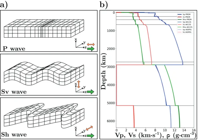
Thanks to the information provided by seismic records, a number of 1D Earth reference models have been proposed (figure 2). One of the first global models obtained from both surface waves and body waves measurements was the preliminary reference Earth model, or PREM (Dziewonski and Anderson,1981). It was computed using normal mode measurements, i.e. the measure of how the Earth vibrates as a whole when excited by very large earthquakes, as well as direct P and S waves travel time measurements. We now have several other 1D Earth models, each one built around different datasets (e.g., IASP91 (Kennett and Engdahl, 1991), AK135 (Kennett et al., 1995)). They represent radial averages of physical properties for any depth inside the Earth. In the case of our seismological models, we can obtain the values of the P and S wave velocities, radial anisotropy, attenuation, as well as the density of the medium. These simple, concentric models serve as a reference for further 2D and 3D imaging methods such as the one
Figure 2 – (a) Geometric representation of P and S waves. Green arrow represents direction
of propagation (always Z) and orange double arrow represents direction of oscillation (Z for P wave, X for Sv wave, Y for Sh wave). (b) Reference 1D Earth models elastic parameters.
developed during this thesis (see section3 and chapter 2).
In order to decipher the thermo-chemical structure of the Earth, seismic velocities computed for the Earth are compared with laboratory experiments to find which mate-rials and temperatures are the most probable candidates. At first, pure elements and minerals were tested for density and seismic velocities under broad ranges of pressure and temperature conditions. This is how we found that the core is mainly made of iron and the mantle made of silicates (Anderson et al., 1971; Badro et al., 2007). To further dis-criminate between the candidate rocks, which represent different chemical compositions for the Earth, we need to be able to replicate the jumps in elastic properties from the seismological models. This is how we constrained the silicate composition of the mantle (Duffy and Anderson, 1989; Xu et al., 2008). Finally, we can add constraints from other fields such as gravimetry and cosmochemistry to refine our estimates. This field is still very active today as the sensitivity from the different methods increases and the estimates become more precise.
mod-els, scientists wanted to go further and understand the structure and evolution of a 3D dynamic Earth. Therefore, the next step is to describe the Earth using 3D models. In such models, the specific aspects of different regions of the Earth can be explored inde-pendently, or studied together to investigate the structure and evolution of our planet at the global scale. These 3D studies and models can be done on a global scale or a regional scale and target a large variety of different phenomena. This thesis deals mainly with structures in the upper few hundred kilometers of the Earth, at the interface between the mantle and the crust. We are interested in how the mantle and the crust interact with each other when two tectonic plates collide. The lateral extent of the regions that we are interested in is on the order of a few hundred kilometers, placing it at the intermediate “continental” scale.
1.2
The surface of the Earth: the tectonic plates and their
boundaries
1.2.1 From the fixist Earth to plate tectonics
Going back briefly to the surface of the Earth, we will now look at how it moves, and more particularly at how tectonic plates interact with each other. The idea of a laterally evolving Earth surface made of moving elements, where the current proportions and distribution of ∼70% oceans split into 3 main bodies of water and ∼30% land split into seven main continents changes through geological ages, is quite recent in scientific history (Suess, 1885). First, people believed in the hypothesis of the fixist Earth, which states that the Earth has always existed in its current form. This fixist point of view is a broader mode of thinking than just geology, and also applied to the nature of animal species for example, as the dominant hypothesis for thousands of years.
When the Earth was proven to be round for the second time in western history (see section1.1), the idea of the collapsing Earth took its place (Suess,1885). This theory links the thermal state of the Earth, which at that time is believed to be made of extremely hot and dilated material, to that of a cooling solid body. By virtue of cooling the Earth, therefore reducing its volume while keeping the same surface area, the cooling Earth theory explains the creation of the mountains by way of preferential collapsing in some parts of the globe. This theory also aimed at explaining other geophysical phenomena, such as earthquakes, but failed at capturing the nature of their distribution on the globe (Bonnier, 1900).
these views (Wegener, 1929). Wegener uses geometrical and paleontological clues, most famously the intricate puzzle pieces that some continental shelves form, common glacial clues on several southern continents as well as shared fossil record across oceans, to prove that the continents must have been in a different configuration in the past. However, his theory was not complete as he lacked a proper driving force to explain those mouvements.
In the 1950’s and 60’s, Harry Hess and others found new observations and a driving force that confirm the lateral motion of the ocean floor (Hess, 1962). After the discovery of the high topography and seismic activity of the central part of the seafloor, the mid-oceanic ridge, they observed magnetic bands on the ocean floor. Those magnetic bands are symmetric in polarity and age on either side of the ridge, with younger ages closer to the ridge, which indicates the ocean floor is moving away from the ridge. Hess explains that this lateral motion is supported by global convection in the Earth’s mantle. Based on these observations, Jason Morgan, Xavier Le Pichon, and Dan McKenzie independently proposed quantitative surface motion models that separate the Earth in 6 to 12 major plates between 1967 and 1968 (McKenzie and Parker, 1967; Morgan, 1968; Le Pichon, 1968). This was the birth of the plate tectonics theory.
The structural definition of a plate has emerged in the 1960’s with the birth of the plate tectonic theory and precise seismological observations (McKenzie and Parker,1967). This theory states that there are a few rigid bodies that travel across the surface of the Earth and that are in contact with one another at moving boundaries where matter is extracted from or injected into the mantle. These boundaries accumulate and relieve most of the stresses due to the tectonic activity of the Earth, and are strongly underlined by the distribution of earthquake hypocenters, as can be seen on figure3.
Seismological observations show that the plates themselves are dynamically decoupled at depth from the unperturbed upper mantle by a low velocity zone (LVZ) that usually lies at up to a few tens of kilometers depth under the oceans and up to a few hundred kilometers depth under the continents (Chapman and Pollack, 1977). The tectonic plate is seismologically defined as everything that is above this discontinuity, event if this seis-mological signal is not clear in every region of the Earth. It is comprised of a piece of crust, continental or oceanic, and lithospheric mantle. The tectonic plates, especially the continental ones, usually have a complex and rich history. Some pieces of continental crust have been dated at up to 4 billion years, which is barely 500 millions years after the formation of the Earth (Bowring et al., 1989).
Figure 3 – Map of tectonic plates today. Triangles represent convergent limits, dashes
repre-sent divergent limits. W-A=west Africa, E-A=east Africa, N-A=North America, S-A=South America, An=Antarctica, Ar=Arabia, Au=Australia, Ca=Carribean, Co=Cocos, Eu=Eurasia, In=India, Na=Nazca, Pa=Pacific, Ph=Philipine. Image reproduced from tectonicwaters. wordpress.comusing data from Peter Bird (Sornette and Pisarenko,2003).
1.2.2 Interactions at the plate boundaries
The different tectonic plates interact with each other at their common boundaries. These boundaries can be divergent, i.e. the plates move away from another, convergent, i.e. the plates move closer to another, or strike-slip, i.e. the plates glide by another. These structures highlight the limits between different regions of the Earth’s surface, that have different structural properties, and present some of the largest natural risks. The most prominent and direct risk is earthquakes. They happen when stress, that is slowly accu-mulated for long periods of time due to friction between plates that move relative to each other, is suddenly released between them and they slip along their interface (Savage and Prescott,1978). This releases seismic energy that can damage buildings in the near field and propagate strong waves in the far field. We will talk about them in abundance later. Another risk associated with plate boundaries is the generation of tsunamis. Tsunamis are large oceanic waves that are not generated by tidal motion, usually of very long wavelength, that propagate across the oceans and hit the land where they can reach high amplitudes due to the shallow sea level (Satake, 2015). They can happen after strong offshore megathurst earthquakes that shake the ocean floor vertically, thus generating large waves above their hypocenter.
Finally, plate boundaries are associated with volcanoes. The best example is the ring of fire in the Pacific ocean, but one can also cite the Krakatoa volcano in Indonesia, mount Vesuvio or Etna Italy and Tristan da Cunha or the Canary islands in the middle of the Atlantic ocean (Marsh,2015).
Plate boundaries mainly take the shape of line segments when viewed from the top. Some of those segments have a certain continuity along strike, such as the plate boundaries around the Pacific ocean. As it is difficult to represent complex structures in 3D, we usually study their structure by looking at transects oriented orthogonally to their strike (Rondenay, 2009). These 2D transects reveal a limited number typical 2D structures that can be observed across many different regions. We will describe them in the next paragraph. When continuity is less obvious in map view, such as in the Himalayan mountain ranges for example, this usually translates into more complex 3D structures underneath (Priestley et al., 2008).
There are three main types of 2D structures at plate boundaries (figure 4). They represent steady-state behaviours of plate boundaries. The first ones are the mid-oceanic ridges that we described earlier (Dunn,2015). Those are regions, hidden under the oceans, where extension between two plates makes mantle material rise and partially melt to create new oceanic crust. The second ones are transform faults (Wessel and Müller,2015). Those are regions where two plates are in contact with each other but no crustal material is created from nor injected into the mantle. Most of them are also on the ocean floor, and connect segments of the spreading ridge. The third ones are subduction zones (Wada and King, 2015). Those are regions where a slightly denser plate, usually of oceanic nature, is forced to enter the Earth under a slightly more buoyant plate, usually of continental nature. Hence in this case crustal material is injected into the mantle. We will describe this in greater detail later. These structures are mostly 2D and have symmetries along the direction of mouvement between the plates.
In addition to these mainly 2D structures, there a few fully 3D structures (figure 4). They correspond to very particular environments and/or initiation and termination of the processes cited above. The two most prominent examples are rifting zones, where mid-oceanic ridges are born, and suture zones, where subduction terminates (Searle, 2015; Buck, 2015). A third type of 3D structure occurs in regions where the tectonic setting goes from one type of boundary to another. For example when a plate boundary goes from a subduction dynamic to a stage of suture/collision, or from frontal subduction to strike-slip motion (Pearce et al.,2012). This is what we will study in chapter 2. Finally, introducing a large scale heterogeneity in what is mostly a 2D setting, such as a subduction zone, can generate strong 3D behaviour. This is what we will study in chapter3.
Figure 4 – Simplified 2D view through typical plate boundary structures, not to scale.
Trans-form faults are not shown here as they are mostly parallel to this kind of slice, visible only in map vue.
1.3
Subduction zones
A subduction zone is a complex open system. It is linked to the recycling of crustal material in the upper and lower parts of the mantle and to the cycle of a large number of elements and molecules, including CO2 and water (Dasgupta and Hirschmann, 2010). Subduction happens when a plate is pushed under another one into the mantle, potentially all the way down to the core mantle boundary. Its dynamics are linked to differences in mineralogy and temperature between the plates, which in turn create large density variations (Jamtveit et al., 1990). These density variations determine which plate sinks and which stays afloat.
In the most general sense, subduction can happen between any two plates but almost always implies at least one oceanic plate. The chemical composition of oceanic plates is slightly different from continental plates (Mooney,2015). Oceanic plates contain less silica overall, which makes them denser and less rigid. This means that when a continental and an oceanic plate collide, the continental one has a higher buoyancy and tends to override the oceanic one rather than deform to accommodate the stress. This pushes the oceanic plate into the mantle, increasing the lithostatic pressure that it is subject to (figure 5).
Oceanic plates are normally more buoyant than the mantle, which should prevent them to sink even if they are trapped under a continent (Wada and King, 2015). However, the increase in pressure, as well as temperature to a smaller extent, triggers a series of mineralogic reactions in the oceanic crust (Doin and Henry, 2001). These reactions, culminating with eclogitization, increase the density of the oceanic plate to above that of the mantle, therefore making the oceanic plate sink into the mantle.
The fate of the plate that subducts is further mineralogic transformation, bending, and exchange of material with the surrounding mantle (Fukao and Obayashi, 2015). During the subduction process, the minerals react with each other to create new ones in the solid
Figure 5 – Simplified 2D view of a subduction zone. Metamorphic facies are given for the
oceanic crust (gray). Yellow is oceanic lithospheric mantle. Blue arrows represent main dehy-dration locations along progressive phase transformations in the subducting crust
state. This is called metamorphism, and specific mineralogic compositions corresponding to specific pressure and temperature conditions are called facies. The first facies that a subducting oceanic crust goes through are the unperturbed basalts and gabbros. Those rocks then go through the greenschist facies, followed by the blueschist facies, amphibolite facies and finally the eclogite facies. This last reaction is what we defined as eclogitization earlier.
Every transition is characterized by a change in density as well as in volatile elements content (Kerrick and Connolly,2001). Eclogitization in particular releases large amounts of water from the crustal minerals. The mouvement of water in and out of the oceanic crust and potentially mantle is helped by the bending, and subsequent unbending, of the sinking plate entering the subduction zone (Buffett and Becker, 2012). These rotational motions create preferential pathways for the fluids to migrate, as bending at the surface as the plate start to dip towards the mantle creates faults where the water can infiltrate the crust and hydrate crustal minerals, therefore entering the subduction system. When the plate reaches a stable dip at about 20 to 50 km depth, it bends in the other direction to become flat again, which we call unbending (Singh et al.,2012). This creates new fractures that favour fluid exchanges in the system. Upon escaping the crust at the eclogitization state, the water hydrates the surrounding mantle, and thus facilitates the formation of
magma (Van Keken et al.,2002). This results in volcanic activity in the overriding crust. This activity depends on the hydration and thermal state of the subducting plate and therefore vary largely from region to region.
The subduction system is even more complex as it interacts with sedimentology rates and climate (Lamb and Davis, 2003). The first mostly has an effect on the hydration of the crust and the frictional behaviour of the interface, while the latter is influenced by the surface expression of the subduction in the form of the cordilleras, volcanic arcs and medium-to-large-scale intra-plate basins that can form in the back-arc. In turn, a strongly erosive climate such as the monsoon system can increase the sedimentation rate in the oceans, therefore affecting the friction of the subduction interface.
Previously, we classified subduction as a mostly 2D phenomenon, although there are always along-trench variations. The 2D properties of the subduction system, which are overall similar for subduction zones around the globe, help us get a good first order idea of the dynamics of the system. However, the fine 3D structure of every subduction zone is different. In our study, we will look at 2 regions in particular and analyze their 3D structure. The first one is western Greece. It is the place where the oldest oceanic lithosphere is still subducting today (Speranza et al., 2012). It sees the subduction of 230 million years old oceanic plate in the Mediterranean under the european continental plate. Being very close to termination on a geological time scale, it presents strong 3D patterns such as a pronounced bend from the north west in the Balkans to the south east and then east in Turkey. This makes 2D imaging challenging.
The second one is southern Alaska. It is at the intersection between the Aleutian subduction, where regular oceanic plate subducts mostly perpendicularly to the trench, and the North American cordillera, which subducts in the opposite direction as it crosses the Pacific ridge (Martin-Short et al., 2018). This setting is complex and the variation in the properties of the subducting material, as well as the orientation of the subduction, make it a strongly 3D setting. We will look at those two subduction zones using teleseismic imaging, which we will explain in the next sections.
2
Which tools do we have to image the Earth?
2.1
Geophysical exploration
One of the first geophysical tools used to explore the Earth was gravimetry (Jekeli,2015). As described previously, it was used to discover the crustal roots of mountain ranges (Bouguer, 1749). Nowadays, the gravity field and its anomalies can be measured very
accurately from space using satellites (Tapley et al., 2004). Gravimetric studies are still actively used today, to study the composition of crustal anomalies in mountain ranges, or the characteristics of large earthquakes that happen in subduction zones for example (Panet et al., 2007).
Another type of geophysical exploration is electromagnetic sensing. It probes the electric conductivity and magnetic potential in the Earth (Fitterman, 2015). Changes in the magnetic field can be linked to variations in the dynamic of the core, which in turn affect aspects like the secular cooling of the Earth or volatiles transport from the inner core to the CMB (Cardin and Olson, 2015). Changes in the dynamics of the Earth’s core have also been hypothesised to be linked to the formation of hot mantle material, called plumes, that rise from the CMB to the surface and can lead to continental size volcanic eruptions and continental breakup, both of which have been associated with mass extinctions (Ballmer et al., 2015). Changes in the electrical conductivity inside the Earth can be used to track the presence of various conductive elements and minerals. It is for example very sensitive to the presence of fluids such as free water in rocks (Worzewski et al., 2011). This makes it an effective tool to look at the dehydration in subduction zones that we described earlier.
The geophysical tool that we are probing the Earth with in this work is seismological analysis (Dziewonski and Romanowicz, 2015). As described in section 1.1, it uses the properties of the waves that travel through the Earth after it has been excited by a seismic event. This allows us to characterize the Earth in terms of velocities of wave propagation and density. These parameters can then be turned into information about the lithologies and thermodynamic conditions by combining the seismic observations with results from laboratory experiments. The triggering event can be natural (in this case the field of study is called passive seismology) or man made (in this case the field of study is called active seismics).
2.2
Seismic imaging
As stated above, there are two main ways of probing the Earth with seismic waves (6). We will first focus on active seismics, which uses man made seismic waves. In this case, one artificially creates seismic waves at the surface of the Earth using explosive or vibrating sources, and records them on dense arrays of receivers (Levander et al., 2007). This can be done on land or offshore. There are copious amounts of techniques that are used to exploit these data.
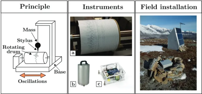
Figure 6 – Seismic instrumentation. Principle of analog seismograph recording. The stylus
and mass do not move with respect to the unperturbed Earth referential. The base and rotating drum are subject to the oscillations caused by the seismic waves, hence the information can be quantitatively recorded. Image from instrument (a) is taken from wikipedia.org, instrument (b) from guralp.com, instrument (c) from raspberryshake.org and field installation from
earthscope.org.
generate a well defined and known signal because we know the location and form of the source. This allows for easy data processing of the waveforms and clear identification of primary (incident P and S waves, see section 2.3) and secondary phases (scattered wavefield, see section 2.4) even without heavy treatment of the data. Second, the data can be recorded only when needed. There is only minimal data storage space wasted, and less processing to do after the recording of the waveforms. Third, the recording units, or seismic stations, can be chosen accordingly to the characteristics of the source. This means that the sensitivity, orientation and sampling rates of the instruments can be tuned to best suit the expected response based on their location relative to the source. Fourth, as a consequence of all previous advantages, the data coverage can be optimized for any study area or target. As an example, one can choose to use larger instruments on a larger area if the study sites are easily reachable, or smaller instruments in close vicinity if the locations are more difficult to access.
The drawbacks of active seismic experiments are that deploying many receivers can be time consuming and that most source generation methods are expensive to operate and maintain. Also, the waves generated with conventional techniques do not travel very far in most cases. This is because the energy they release is limited and their typical frequency range is above 1Hz, hence the waves are subject to high attenuation values.
This limits the volume that can be probed using a single study configuration.
The second way of determining seismic velocities and contrasts inside the Earth is passive seismology (Steim,2015). In this case one uses the energy radiated from natural earthquakes occurring only hundreds of meters or up to thousands of kilometers away from the target area. This has several advantages over active seismics. First, naturally occurring earthquakes can illuminate the Earth from the interior, not only the surface. Intermediate depth and deep earthquakes provide not only information about the pro-cesses at play in their origin region, but also valuable information about the medium they propagate through on their way to local seismic receivers (Halpaap et al., 2019). Second, large earthquakes radiate seismic energy that travels across the entire Earth and can be recorded thousands of kilometers away. Because the forces at play in plate tectonics are several orders of magnitude higher than those of active seismics, sometimes dwarfing the largest nuclear detonations, the waves these earthquakes generate travel through all the layers in the Earth and provide unique information about the deep structure of our planet. The main drawbacks of passive seismology are linked to the fact that these type of earthquakes cannot be controlled (Madariaga, 2015). First, they happen at random times, which means that we need to constantly monitor them to be able to record the information. Even though we can statistically estimate how many earthquakes of a given magnitude should happen in any given time period, we do not have the ability to predict individual earthquakes, be it in terms of timing or magnitude. Second, they are linked to tectonic processes and therefore only happen in specific regions around the world. This means that the data coverage cannot be perfectly optimized for specific studies. This can however be partly mitigated after large earthquakes that are followed closely by smaller earthquakes that release residual stresses, called aftershock sequences (Helmstetter and Sornette,2003). Finally, unlike the artificial sources, they have complicated uncontrolled source signatures, or source time functions (STF). This can make it very hard to extract the desired signal needed for imaging within the complete recorded signal (Houston,2001). In addition to that, the amount of radiated energy is not azimuthally uniform. This is because natural earthquakes happen when tectonic faults abruptly move relative to another, and so the sources are characterized by two opposite motion vectors separated by a plane (Zhu and Helmberger,1996). On either side of that plane, part of the material is compressed (the part that is at the tip of the vector), while the other part of the material is dilated. This creates four distinct regions, called quadrants, across which the source function varies. Finding the best way to extract the information from complicated waveforms is an active field of research that we will explore in section 4 of this chapter and in chapter3.
Because they aim at exploring different parts of the globe and at different scales, active and passive seismic studies also face different challenges in terms of how they use the data to produce images of the Earth. In order to understand exactly how the methods developed for both fields differ, we need to describe the seismic wavefield in greater detail, starting with the difference between the direct, scattered, reflected and diffracted wavefields.
2.3
The incident wavefield
The wavefield can be separated into incident and scattered wavefields. The scattered wave-field can be further separated in reflected and diffracted wavewave-fields. The incident wavewave-field corresponds to the solution of the wave equation in a layered, internally smooth, Earth model (Bostock, 2015). For teleseismic waves, it is composed of the primary compression body wave, called the P wave, the secondary shear body wave, called the S wave, the body waves that reflect at, or interact with, the major boundaries inside the Earth such as the CMB (e.g., PKP, SKS, SCS) or ICB (e.g., PKIKP) and the surface waves (see figure7).
In the following, we will mainly be interested in the incident P and S body waves. As shown in figure 2, they oscillate in different directions, and have different velocities, with S waves being typically slower than P waves. They travel through the Earth following Huygens’ principle (Huygens, 1690). Their velocities depend on the elastic parameters of the Earth, namely the Lamé parameters λ and μ and the density ρ (Lamé, 1852). Those, in turn, are linked to the nature of the materials inside the Earth, and using our seismological tools we hope to resolve the composition and temperature of the Earth by mapping these parameters at depth.
One of the most used tools to estimate the elastic parameters of the Earth using the incident wavefield is called tomography. Similar to medical tomography, it uses the propagation path of the seismic waves inside the Earth and their travel times to estimate these parameters (Thurber and Ritsema, 2015). Knowing how long it takes for a wave to travel from the source to the receiver allows us to get access to its mean propagation velocity along its path. In order to compute the travel path of those incident waves, one usually has to resort to the infinite frequency approximation to provide the most direct path from a source to a receiver in a given Earth model (Buland and Chapman, 1983). Using inversion techniques and several sources and receivers, one can recover local wave velocities from these average results. This is the field of seismic travel-time tomography. A short example of how it works for a 2D case is shown in figure 8. In this case, there are 2 sources and 2 receivers, hence 4 rays going through the imaging region. The
Figure 7 – Main phases from the incident wavefield on a slice of the Earth. Star represent the
hypocenter of the source earthquake. K is the name of a P wave inside the outer core, I inside the inner core, and C is a reflection at the CMB.
region has been separated in 9 areas to invert for seismic velocities. Squares A2 and B1 have one ray passing through, A1, A3, B2, C1 and C2 have two rays going through, and squares B3 and C3 have no rays traversing them. Also, there are only 4 rays for 9 velocities, which means that the system is ill-posed. Using this data and a simple linear tomography method, one could to obtain velocity values for the first 7 squares, albeit with large trade-offs, while values for the two orange squares are completely unconstrained.
Travel-time tomography is powerful but is limited by the data coverage and inversion parametrization, and rely on implicit or explicit regularization factors in order to provide an interpretable image of the Earth (Kissling et al., 2001). There are various ways to regularize the tomographic problem, but most methods rely on two main approaches (Charlety et al., 2013). The first main type of regularization is damping, where one tries to stay as close as possible to a pre-established vision of the Earth while still being able to explain the observations. In the case of the previous example, choosing a pre-established value for the velocity in each square before the inversion would constrain the inverted
Figure 8 – Simplistic arrival time tomography. Here 7 out of 9 squares have rays passing
through them, sampling information along the way, and there is no ray, i.e. no information, going through squares B3 and C3.
velocity values for squares B3 and C3.
The second main type of regularization is smoothing, where values from a given pa-rameter cell would affect the neighbouring cells to a certain extent while still explaining the observed arrival times. This usually allows to smooth out the small-scale variations that can arise when using noisy data. In the case of the previous example, a smoothed inversion would use the values from squares A3, B2 and C2 to constrain the inverted value and obtain a model with 9 velocity values. More advanced, iterative tomographic methods use adaptive parameterization in order to alleviate some of those drawbacks, or include data from the scattered wavefield to add more constraints on the inverted velocity models (Bodin et al., 2009).
2.4
The scattered wavefield
The scattered wavefield corresponds to the late arrivals recorded after the incident wave-field (Bostock,2015). It represents the residual solution of the wave equation in a realistic, sharp Earth model after the incident wavefield has been removed. The scattered wavefield is comprised of all the reflections and diffractions that the incident wavefield generated when it interacts with the scattering structure of the Earth (figure9). The scattered waves typically have a smaller amplitude than the incident wavefield and they can adopt a very complex shape with increasing number of interactions. By nature, they are linked to the
Figure 9 – (a) Scattering geometry for a point scatterer. (b) Elastic scattering patterns
rep-resent the amplitude and polarity of the outgoing scattered wave depending on its orientation to the incoming wave. For example, P-to-S scattering with δβ/β has very low, negative for-ward scattering amplitude following the direction of the incoming wave, but strong scattering amplitude at 45° forward (negative) and backward (positive).
scattering heterogeneities, and therefore hold information about the fine scale structure of the Earth. The scattered wavefield has been used extensively in the field of active seismics and is becoming a prominent tool to study the Earth through passive seismology (Rondenay,2009).
2.4.1 Active seismic experiments
The scattered seismic wavefield has be used in many ways over the past decades. One of its best known uses in active seismics is seismic reflection (Knapp and Steeples, 1986). In this method, one records the wavefield generated by artificial sources long after the incident wavefield to record the impulses of energy that travel down the Earth and are reflected at discontinuities inside the Earth (figure 10). It is used to characterize the location of interfaces inside the Earth. Reflection seismics follow the same basic ideas as travel time tomography, but this time instead of assuming a propagation path and looking for a velocity model, one assumes that the velocity of the wave through the medium is known and use the arrival times of the different scattered phases to infer the depth at which they were converted or reflected, i.e. their path. The velocity model can take the form a homogeneous velocity, a layered model or even a 3D model.
As in travel time tomography, the level of resolution can be enhanced by having multiple source-receiver configurations that illuminate the same depth points (Tarantola,
1984). However, opposite to travel time tomography, the improvement does not rely on the inversion, but rather on clever stacking of the signals to enhance the signal to noise ratio
(SNR) and obtain the image that shows the structures more clearly (Mayne,1962). This means that there is no explicit regularization in this case, but that the velocity model that one assumes for the wave propagation becomes a critical factor for the imaging condition. One method in particular, called Kirchhoff migration, will be of interest to us. It follows developments that started in the 1920’s and was fully theoretized by 1954, as part of an array of methods aimed at 3D imaging of subsurface reflections (Hagedoorn, 1954). The basic principle can be explained as follows, and will be expanded upon later. In this imaging principle, the recorded wavefield is propagated back into the Earth from the receivers to the sources, i.e. backwards in time, at all potential scattering points. The migration method identifies the location of scattering points using the interference between the different waveforms, i.e. through constructive stacking.
The other main technique using the scattered seismic wavefield in active exploration is large offset seismic refraction (Lankston, 1990). In that case, one seeks to record not only the waves that reflect off interfaces but also the leading waves that travel exactly along these interfaces (figure 10). The properties of these waves allow the operator to retrieve seismic velocities in addition to the position of the interfaces (Yilmaz, 2001). Indeed, not only do these waves travel at the interface between two media, which is what we want to image, but they also travel at a velocity that corresponds to the fastest of the two media. By aligning the recordings and sorting them by distance, one can estimate the velocity in any given layer by looking for the value that gives the most coherent result for a given head wave (Zelt et al.,2003). This can then be repeated for every head wave at increasing depths, which will produce an updated velocity profile that is closer to the reality than the original one. These methods, which have been combined with reflection approaches in a coherent imaging theory over the past few decades, are very useful for oil and gas field discovery, but also seismic characterization of deep crustal structures (Rawlinson et al., 2001; Brocher et al., 1994).
2.4.2 Passive seismology
In passive seismology, there are many different scattered phases that can be used. They provide information about the scattering structure of different regions in the Earth. Fig-ure11shows the three main regions around the path of the seismic waves where scattering takes place. During the rest of this chapter, we will only consider seismic phases that are scattered a single time. This is referred to as the Born approximation, and has proven to be effective at explaining most of the observed waveforms (Miles, 1960; Hudson and Heritage, 1981).
Figure 10 – Geometry of offshore active seismics acquisition. Reflected energy gives direct
information about the depth of the reflectors and the impedance contrast, whereas refracted head waves give information about the velocity of the medium.
The first region where scattering is an important factor is on the source-side. The most pronounced seismic phases coming from this region are the pP and sS phases, commonly referred to as depth phases (Wang and Zhao,2005). They travel from the source directly to the surface (lowercase phase identification letter) and from there to the receiver (uppercase phase identification letter). In seismically active regions where there are strong, relatively flat layers with strong low velocity contrasts, the waves can be subject to critical reflections inside these layers. For example, in subduction zones, the low velocity layer in the top part of the subducted crust can act as a waveguide (Abers, 2005). These phases are usually considered as part of the non-random noise recorded at seismic stations, but can be used to our advantage and give us information about the precise location of the sources (Halpaap et al., 2019). For teleseismic receiver-side studies, these signals however only act as one more complexity in the source function.
Later along the path of steep waves, scattering can happen in the lower parts of the mantle. This is mainly observed on the incident PKP and SKS waves, which are phases that cross the CMB and travel through a part of the Earth’s core (Vidale and Hedlin,
1998; Thomas et al., 1999). This type of scattering can generate PKP precursors for instance, which are linked to low velocity anomalies and partial melting at the CMB on either side of the travel path. These anomalies make certain branches, or ray paths, of the phase faster than the dominant PKP branch (called PKPdf) and this delay gives us