HAL Id: hal-01296738
https://hal.archives-ouvertes.fr/hal-01296738
Submitted on 1 Apr 2016HAL is a multi-disciplinary open access archive for the deposit and dissemination of sci-entific research documents, whether they are pub-lished or not. The documents may come from teaching and research institutions in France or abroad, or from public or private research centers.
L’archive ouverte pluridisciplinaire HAL, est destinée au dépôt et à la diffusion de documents scientifiques de niveau recherche, publiés ou non, émanant des établissements d’enseignement et de recherche français ou étrangers, des laboratoires publics ou privés.
Real wage cyclicality in the Eurozone before and during
the Great Recession: Evidence from micro data
Gregory Verdugo
To cite this version:
Gregory Verdugo. Real wage cyclicality in the Eurozone before and during the Great Recession: Evidence from micro data. European Economic Review, Elsevier, 2016, �10.1016/j.euroecorev.2015.11.001�. �hal-01296738�
1
Real Wage Cyclicality in the Eurozone before and
during the Great Recession: Evidence from Micro Data
Gregory Verdugo
Centre d’Économie de la Sorbonne, Université Paris 1
Abstract
We study the response of real wages to the business cycle in eight major Eurozone countries before and during the Great Recession. Average real wages are found to be acyclical, but this reflects, in large part, the effect of changes in the composition of the labour force related to unemployment variations over the cycle. Using longitudinal micro data from the ECHP and SILC panels to control for
composition effects, we estimate the elasticities of real wage growth to unemployment increases between −0.6 and −1 over the period 1994-2011. Composition effects have been particularly large since 2008, and they explain most of the stagnation or increase in the average wage observed in some countries from 2008 to 2011. In contrast, at a constant labour force composition in terms of education and experience, the figures indicate a significant decrease in average wages during the downturn, particularly in countries most affected by the crisis. Overall, there is no evidence of downward nominal wage rigidity during the Great recession in most countries in our sample.
JEL Codes: J30, E32
Keywords: Wage cyclicality, wage rigidity, Great recession, Euro zone
Email: gregory.verdugo@univ-paris1.fr . Address: 106-112 Boulevard de l'Hôpital, 75647 Paris cedex 13, France. Much of this research was done while the author was at the Banque de France. The author is grateful to Laurent Baudry from the Banque de France for his excellent research assistance. The author also thanks the associate editor, two anonymous referees, Mario Izquierdo, Felix Koenig and Pedro Portugal for insightful comments on a previous draft which have substantially improved the paper. Many thanks also to seminar participants at the 4th SOLE-EALE World Conference in Montréal, the IZA Workshop on Wage Rigidities and the Business Cycle in Bonn, the
IZA/NBS/CELSI Conference on European Labour Markets and the Euro Area during the Great Recession in Bratislava and the Conference on Firm’s Behaviour in the Crisis of the Banque de France in Paris for insights that helped to shape the paper.
2
Introduction
In the first years of the Great Recession in the Eurozone, aggregate real wages did not react
significantly to the downturn, particularly in countries most affected by the crisis. These developments raised serious concerns about the long-term viability of the Eurozone. Wage flexibility is viewed as crucial in a currency union where internal migrations until now have been too low to ensure a significant macroeconomic adjustment (Anderton et al., 2012; Krugman, 2013). A combination of fixed exchange rates, low inflation and downward nominal wage rigidity creates real rigidities (Schmitt-Grohé and Uribe, 2013). As the labour market does not clear, involuntary unemployment increases following patterns originally described by Keynes (1925) or Friedman (1953). According to this narrative, downward nominal wage rigidity might thus be partly responsible of the current unemployment crisis in the periphery of the Eurozone.
However, most of the evidence that wages were relatively rigid during the Great Recession relies on aggregate data from national accounts. These figures are the only comparable cross-country data that are rapidly available, but they are not without limitations. An important shortcoming is the difficulty in interpreting their evolution, particularly during exceptional crisis periods, if the
composition of the labour force changes significantly over the cycle.
Cyclical changes in the composition of the labour force reflect the fact that, empirically, unemployment disproportionately concerns low-wage workers.1 When unemployment increases, the labour force becomes older and more skilled. This affects the average wage in a counter-cyclical way; the average increases mechanically because the share of low-wage workers in the population
1
See Chirinko (1980), who shows that low-wage workers are more affected by unemployment than high-wage workers during recessions.
3 diminishes. When these composition effects are large, they may mask the response of wages to the cycle in the aggregate series.
Many studies have shown that compositional biases are quantitatively important in aggregate data since Bils (1985) and Solon, Barsky and Parker (1994). This issue is also discussed in standard macroeconomic textbooks (Romer, 2006 p. 264) as understanding whether wages are rigid is quite important to discriminate between theoretical models of macroeconomic fluctuations (Swanson, 2004). 2
Surprisingly, composition effects during the Great Recession in continental Europe have received relatively little attention despite the fact that unemployment changes have been particularly dramatic.3 From 2007 to 2012, unemployment increased by 16 p.p. in Spain, 7.8 p.p. in Portugal, and 4.6 p.p. in Italy. Unemployment has affected unskilled and young workers in a particularly severe way, and as a result, the characteristics of employees changed dramatically. In Spain, the share of less educated workers among employees decreased by 8 p.p. from 44% to 36% between 2007 and 2012, while the share of university graduate workers increased symmetrically by 8 p.p.4 Because of these large changes, it is unclear how much the evolution of aggregate wages during the Great Recession in these countries reflects a change in the price of labour or in the composition of the labour force.
More generally, whether wages are relatively more rigid in Europe than in other countries remains an open question. While some important and recent works using micro data to estimate the
2 While modern approaches are less clear-cut, the real business cycle models initially proposed by Kydland and
Prescott (1982) posit that economic fluctuations reflect exogenous shocks to the economy’s technology. These models are consistent with a procyclical relationship between real wages and employment, as wages adjust to shocks. In contrast, for classical or traditional Keynesian models, wage stickiness explains the cyclical volatility of employment.
3 A recent exception is provided by Blundell, Crawford and Jin (2014) on the UK. Because unemployment in the
UK did not increase as much as in continental Europe, they find little difference between aggregate wage series and series adjusting for composition effects.
4 cyclicality of wages are now available for several major European countries5, comparisons are
difficult, as the construction of the sample, data source and period vary in potentially significant ways across studies. Most of these studies were also conducted before the recent crisis, and the importance of wage rigidity in the recent period remains an open question.
In this paper, we use harmonised panel micro data from the period 1994-2011, covering eight major countries of the Eurozone, to examine the relationship between real wages and the business cycle before and after the Great Recession. As in previous work, we find that aggregate real wage series are not cyclical. However, when we account for changes in the composition of workers using individual data, we find that this acyclicality reflects the consequences of compositional changes in the labour force. We obtain statistically significant elasticities of real wage growth to unemployment changes of between −0.6 and −1.6 These values are quite close to those reported in the existing literature for the US but are nevertheless lower than those for the UK in recent studies.
However, panel data is not always available, and even when they are, they might not be rapidly released which prevent the analysis of recent periods. To test the importance of relying on panel data, we assess whether using cross-sectional data, which is more easily available, affects the estimates in our sample. Instead of using individual fixed effects to account for composition effects, we use flexible controls for education and potential experience through the interaction between eight cells of potential experience and three levels of education. While far from perfect, we find that such method is able to account for a large share of the composition biases. The estimated coefficient is found to be negative and is measured relatively precisely, but it is slightly smaller, close to −0.42.
5
See Anger (2011) for Germany, Peng and Siebert (2008) for Italy, Verdugo (2013) for France and Carneiro, Guimarães and Portugal (2012) for Portugal. For non-European countries, see also Shin (2012) for Korea, Devereux (2000) for the US and Devereux and Hart (2006) for the UK.
6 In practice, as we regress changes in log wages on changes in the unemployment rate in percentage point (and
not in log), we estimate “semi-elasticities”. We use the term “elasticity” in preference to the “semi-elasticity” for simplicity and brevity.
5 During the Great Recession, we find that the apparent rigidity of average real wages in the aggregate data has been substantially exaggerated by composition biases. Most of the increase or stagnation in real wages in aggregate series can be explained by composition effects, particularly in countries most affected by the downturn. When we control for composition, we observe that real wages responded significantly to the downturn.
Some evidence suggests that the adjustment is heterogeneous over the distribution of wages. We find a much higher elasticity of wage growth for workers in the first decile than in the rest of the distribution. Consistent with the existing literature, the elasticity of job changers is found to be double that of job stayers. On the other hand, there is little evidence that wages adjust additionally to region-specific unemployment shocks. This implies that within countries, most of the adjustments to a negative regional labour demand shock will depend on internal labour mobility.
In the second part of the paper, we examine in detail the distribution of individual wage changes in order to study the interplay between inflation and wage adjustments. A particularly interesting aspect of our dataset is that half of the countries in the sample (France, Finland, the Netherlands and Italy) collected wage data from administrative records during the Great Recession.
Overall, we find little evidence of downward nominal wage rigidity in the strict sense both before and during the Great Recession. Between 20% and 40% of full-time employees remaining in the same job experienced negative nominal wage changes over two years, and this proportion
increased substantially with the recent downturn. There is also no indication of larger peaks at zero in the distribution of wage changes during the Great Recession. Consistent with the results of Kurmann et al. (2014) and Guvenen et al. (2014) for the US, the distribution of annual wage changes for job
6 stayers became more symmetric during the Great Recession, reflecting an increase in the proportion of negative wage changes in the distribution.
Even if nominal wage cuts were quite common, the evidence indicates that low inflation in 2009 might have delayed the adjustment in real terms. While negative nominal changes were less frequent in 2010 and 2011, the share of negative real wage changes increased substantially relative to 2009 as the level of inflation increased. A comparison with the UK also highlights the influence of inflation: according to figures obtained by Elsby et al. (forthcoming)7, nominal wage decreases were much less frequent in the UK than in most of the continental countries in our sample, such as France. However, as it experienced much higher inflation levels, negative real wage changes were
substantially larger in the UK.
These results notwithstanding, an important limitation is worth highlighting. Although we use harmonised panel data, the information on income after 2002 is not very homogenous in our sample, as some countries collected income data from administrative records and others, such as Portugal, relied on household surveys. In addition, we cannot isolate the base wage from the total wage in our sample. These factors complicate the interpretation of cross-country results and comparisons with some recent studies. In particular, using administrative data for Portugal, Carneiro et al. (2014) find substantial peaks at zero on the distribution of annual changes in the base wage for a non-negligible share of the workforce in recent years. Using the total wage, we do not observe such patterns for this country and others in our data. These differences suggest that the variable pay margins might have played a primary role in the wage adjustment we document. We also cannot rule out significant heterogeneities between Portugal and other countries in the wage response that our data did not fully
7
We thank Michael Elsby for kindly sending detailed figures on the share of negative real wage change in the UK.
7 capture. Clearly, this issue deserves further investigation when an even more homogenous dataset will be available.
This paper proceeds as follows. In the first section, we briefly discuss the existing literature on the cyclicality of wages before and during the Great Recession. In the second section, we describe our data sources and provide some descriptive statistics. In section three, we present the econometric model to evaluate the cyclicality of real wages and provide estimates using individual level data from eight Eurozone countries. In section four, we focus on the Great Recession to investigate the evidence for nominal wage rigidity. The last section concludes.
Existing Evidence on the Cyclicality of Real Wages before and
I.
during the Great Recession
A large body of literature has looked at the relationship between wages and the business cycle. Using mostly aggregate time series, the first strand of the literature found only modest cyclicality. In contrast, recent work using micro data highlighted that the adjustment of wages is masked by
composition effects in aggregate data and found a much larger elasticity of real wages. As summarised by Martins, Solon and Thomas (2012), a consistent result of this literature is that the cyclical elasticity of real wages is comparable to that of employment.8
During the Great Recession, the apparent downward rigidity in nominal wages has been widely debated. In an influential paper on the Eurozone crisis, Schmitt-Grohé and Uribe (2013) emphasised that available aggregate real wage data indicated little decline since the beginning of the Crisis. As the theory suggests that a decline in real wages is the most efficient response to a negative
8
Recent work using matched employer and employee data also finds a substantial cyclicality of entry wages in jobs in specific firms (Martin et al., 2012) and when controlling for firm heterogeneity (Carneiro et al., 2012).
8 external shock, such rigidity might explain a large share of the increase in unemployment in some countries according to these authors.
Recent research based on individual level data has exhibited conflicting views on the
importance of downward nominal rigidities in explaining unemployment increases during that period. For the US, Elsby, Shin and Solon (forthcoming) found little evidence that downward rigidity can explain the decline in hiring and the long duration of unemployment during the Great Recession. In contrast, using regional price levels and wages, Beraja, Hurst and Ospina (2014) conclude that nominal wage rigidities played an important role.9
For Europe, much less evidence is available except for Germany and the UK, which both experienced relatively moderate employment loss, and for Portugal. For the UK, Gregg, Machin and Fernandez-Salgàndo (2014) noted an increased sensitivity of real wages to local unemployment during the Great Recession, which represents a distinct break from the past.10 In contrast, in Portugal,
Carneiro et al. (2014) report substantial evidence of downward nominal rigidities of the base wage in administrative data.
Data and Descriptive Statistics
II.
We combine two large, nationally representative longitudinal sets of micro data covering the same countries but different time periods. We focus on eight large Eurozone countries available in both
9 Using simulations from a DSGE model, Daly and Hobijn (2014) also conclude that downward nominal wage
rigidities can explain the dynamics of wage and unemployment during the Great Recession.
10
For Germany, Burda and Hunt (2011) argue that the behaviour of the German labour market during the crisis can be explained in part by the ability of employers to reduce working time relatively flexibly.
9 samples: Austria (AT), Belgium (BE), Spain (ES), Finland (FI), France (FR), Italy (IT), the
Netherlands (NL), and Portugal (PT).11
The first dataset is the European Community Household Panel (ECHP), where information on real wages is available from 1994 to 2001.12 The ECHP is a harmonised cross-national longitudinal survey on household income and living conditions. We use information on gross current monthly wage and salary earnings from the main job to estimate wages. We construct an hourly wage rate using the reported number of hours worked at the main job. We define full-time workers as those who declare having a full-time job. Data are available over the period 1994-2001 for all countries, with the exception of Austria and Finland, for which the data are available during the period 1995-2002 and 1996-2001, respectively. A typical year contains approximately 25,000 individual observations.
Our second source is the European Union Statistics on Income and Living Conditions (SILC) longitudinal panel data collected from 2004 to 2012, which contain retrospective information on annual income over the period from 2003 to 2011.13 The SILC panel is the follow-up survey of the ECHP, but its construction is different.14 First, in contrast to the ECHP, it uses a rotating panel where an individual is surveyed, at most, four times.15 Second, no information on current monthly wages is reported, but the data contain annual “gross employee cash or near cash income” in the year prior to
11 Ideally, we would have liked to include Germany in the sample. However, there are no income data for
Germany after 2003 in our sample.
12
The ECHP panel has been used in many recent influential studies on wages: see, e.g., Olivetti and Petrongolo (2008), Dickens et al. (2007) and Bellou and Kaymac (2012).
13 The data in SILC are periodically revised and various errors are corrected in each release. To allow for
replication of the results in this paper, the appendix indicates the version of the data for each year.
14
Unlike the ECHP, the SILC panel is not based on a harmonised questionnaire but is constructed using a set of ‘target variables’ specified by EU regulations. Countries can choose relatively independently how to collect each variable. This implies that the SILC is potentially less homogenous than the ECHP. On the other hand, such decentralised approach allows the data to be collected and released more rapidly. See the Data Appendix for additional details on the construction of the data.
10 the survey and retrospective information for each month on whether an individual was working full or part time.16 A year contains approximately 80,000 observations.
Income data are collected differently across countries in the SILC. A first group collects information through a survey using household declarations. A second group, which includes Finland, the Netherlands, and Italy, as well as France after 2007, collects income data from administrative records.17 The use of administrative data for these countries is a clear advantage of the SILC.
Administrative data are considered much more accurate as many reported changes in wages in survey data reflect measurement error (Gottschak, 2005).
Overall, our final sample combines data from the ECHP over the period 1994-2001 and the SILC over the period 2003-2011. We have an unbalanced panel of countries as the coverage of some countries varies slightly over time.18 We focus on workers between ages 18 and 60 who are not self-employed. We exclude workers who are working in the private sector in the ECHP but cannot exclude them from the SILC as this information is not available.19 We only retain observations with valid information on wages, and we exclude imputed observations.Following Elsby et al. (forthcoming), to eliminate the influence of outliers, we trim the top and bottom 1% of wage observations within each country and year. To avoid panel error, we verify that we have a true match by requiring that gender
16 For Italy and Portugal, only net income is available in 2004, 2005 and 2006. For France, gross income is not
available in 2004. For these countries, we use net income that is available during the entire period. The results are unchanged if we use instead gross income during the restricted period of time in which it is available. Finally, as there is a break in the collection method of the data in Portugal in 2008-2009, we exclude wage changes from this period from the sample.
17 In practice, Italy uses a so-called “multiple data collection strategy”, where administrative data are using
matched survey data for the whole sample. See Consolini and Donatiello (2013). For other countries,
information on the income collection procedure is documented in Jäntti et al. (2013). In particular, see Burricand (2013) for France.
18 See the Data Appendix which summarizes the coverage of each country.
19 We find that estimates obtained separately on the ECHP panel are quite similar when public sector workers are
included in the sample. This suggests that the inclusion of public sector workers in the SILC panel might not affect too much the estimates.
11 and age match across years for each individual. Finally, we compute real wages using the national HICP index obtained from the OECD website. In all our calculations, we use sampling weights to preserve the representativeness of the sample at each period.20
A limitation of both the SILC and the ECHP data is that they only report information on total labour income. In particular, we cannot isolate base wages from the bonuses, tips, commissions or bonuses for overtime work. This is an important shortcoming as we cannot distinguish the relative importance of each factor. Swanson (2007) found that the flexible part of wages play a substantial role in real wage procyclicality in the US, while recent evidence from Carneiro et al. (2014) documents a substantial rigidity of the base wage in Portugal.
Trends in Wages, Unemployment and Prices
Figure 1 documents the evolution of aggregate macroeconomic indicators during our sample period. Panel A indicates large differences in the growth rate across countries, particularly during the 1990s. Finland and, to a lesser extent, Spain and Portugal experienced much larger economic growth than other countries until the Great Recession. Panel B illustrates the large variations in unemployment that occurred during the period. In particular, unemployment decreased spectacularly in Spain until the Great Recession. An important point is the remarkable heterogeneity of changes in unemployment across Eurozone countries during 2008-2010. Unemployment increases were particularly large in Spain and Portugal and were more moderate in countries such as France and Italy.
Although the time dimension is somewhat limited, these figures suggest that we are able to pick up different cycles for each economy. In addition, while these countries have experienced common macroeconomic shocks, there are significant differences in the cyclical behaviour of
20 Note that the risks of attrition differ between the two surveys. In the ECHP survey, that sample is not renewed
over time, so the representativeness is impaired at the end of the period. The fact that SILC uses a rotating panel of four years (nine years for France) limits this problem at the price of a lower longitudinal dimension.
12 unemployment. For example, unemployment increased in Portugal from 1994 to 1996, while it
decreased rapidly in Spain in those years. Similarly, in 2001-2003, unemployment increased in the Netherlands but decreased in Italy. Finally, the third panel documents the substantial differences in inflation rates across countries. Inflation converged at the end of the 2000s but diverged somewhat during the Great Recession.
Figure 2 shows the evolution of aggregate real wages using the series of “labour compensation per unit labour input” obtained from the OECD national accounts that we have adjusted for inflation.21 In recent years, the most striking pattern is the substantial increase in both real wages and
unemployment from 2008 to 2010 during the Great Recession in France, Portugal, Spain, and Italy. In 2008-2009 in Spain and Portugal, real wages increased, respectively, by 4%, and 3.6%. Real wage growth was more moderate in 2009-2010, with most countries in our sample experiencing negative real wage change.
Evidence on the Cyclicality of Wages before and during the Great
III.
Recession
Econometric model
Following Solon et al. (1994), we assess the importance of compositional biases by comparing estimates obtained with aggregate data and with individual level panel data. As in previous works, cyclical conditions are captured using the unemployment rate, which proxies for changes in labour demand.
21 According to the the OECD, labour compensation per unit of labour input shows the average remuneration
received by employed persons in the economy. It is obtained by dividing the total compensation of employed persons by the total number of hours worked. See OECD (2013).
13 With panel data, we can control directly for the composition of the sample over the cycle. As we are interested in the coefficient of the unemployment rate, conventional standard errors will be significantly underestimated in the likely presence of common group errors at the country by year level. In a similar context, Card (1995) shows that neglecting for such clustering of the error term leads to incorrect inference, as it generates standard errors that are dramatically smaller. As in Solon et al. (1994), we address this clustering by estimating the models in two steps. In the first step, the model assumes that the log real wage rate
w
iktfollows a standard earnings equation:2
1 2
ikt it it i kt ikt
w
X
X
(1)where wages depend on a linear and quadratic term of potential experience
X
it;
iis a term constant over time that accounts for the effect of observable and unobservable characteristics on wages, such aseducation and ability; and
ikt is an error term.22 The term
kt is a set of time by country-fixed effects, which, by definition, captures cyclical variations in average wages in countrykconditional on thecomposition of the labour force.This implies that the parameters
kt comprise a real wage time series free of composition bias.Using panel data, we estimate the series
kt using the fixed-effect estimator.23 However, panel data are not always available, and even when they are, they are often not rapidly released, which prevents analysing recent periods. As a result, several recent papers control for composition effects
22
We follow the literature by treating the returns to observable and unobservable characteristics as constant over time. See Chay and Lee (2000) for a more general model allowing for changes in the returns to observed and unobserved characteristics over time.
23 Following Carneiro et al. (2012), we use the fixed-effect estimator instead of the first-difference estimator in
order to avoid restricting the sample to only individuals working over two consecutive periods. In practice, using first-differences instead gives broadly similar results.
14 using cross-section data.24 It is therefore interesting to know whether similar results can be obtained using this type of data.
Without panel data, several assumptions on
i are needed. Consider the linear projection of
i on observable individual characteristicsZ
i such as education and sex,
i
Z
i
3
u
i, whereu
i is an error term orthogonal toZ
i. Estimates of
kt using cross-sectional data with a model controlling for the vectorZ
i will be consistent ifcov u
( ,
i
kt)
0
, that is, if the distribution of unobservedcharacteristics is uncorrelated with cyclical variations. This hypothesis will be invalid if, for example, individuals with the lowest wages conditional on their age and education are more likely to become unemployed. In the empirical work, we investigate how using cross-sectional methods affects the estimated elasticity of wages in our sample.
Once we have obtained estimates of
kt with panel or cross-section data, the second and final step is to estimate the correlation between the growth rates of real wages adjusted for composition effects with changes the national unemployment rate. We consider models of the form:ˆ
kt tU
ktu
kt
(2)where
U
kt is the annual change in unemployment rate. The model controls flexibly for common trends or shocks across country with time fixed effects
t. In such specification, the parameter is identified from deviations in average unemployment changes across countries in a given year.Equation (2) indicates that the precision of estimates of
will be based on the number of country-years in the data and not on the initial number of observations in the first step, which solves
15 the clustering problem discussed above.25 As the unobserved error term in Equation (2) might be serially correlated within countries, we report robust standard errors clustered at the country level.26 However, with at most eight countries in our sample, we rely on few clusters. This might be
problematic, as the consistency of the estimator of cluster robust standard errors relies on the number of clusters (Angrist and Pishke, 2009, chapter 8, p. 313; Donald and Lang, 2007). Following the suggestions of Brewer et al. (2013) and Cameron and Miller (2015), we adjust the critical values using a t-distribution with degrees of freedom equal to the number of countries in the regression minus one, rather than a standard normal.
Baseline Results
Next, we present our estimates of the elasticity of real wages to changes in the unemployment rate using longitudinal data from 1994 to 2001 in the ECHP and 2003 to 2011 in the SILC.27 To obtain an average across countries and because we have a short panel with, at most, 15 years per country, we estimate our baseline model by pooling countries in the sample. We first focus on results using hourly wages as a dependent variable.
We start by comparing estimates obtained with aggregate data or with individual level data. In column 1 of Table 1, the dependant variable is the uncorrected change in log real wages from the national accounts.28 Consistent with previous studies using aggregate data, the results point to no
25
Using a two-step procedure has the additional advantage of placing equal weight on each country-year
observation so we do not have to adjust for differences in sampling size over time and across countries.See, e.g.,
Donald and Lang (2007) and Angrist and Pischke (2008) for a detailed discussion of the advantages of the two step method with respect to other methods.
26
We use the generalization of the White (1980) robust covariance matrix from Liang and Zeger (1986) which allows for clustering in addition to heteroscedasticity.
27 We use the 2004-2011 releases of SILC, which contain retrospective information on income in the previous
year.
28
We use changes in the real labour compensation obtained from the OECD website. To ensure comparability, we match countries and years across regressions to those of the regressions using the ECHP-SILC data.
16 evidence of cyclicality. The estimated coefficient is positive, relatively small and statistically
insignificant.
In column 2, we use as a dependant variable an uncorrected series of changes in average log hourly wage, which we constructed using our micro data. We find weak evidence of wage cyclicality, with a small, and imprecisely measured, negative coefficient.
Column 3 presents the results from the two-step model, which accounts for composition effects in the first step regression. The differences are striking: the estimated effect is quantitatively large and statistically significant. We estimate a coefficient of −0.65, indicating that a 1 p.p. increase in the unemployment rate is correlated with a 0.65 decrease in log real wage net change of
composition effects. In columns 4 and 5, we estimate the same model separately on men and women. The elasticity is found to be significant for both groups and is slightly larger for men.
As panel data are not always available, an important question is whether similar results can be obtained using cross-section data which tend to be more easily available. In column 6, we examine what happens if we use our data as if it were cross-sectional. We estimate a model in which we do not exploit the panel dimension of the data: instead of using individual fixed effects to account for composition effects in the first step, we use flexible controls for education and potential experience through the interaction between eight cells of potential experience and three levels of education.29 With respect to the previous column, the estimated coefficient is still found to be negative and is measured relatively precisely, but it is slightly smaller, close to −0.42. Overall, this suggests that cross-sectional methods are able to account for a large part of the composition effects.
29 We use a separate set of fixed effects for each country and each sample. The cells of potential experience are
defined in the following way: less than five years, 6-10, 11-15, 16-20, 21-25, 26-30, and 31-35 years, and more than 36 years. Potential experience is defined using the declared year of entry in the labour market, when available, and is imputed when missing using 21, 19 and 16 for individuals with tertiary, secondary and primary levels of education, respectively.
17 To illustrate graphically the underlying source of variations of the estimates in Table 1, we perform a double residual (Goldberger, 1991) or partial (Velleman and Welsch, 1981) regression. 30 Figures 3A and 3B provide a graphical representation of the residuals of the regression of
ˆ
kt on time-fixed effects on the y-axis and the residuals from a separate regression of
U
kt on the time-fixed effects on the x-axis. The bivariate regression between these residuals provides the same estimate of the coefficient
than the regression of Eq. (2) while controlling for the effect of time. We consider two cases: when
ˆ
kthas been obtained with aggregate data from real labour compensation (column 1 in Table 1) and with SILC data correcting for composition effects using the fixed-effect method (column 3). The figures show that the positive coefficient estimated in Column 1 is partly driven by the large simultaneous growth in real wages and unemployment observed for Spain during the Great Recession in the aggregate data. When composition effects are accounted for, there is a clear negative correlation between real wage changes and unemployment.Figure 3 also makes clear that some countries experienced larger shocks over the period. An important question is thus whether the results are sensitive to the inclusion of a particular country in the sample. As a robustness check, we have estimated the same model but excluding each country sequentially (see Appendix Table A1). The results proved to be quite robust. The estimates are nevertheless sensitive to the inclusion of Spain, but, if anything we obtain a larger elasticity without Spain in the sample.
30
Let
kt be the residuals of a regression of
ˆ
kt on time fixed effect
t, and letUkt be the residuals of a regression of the regression of
U
kt on time fixed effect
t. The OLS regression of
kt on Ukt provide the same estimate of the coefficient
that the OLS regression of Eq. (2). This is a direct application of the Frisch-Waugh-Lovell Theorem.18
Robustness to Measurement Errors in Wages
An important concern is that that the number of hours worked might be measured with errors. Such measurement errors might introduce substantial biases in estimates obtained using hourly wages (see, e.g., Borjas 1980). As a robustness test, we present results obtained using alternative measures of wages, which are likely to be measured with greater precision but do not include all the employees in the sample. If measurement errors are an important issue, we expect to find significant differences across these models.
We start by using monthly wages of full-time workers. Focusing on full-time workers should diminish measurement errors in the labour supply at the price of selecting individuals with stronger labour market attachments.31 Finally, as the number of months worked might also be measured with errors, we also experiment with specifications using a sample restricted to full-time, full-year workers. Panel A in Table 2 presents the results obtained with these alternative definitions. Overall, the results are not sensitive to the definition of wages retained, and the estimates are quite similar across
specifications.
Another issue is that the data collection procedures differ between the ECHP and the SILC. Each survey might be affected by specific measurement errors, implying that the data for different periods are difficult to compare. In particular, Dickens et al. (2007) show evidence that wage data in household surveys such as the ECHP are measured with significant noise. We consider several approaches to this problem. We first examine the extent to which the results differ in estimates obtained separately with each dataset. The results in Panels B and C in Table 2 report, for both
31
We also experimented with estimates using hourly wages of full-time workers. The results were basically similar and are available upon request.
19 datasets, a sizable and significant response of real wage growth to the cycle, albeit slightly larger with ECHP, with an estimated parameter between −0.8 and −0.9 in ECHP against −0.5 and −0.7 in SILC.
To minimise measurement errors, another possibility is to focus on countries in the SILC data where information on wages is collected from administrative records. In panel D, we estimate the model using only these countries. We obtain substantially larger elasticities with this sample, between −0.9 and −1.1. In contrast, estimates in panel E obtained with countries where income is collected through a household survey are lower, close to −0.7 and −0.8, but they are nevertheless statistically significant.
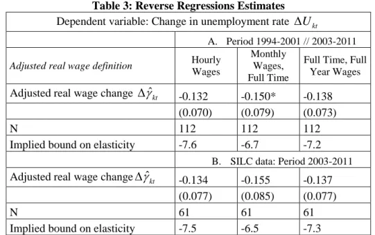
Following among others Friedman and Schwartz (1982), we also estimate the “errors-in-variables bounds” of Gini (1921) and Frisch (1934).32
These bounds can be obtained by reversing the direction of the regression, which implies regressing changes in the unemployment rates on changes in wages. If measurement errors are classical, the original regression gives a downward biased estimate of the true coefficient (in absolute value). In contrast, the inverse of the OLS coefficient of the reverse regression gives an upward biased estimate, thus bracketing the true value. Table 3 displays the reverse regression estimates. The bounds confirm that adjusted real wage changes are pro-cyclical, but they are quite large: the reverse regressions provide an upper bound from −7 to −6, while the
corresponding original regression estimates were close to −0.7.33
An important caveat is that the previous bounds are only valid under the assumptions of classical measurement errors, which is open to question. Papers by Bound and Krueger (1991) and
32
See Klepper and Leamer (1984) for a generalisation to multivariate regressions and Erickson (1993) for a discussion of the important case where measurements errors are correlated.
33
As discussed by Hausman (2001), the width of these bounds is proportional to the
R
2of both the original andreverse regressions (where time fixed effects have been partialled out), which are identical. If
ˆ
is the OLS estimate of the coefficient original regression and
ˆ
invis the estimate obtained from the reverse regression, the bounds are such that
ˆ ˆ/ inv R2. In our case, theR
2is 0.08, which is relatively low.20 Black, Berger and Scott (2000) have documented negative correlations between measurement errors and true values in survey data. As discussed by Kim and Solon (2005), if measurement errors are mean-reverting, our estimates of wage cyclicality are downward biased. Unfortunately, in the absence of any validation study for ECHP or SILC data, we cannot assess how specific patterns of
measurement errors might influence the results. However, the fact that we obtain larger estimates in countries where labour income data were collected from administrative record is consistent with the presence of a downward bias in estimates using survey data. This suggests that the ‘true’ cyclicality of wages might be even larger than the one reported here.
Did the Cyclicality Change during the Great Recession?
Until this point, we have constrained the elasticity of the adjusted real wage growth to be similar before and during the Great Recession. We next investigate whether we find a different response of wages during this period. We first examine the residuals of the aggregate data and the data adjusted for composition effects after 2008 in Figure 3c and 3d. As for the overall period, while the correlation between wages and unemployment is positive in the aggregate data, there is a clear negative correlation during the Great Recession in the corrected data.
In panels A and B of Table 4, we formally test for a structural break in wage adjustment after 2008 with the following model 34:
1 2 2008
ˆ
kt tU
ktU e
kt tu
kt
34With at most 15 years in our sample, our time dimension is rather limited, so we do not perform structural break tests with an unknown break date.
21 where
e
t2008is an indicator function equal to one after 2008 and zero otherwise. The estimation results for 1994-2011 in Panel A where the data come from the ECHP and SILC panels provide no evidence that wage cyclicality varied in a significant way between the two periods.In Panel B, we restrict our sample to SILC data to get a more homogenous sample which
provides estimates using only the 2003-2011 period. The results indicate a negative coefficient for
2 while the coefficient of
1 is small or positive, which is not statistically significant, suggesting a larger response during the Great Recession than in 2003-2007.We conclude by providing a simple quantitative estimate of the importance of composition effects on average wages during the Great Recession. An intuitive way to assess the importance of composition effects is to estimate the counterfactual changes in average wage that would have been observed in 2011 had the composition of the labour force remained as it was in 2008. We estimate the following decomposition:
11 08 11 11
(
08)
11(Z )
08 08w
w
w
w Z
w
w
where
w
t is the average real wage observed in year t andw Z
t(
t')
is the counterfactual wage that would have been observed int
had the distribution of characteristicsZ
( , )
X
of employees remained as in periodt
. The term on the left side captures composition effects and reflects the changes in average real labour price that would have been observed in 2011 if the distribution of characteristics had become similar to that of 2008. The second term in the brackets captures price22 had the composition of the labour force remained constant at the 2008 level. To control for changes in composition, we use the reweighting approach proposed by DiNardo et al. (1996).35
Table 5 shows that composition effects were substantial and tend to be positive across all countries. Composition effects were particularly large in Belgium, Italy, France and Spain, which experienced the largest unemployment increase. They were quite low in Austria and Finland, where unemployment did not change much. Figure 4 represents graphically each element of the
decomposition on the unemployment change. While changes in observed average wages are weakly correlated with unemployment, changes in real wages net of composition effects are proportional to the unemployment change across countries.36
Overall, there are two main lessons from the results in this section. First, consistent with the previous literature, controlling for composition effects dramatically influences the estimated elasticity of wages. Once composition effects are accounted for, we find a strong response of real wage growth to unemployment. These findings confirm the conclusion of previous works using longitudinal micro data. Our estimated elasticities are remarkably in line with, although slightly lower, existing estimates in the literature.37
35We calculate weights for 24 groups of education and experience interacted with sex such that the reweighted
distribution in a given year is equal to that of the reference year. The “counterfactual” average wage is then simply obtained by using these weights.
36 The result is similar when excluding Spain from the sample, as demonstrated by Figure A1 in the Appendix.
37 The literature reports elasticities between −0.7 and −1.7 for the US (Solon et al., 1994) and −1.7 and −2.0 for
the UK (Devereux and Hart, 2006). For Eurozone countries, Anger (2011) reports elasticities from -0.8 to -1.7 for Germany, Verdugo (2013) finds −1.5 for France, Carneiro et al. (2012) find −1.6 to −2.5 for Portugal, Peng and Siebert (2008) find −1.4 to −3 for Italy, while de la Roca (2014) finds −0.4 for Spain. Most papers use a model similar to that of Eq. (1), but there are sometimes important differences in the sample construction and the unemployment measure used to estimate the model that must be taken into account to interpret the results. See Anger (2011) for a detailed discussion.
23 Second, there is no evidence that real wages were less cyclical during the Great Recession. On the contrary, our estimates indicate a substantial response of adjusted real wage growth to the
downturn in countries most affected by the crisis.
Testing for Heterogeneity in the Cyclical Adjustment of Wages
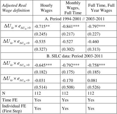
Following Swanson (2007), we use the richness of individual data to document heterogeneities in the cyclical adjustment of wages. We start by estimating a more flexible model allowing for a different response of the adjusted real wage growth to unemployment increases and decreases as in Martins (2007). The model is the following:
0 0
ˆ
kt kt kt tU e
kt UU e
kt Uu
kt
where
is the elasticity of log real wage net change of composition effects to unemployment increase and
is the elasticity to an unemployment decrease.The results in panel A of Table 6 indicate that there are significant differences in the response of real wage growth over the cycle. We obtain a much larger coefficient in response to unemployment increases than to decreases. In panel B, where the estimation period is much shorter, we find no response to unemployment decreases, while there is a strong procyclicality to unemployment increases. However, these differences should be interpreted with caution. As the standard errors of these estimates tend to be quite large, we can never reject formally the hypothesis of equality across these coefficients.
Second, we examine whether there are important differences in wage cyclicality across skill levels. In Table 7, we estimate separate models depending on the initial rank in the wage distribution of an individual when he or she is observed for the first time in the sample. The results point to significant variations between groups. The cyclicality of wage growth is much larger for those observed initially with wages below the first percentile (−0.9) than between the first quartile and the median (−0.3).
Overall, an important lesson from Tables 6 and 7 is that there are significant differences in wage cyclicality between phases of the cycle and workers. That we obtain a higher pro-cyclicality of
24 wages for low wage workers is consistent with evidence from Swanson (2007) for US data. Our results are nevertheless not always in line with the rest of the literature. The fact that wages tend to be more procyclical during downturns is consistent with evidence from Verdugo (2013) for France and Martins (2007) for Portugal but is in opposition with results from Font et al. (2015) for Spain and Shin and Shin (2008) for the US.
Next, we distinguish the response of wages between those changing employers and those remaining in the same job. The more important cyclicality of the wages of job changers has been underlined in the empirical literature (see, e.g., Devereux and Hart, 2006) and might reflect the existence of implicit contracts insuring workers remaining with the same employer from excessive income fluctuations (Beaudry and DiNardo, 1991). Focusing on males, we estimate two series of corrected wage indexes for stayers and shifters using the following model:
1
stay shift
ikt it i kt ikt kt ikt ikt
w
X
S
S
e
where
S
ikt is an indicator variable equal to one when an individual has changed employers during the year. In the second step, we regress the estimates of
ktstay and
ktshift on the unemployment change and level. The results of these estimates are provided in Table 8. As expected, job-changers exhibit a much higher level of cyclicality than job stayers: the procyclicality of wages growth of job changers is found to be the double of the one of stayers in Panel A. In any case, the fact that we find larger procyclicality of movers is in line with Devereux and Hart (2006) for the UK or Martins (2007) for PortugalIn panel B, where monthly wages are used, the differences are smaller. In addition, in both panels, as the standard errors are quite large, we cannot reject the hypothesis of equality of the coefficients across each type of workers.
25 As the unemployment dispersion is often large across regions and tends to widen during downturns,a key question is whether wages additionally react to the local economic shocks
(Blanchard and Katz, 1992; Blanchflower and Oswald, 1995). 38 Following recent work by Gregg et al. (2014) and Swanson (2007), we estimate whether real wages additionally respond to differences in the regional unemployment rate. We use the following first step model:
ikrt it i krt ikt
w X
e (3)where
krt varies across regionsr
within countriesk
. In the second step, we consider the model:ˆ
krt t NU
kt RU
k tru
kt
(4)where the composition adjusted regional average wage
ˆ
krtis used as a dependent variable and the regression include simultaneously the national (U
kt) and regional (U
krt) unemployment rates as covariates in the model.The results are reported in Table 9. Because the data do not contain information on regions for the Netherlands, we exclude this country from the sample.39 For comparison, Column 1 shows an estimate of the baseline model without the Netherlands in the sample. Columns 2 and 3 show estimates using, alternatively, the national or regional unemployment rate; the coefficient of the regional unemployment rate is negative but is measured quite imprecisely. When both rates are included in the model, as in Column 4, the elasticity to the regional unemployment is close to zero. In
38 In Spain, for example, in 2011, the unemployment rate was 31% in Andalusia but only 13% in the Basque
Country.
39 Regional boundaries in ECHP and SILC change in an important way between the two surveys. We have
matched these definitions with data from the European LFS and calculated regional unemployment rates corresponding to the specific definitions available in the panel data. See the appendix for details.
26 Column 5, we include country by year fixed effects, which absorb national level average variations in wages. Once again, the elasticity to regional unemployment is close to zero.
A potential issue is that our sample includes both large and small countries. The response to a regional shock may differ between the two, as it might be easier to move from the South to the North in a small country such as Belgium or Austria than in Italy or Spain. To explore this question, we estimate for each country a model including regional unemployment rate and time-fixed effects. For most countries, Table 10 shows that there is little evidence of an additional wage adjustment to regional unemployment. If anything, we obtain a positive coefficient in Austria and Belgium.
Overall, an important lesson from Table 9 and 10 is that differences in regional unemployment rate do not account much for cyclical wage variations once the effect the national unemployment rate has been accounted for. This result is consistent with recent work from Gregg et al. (2014) for the UK and Swanson (2007) for the US. This suggests that most the adjustment to regional disparities will rely on internal migration, as the average response of wages seems to be driven by national level trends.
Downward nominal wage rigidity during the Great Recession
IV.
In the previous model, real wages were used as a dependent variable, and as a result, the potential interactions between the adjustment of wages and inflation were not taken into account. Variations in the inflation level might have important consequences on the adjustment of real wages if nominal wages are rigid. In a low inflation environment, especially if inflation fluctuations are not
anticipated (Elsby, 2009), firms might find it difficult to adjust real wages downward because doing so implies decreasing the nominal wage (Tobin, 1972). In this section, we assess the evidence for downward nominal wage rigidity, particularly during the Great Recession when significant fluctuations in the inflation rate occurred. In order to focus on a more homogenous sample and for brevity, we concentrate on evidence from the SILC data. For comparison, the results obtained with the ECHP panel for the earlier periods are reproduced in the appendix in Tables A2 and A3.
Following the literature, we start by presenting visual evidence from the distribution of individual wage growth. To better capture rigidities, we exclude job changers and focus on full-time full-year workers to minimise measurement errors. Figure 5 presents a series of histograms of the
27 distribution of year-to-year changes in nominal wages in the SILC sample in 2009, during the Great Recession, and just before, in 2007.40 Such distribution directly depicts the share of wage changes that are negative and close to zero. For Portugal, because there was an important change in the data collection procedure in 2009, which makes the 2008-2009 changes unreliable, we use instead changes from the 2009-2010 period.41 As in Card and Hyslop (1997), the inflation rate of both periods is drawn using a vertical line, with a solid line for 2008 and a dashed line for 2009.
The first panel of Figure 5 represents the groups of countries for which income data were collected using administrative records, while countries in the second panel rely on information on income from household surveys. Consistent with Dickens et al. (2007), we find that these distributions have a number of characteristics in common but also notable differences. Four features stand out.
First, as highlighted in the previous literature, nominal wage decreases are not rare. Depending on country and year, approximately 20-40% of workers experienced nominal-wage cuts, which is strong evidence that nominal wages are not completely sticky for a large proportion of the workforce. In particular, data from France, Italy, the Netherlands and Finland, all collected from administrative records, show a high frequency of nominal wage reductions.
Second, consistent with the results in the previous section, measured year-to-year changes in individual wages have clearly responded to the Great Recession; for most countries, the distribution clearly shifted to the left in 2009. Table 11 reports the share of negative nominal and real wage changes from 2003 to 2011. Accordingly, the share of workers with negative nominal wage changes increased substantially in 2009 and 2010.
40 For scale reasons, the real wage changes have been censored at +/−0.4, and the masses at the upper and lower
extremes represent cumulative fractions.
41
Starting in 2008, most wages in Portugal were collected as the net of social contributions while previously gross wages were collected.
28 Third, even if negative nominal wage changes were relatively frequent, inflation nonetheless played an important role in real adjustments, as a substantial share of nominal increases are below 2-3%. For example, while the share of workers with negative nominal changes decreased from 2009 to 2010 by 3 percentage points in France, the share of workers with negative real change increased by 11 points, as inflation rebounded in 2010 with respect to 2009. A comparison with similar figures
obtained from administrative data for the UK reported in Elsby et al. (forthcoming) in the last two columns is also noteworthy: negative nominal wage changes were less frequent in the UK than in France or Finland. In contrast, negative real wage changes were substantially larger in the UK, particularly in 2010.
Fourth, evidence for the existence of a spike at zero before and during the Great Recession is mixed. A spike is visually discernible in Spain and, to a lesser extent, in Austria, with an average share of 8% and 3% of wage freezes over the 2004-2010 period, respectively. In countries using payroll data, less than 1% of individuals have an identical wage over two years.
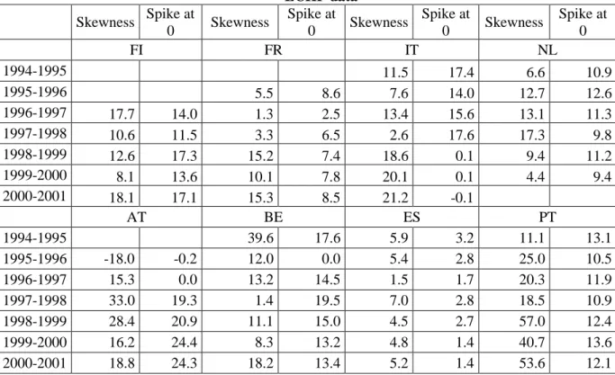
To examine more formally how these distributions evolve over the cycle, we compute distributional statistics for each country and year that aim to capture the type of distributional asymmetries often highlighted in the literature on downward nominal wage rigidities.42 First, following Guvenen et al. (2014), we estimate the evolution of the skewness of the distribution using “Kelley’s measure of skewness”, which relies on the quantiles of the distribution and is thus robust to outliers. This statistics measure the changes in an excess mass to the right and is defined as the relative difference between the upper and lower tail inequalities: (P90-P50 – P50-P10)/(P90-P10). Second, to
42
For a different approach that adopts a fully parametric specification of the wage change process, see Altonji and Devereux (2000) and Bauer et al. (2007).
29 assess the importance of the peak at zero, following Kurmann et al. (2014), we estimate the following statistics:
(0.005)
( 0.005)
(2
0.005)
(2
0.005)
kt kt kt
sp
F
F
F
median
F
median
.This statistic measures the difference between the mass around zero at the left of the median and the corresponding mass to the right of the median. If the distribution is symmetric, these two statistics are equal to zero. They are positive when the distribution is characterised by the type of asymmetries associated with downward wage rigidities.
These statistics are reported for each country in Table 12, while Table 13 systematically investigates their correlation with the cycle. For most countries, there is a clear decrease in the skewness of the wage change distribution during the Great Recession; regression results in Table 13 show that the skewness of the distribution is negatively related to increases in the unemployment rate, both in countries using administrative and in those using survey data. This implies that during the Great Recession, the probability of a substantial negative wage change increased markedly while the probability of large wage increases decreased.
The evidence is less clear with respect to the spike at zero. Table 12 shows that there are substantial disparities between Spain and Austria, where some evidence of a spike at zero is discernible, and other countries, where this statistic is quite small and varies only marginally. If anything, the regression in Table 13 indicates a positive correlation in countries with administrative data but a negative correlation in countries using survey data. Interestingly, similar statistics for ECHP reported in Table A3 for earlier periods show stronger evidence of peaks at zero for most countries.
Such systematic variations between countries using administrative records and countries using survey data suggest that differences in data quality complicate cross-country comparisons. Among other examples, large negative variations greater than −0.1 are quite rare in countries using administrative data (less than 10% in France, Finland and Italy and 4% in the Netherlands) but are observed more frequently in countries using survey data (approximately 20% in Spain and Austria). We also find significant differences in the autocovariance of individual wage changes in the SILC data. Following Dickens et al. (2007), we show in the appendix that, under some hypotheses, the more
30 errors that are present in a dataset, the more negative the auto-covariance of wage changes should be.43 The results in Appendix Table A4 indicate that countries using administrative data tend to have a much lower auto-covariance than those using survey data. In particular, the auto-covariance is ten times larger in Spain and Austria, which use survey data, than in the Netherland and Finland, which rely on administrative data. Somewhat surprisingly, the auto-covariance is found to be relatively small in Portugal.
Before concluding this section, it is important to bear in mind that the previous results were obtained using total wages. Unfortunately, we are not able to distinguish in our data the base wage, which might be much more downward rigid. Recent work by Carneiro et al. (2014) for Portugal using administrative data points to the existence of significant rigidities in the base wage during the Great Recession. In particular, they report a share of 30% of base wage freezes in 2013 against only 5% in 2008. Such rigidity of the base wage is consistent with results from Swanson (2007) for the US who remarks that the base wage is not cyclical.
The exceptional severity of the recent downturn in Portugal might also explain the large share of base-wage freezes reported by Carneiro et al. (2014), as wages have not been found particularly rigid in Portugal in previous work from the same authors.44 Differences in the quality of the data might also play a role, but this cannot be the whole explanation. As highlighted above, we find little evidence of wage freezes for four European countries using administrative data during the Great Recession in our sample, which is consistent with other recent studies using administrative data for
43 Such a conclusion is valid under the hypothesis that the “true” auto-covariance of wage change does not vary
too much across countries and over time.
44 Using the same administrative data, Carneiro et al. (2012) report an even larger cyclicality of wages in
Portugal than in the US or the UK in the pre-Great Recession period with an elasticity of real wages to the cycle of −1.6 to −2.5 over the period 1986-2005.
31 France (Audenaert et al., 2014), the UK (Elsby et al., forthcoming), Ireland (Doris et al., 2012), and the US (Kurmann et al., 2014).
Discussion
V.
Using individual level data for the Eurozone before and during the Great Recession, we have investigated the relationship between real wages and change in unemployment rates. We found that composition effects hide the significant correlation between real wage changes at the worker level and the business cycle. With individual data, we estimate an elasticity of real wage growth, net of
composition effects, to unemployment rate changes between −0.6 and −1. We also find a substantially larger elasticity for job changers and workers at the top of the wage distribution. Finally, we do not find evidence of an additional correlation of wages to region-specific changes in unemployment.
Consistent with these findings, we find that composition effects were large during the Great Recession and that they potentially explain most of the stagnation or increases in average wages observed in the aggregate data from 2008 to 2010 in countries most affected by an unemployment increase. At the worker level, the data indicate much larger wage adjustments during the downturn in countries most affected by the crisis.
The results in this paper have several implications. First, they confirm that the evolution of the aggregate real wage series is partially misleading. International comparisons of wage adjustments based on aggregate data must be interpreted with caution when there are simultaneously large differences in unemployment change across countries.
The results also suggest that the creation of a wage index that accounts for composition effects would have a substantial payoff. Clearly, this index would be most useful if it is sufficiently
homogenous across countries and could be updated relatively rapidly. One important finding is that simple regression techniques with cross-section data to control for composition effects might account for a large share of the compositional biases.
Finally, to assess differences in wage rigidity across countries, the availability of homogenous high quality administrative data on wages for a larger set of countries would also be desirable. While half of the countries in our sample used administrative data, the other half relied on household surveys,
32 complicating cross-country comparisons. A generalization of the use of administrative data in the SILC panel would be a great asset for future research on the European economy.