Surface wave tomography of the Barents Sea and surrounding regions

(1)

HAL Id: hal-00311703

https://hal.archives-ouvertes.fr/hal-00311703

Submitted on 5 Jul 2017

HAL is a multi-disciplinary open access

archive for the deposit and dissemination of

sci-entific research documents, whether they are

pub-lished or not. The documents may come from

teaching and research institutions in France or

abroad, or from public or private research centers.

L’archive ouverte pluridisciplinaire HAL, est

destinée au dépôt et à la diffusion de documents

scientifiques de niveau recherche, publiés ou non,

émanant des établissements d’enseignement et de

recherche français ou étrangers, des laboratoires

publics ou privés.

Surface wave tomography of the Barents Sea and

surrounding regions

Anatoli L. Levshin, Johannes Schweitzer, Christian Weidle, Nikolai M.

Shapiro, Michael H. Ritzwoller

To cite this version:

Anatoli L. Levshin, Johannes Schweitzer, Christian Weidle, Nikolai M. Shapiro, Michael H. Ritzwoller.

Surface wave tomography of the Barents Sea and surrounding regions. Geophysical Journal

Interna-tional, Oxford University Press (OUP), 2007, 170 (1), pp.441-459. �10.1111/j.1365-246X.2006.03285.x�.

�hal-00311703�

(2)

GJI

T

ectonics

and

geo

dynamics

Surface wave tomography of the Barents Sea and surrounding regions

Anatoli L. Levshin,

1 Johannes Schweitzer,

2 Christian Weidle,

3 Nikolai M. Shapiro

1 ,4

and Michael H. Ritzwoller

1

1_{Department of Physics, University of Colorado at Boulder, Boulder, CO 80309, USA. E-mail: levshin@tinker.colorado.edu} 2_{NORSAR, POB 53, NO-2027 Kjeller, Norway}

3_{Institutt for geofag, Universitetet i Oslo, Norway} 4_{Institute de Physique du Globe, CNRS, Paris, France}

Accepted 2006 November 3. Received 2006 October 20; in original form 2006 April 18

S U M M A R Y

The goal of this study is to refine knowledge of the structure and tectonic history of the

Euro-pean Arctic using the combination of all available seismological surface wave data, including

historical data that were not used before for this purpose. We demonstrate how the improved

data coverage leads to better depth and spatial resolution of the seismological model and

dis-covery of intriguing features of upper-mantle structure. To improve the surface wave data set

in the European Arctic, we extensively searched for broad-band data from stations in the area

from the beginning of the 1970s until 2005. We were able to retrieve surface wave observations

from regional data archives in Norway, Finland, Denmark and Russia in addition to data from

the data centres of IRIS and GEOFON. Rayleigh and Love wave group velocity measurements

between 10 and 150 s period were combined with existing data provided by the University of

Colorado at Boulder. This new data set was inverted for maps showing the 2-D group-velocity

distribution of Love and Rayleigh waves for specific periods. Using Monte Carlo inversion,

we constructed a new 3-D shear velocity model of the crust and upper mantle beneath the

European Arctic which provides higher resolution and accuracy than previous models. A new

crustal model of the Barents Sea and surrounding areas, published recently by a collaboration

between the University of Oslo, NORSAR and the USGS, constrains the 3-D inversion of the

surface wave data in the shallow lithosphere. The new 3-D model, BARMOD, reveals

sub-stantial variations in shear wave speeds in the upper mantle across the region with a nominal

resolution of 1

◦

× 1

◦

. Of particular note are clarified images of the mantle expression of the

continent-ocean transition in the Norwegian Sea and a deep, high wave speed lithospheric

root beneath the Eastern Barents Sea, which presumably is the remnant of several Palaeozoic

collisions.

Key words: crustal structure, European Arctic, lithosphere, surface waves, tomography,

upper mantle.

1 I N T R O D U C T I O N

The goal of this study is to refine our knowledge of the structure and

tectonic history of the European Arctic by combining all available

seismological surface wave data, including historical data that were

not used before for this purpose. This work should be considered in

the context of on-going and planned developments in studying the

Earth’s polar regions, particularly during and following the

Interna-tional Polar Year of 2007–2008. We demonstrate how the

improve-ment in data coverage leads to better depth and spatial resolution

of the seismological model and the discovery of intriguing features

of the upper mantle. The rapid growth of seismic observations in

the Arctic in the coming years will provide further opportunities for

extending and refining this model.

The structure of the crust and upper mantle beneath the European

Arctic, and the Barents Sea especially, has been the subject of

spe-cial interest among Earth scientists in the recent years (e.g. Vorren

et al. 1990; Gudlaugsson et al. 1998; Breivik et al. 1999, 2002;

Artyushkov 2004, 2005; Mann et al. 2004; Ebbing et al. 2005).

This relatively small region includes a complex of diverse tectonic

features such as the deep ocean, a continental margin, a mid-ocean

ridge, an ancient shield, and a continental shelf with one of most

prominent sedimentary basins in the world (Fig. 1a). The upper

crust of the eastern Barents Sea shelf is relatively well studied, as

this area is considered to have high oil and gas resources. The

tec-tonic history of the basin, however, and its relation to the structure

of the underlying mantle remains poorly understood. In addition,

knowledge of the deep structure of this region is important for

(3)

(a)

300˚ 320˚ 340˚ 0˚ 20˚ 40˚ _60˚ 80˚ 100˚ 120˚ 140˚ 160˚ 60˚ 60˚ 80˚ 80˚

(b)

20˚ 40˚ 60˚ 80˚ 65˚ 70˚ 75˚ 20˚ 40˚ 60˚ 80˚ 65˚ 70˚ 75˚ 20˚ 40˚ 60˚ 80˚ 65˚ 70˚ 75˚ 20˚ 40˚ 60˚ 80˚ 65˚ 70˚ 75˚ 20˚ 40˚ 60˚ 80˚ 65˚ 70˚ 75˚ 20˚ 40˚ 60˚ 80˚ 65˚ 70˚ 75˚ 20˚ 40˚ 60˚ 80˚ 65˚ 70˚ 75˚ 20˚ 40˚ 60˚ 80˚ 65˚ 70˚ 75˚ ? ?

East Barents Basin

North Atlantic ridge

Svalbard Baltic Shield N ovaya Z em lya Pechora Basin Caledonian Timanian Uralian Barents Sea Kara Sea

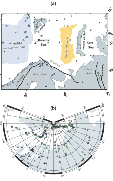
Figure 1. (a) The map shows the most relevant tectonic features discussed in the text. Blue shaded regions depict the north Atlantic oceanic domain, outlining

the continent–ocean boundary in the European Arctic and the Norwegian Sea. The yellow shaded area in the East Barents Sea marks sediment thicknesses larger than 9 km in the East Barents Sea basin, after Johansen et al. (1992). Note that the geometry in the northern part of the basin is uncertain as indicated by question marks. The mid-Atlantic ridge is traced by the epicentres (green stars) and stations used in this study are displayed by blue triangles. (b) The map shows the location of the seismic stations (blue triangles) and events used in this study (see also Table 1). The epicentres of the earthquakes are shown by green stars, explosions as green circles.

monitoring seismic activity within the region, which includes the

Soviet nuclear test site at Novaya Zemlya.

Kremenetskaya et al. (2001) published a 1-D velocity model for

the wider Barents Sea region. Hicks et al. (2004) demonstrated

that the 1-D model called Barey (Schweitzer & Kennett 2002, cf.

Fig. 12), a slightly modified version of the Barents Sea model

by Kremenetskaya et al. (2001) on top of model ak135 (Kennett

et al. 1995), is superior to other models for locating seismic

events in the wider Barents Sea region. However, because of

the known differences in the crustal structure, any 1-D model

will have its limits in describing the velocity structure of the

region.

The investigation of velocities in crust and uppermost

man-tle below the Barents Sea with surface waves started in 1970s.

Calcagnile & Panza (1978) measured the interstation phase

veloc-ities of Rayleigh waves across the western part of the Barents Sea

between stations KBS (Svalbard) and KRK (Norway) and inverted

these measurements for an average crust and upper-mantle structure.

McCowan et al. (1978) measured intersource phase velocities of

Rayleigh waves from nuclear tests at two Soviet test sites at Novaya

(4)

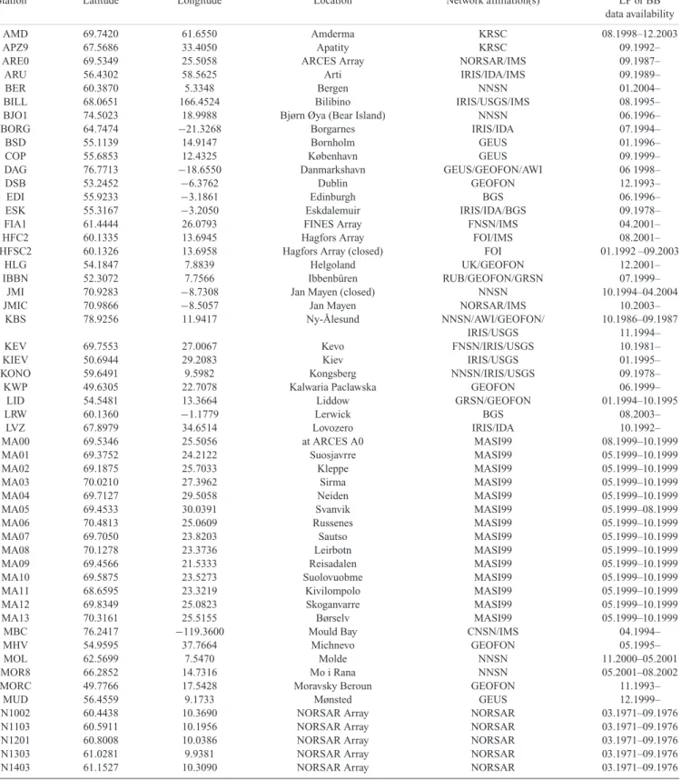
Table 1. List of seismic stations from which surface wave data were retrieved to increase the ray coverage in the Barents Sea and surrounding

regions (see also Fig. 1). The abbreviations in the network-affiliation column stand for: AWI—Alfred-Wegener-Institute for Polar and Marine Re-search, BGS—British Geological Service, CNSN—Canadian National Seismograph Network, FNSN—Finish National Network (University in Helsinki), FOI—Totalf¨orsvarets forskningsinstitut (Sweden), GEUS—Danmarks og Grønlands Geologiske Undersøgelse, GRSN—German Regional Seismic Net-work, IDA—International Deployment of Accelerometers, IMS—International Monitoring System, IRIS—Incorporated Research Institutions for Seismology, KRSC—Kola Regional Seismological Center, MASI99—Temporal net of seismic stations in Finmark operated by NORSAR and the University of Potsdam (Germany) (Schweitzer 1999), NNSN—Norwegian National Seismic Network (University in Bergen), RUB—Ruhr University Bochum, UK—University in Kiel, and USGS—US Geological Survey. The data availability for some of the stations may be longer than known to us.

Station Latitude Longitude Location Network affiliation(s) LP or BB

data availability

AMD 69.7420 61.6550 Amderma KRSC 08.1998–12.2003

APZ9 67.5686 33.4050 Apatity KRSC 09.1992–

ARE0 69.5349 25.5058 ARCES Array NORSAR/IMS 09.1987–

ARU 56.4302 58.5625 Arti IRIS/IDA/IMS 09.1989–

BER 60.3870 5.3348 Bergen NNSN 01.2004–

BILL 68.0651 166.4524 Bilibino IRIS/USGS/IMS 08.1995–

BJO1 74.5023 18.9988 Bjørn Øya (Bear Island) NNSN 06.1996–

BORG 64.7474 −21.3268 Borgarnes IRIS/IDA 07.1994–

BSD 55.1139 14.9147 Bornholm GEUS 01.1996–

COP 55.6853 12.4325 København GEUS 09.1999–

DAG 76.7713 −18.6550 Danmarkshavn GEUS/GEOFON/AWI 06 1998–

DSB 53.2452 −6.3762 Dublin GEOFON 12.1993–

EDI 55.9233 −3.1861 Edinburgh BGS 06.1996–

ESK 55.3167 −3.2050 Eskdalemuir IRIS/IDA/BGS 09.1978–

FIA1 61.4444 26.0793 FINES Array FNSN/IMS 04.2001–

HFC2 60.1335 13.6945 Hagfors Array FOI/IMS 08.2001–

HFSC2 60.1326 13.6958 Hagfors Array (closed) FOI 01.1992 –09.2003

HLG 54.1847 7.8839 Helgoland UK/GEOFON 12.2001–

IBBN 52.3072 7.7566 Ibbenb¨uren RUB/GEOFON/GRSN 07.1999–

JMI 70.9283 −8.7308 Jan Mayen (closed) NNSN 10.1994–04.2004

JMIC 70.9866 −8.5057 Jan Mayen NORSAR/IMS 10.2003–

KBS 78.9256 11.9417 Ny-Ålesund NNSN/AWI/GEOFON/ 10.1986–09.1987

IRIS/USGS 11.1994–

KEV 69.7553 27.0067 Kevo FNSN/IRIS/USGS 10.1981–

KIEV 50.6944 29.2083 Kiev IRIS/USGS 01.1995–

KONO 59.6491 9.5982 Kongsberg NNSN/IRIS/USGS 09.1978–

KWP 49.6305 22.7078 Kalwaria Paclawska GEOFON 06.1999–

LID 54.5481 13.3664 Liddow GRSN/GEOFON 01.1994–10.1995

LRW 60.1360 −1.1779 Lerwick BGS 08.2003–

LVZ 67.8979 34.6514 Lovozero IRIS/IDA 10.1992–

MA00 69.5346 25.5056 at ARCES A0 MASI99 08.1999–10.1999

MA01 69.3752 24.2122 Suosjavrre MASI99 05.1999–10.1999

MA02 69.1875 25.7033 Kleppe MASI99 05.1999–10.1999

MA03 70.0210 27.3962 Sirma MASI99 05.1999–10.1999

MA04 69.7127 29.5058 Neiden MASI99 05.1999–10.1999

MA05 69.4533 30.0391 Svanvik MASI99 05.1999–08.1999

MA06 70.4813 25.0609 Russenes MASI99 05.1999–10.1999

MA07 69.7050 23.8203 Sautso MASI99 05.1999–10.1999

MA08 70.1278 23.3736 Leirbotn MASI99 05.1999–10.1999

MA09 69.4566 21.5333 Reisadalen MASI99 05.1999–10.1999

MA10 69.5875 23.5273 Suolovuobme MASI99 05.1999–10.1999

MA11 68.6595 23.3219 Kivilompolo MASI99 05.1999–10.1999

MA12 69.8349 25.0823 Skoganvarre MASI99 05.1999–10.1999

MA13 70.3161 25.5155 Børselv MASI99 05.1999–10.1999

MBC 76.2417 −119.3600 Mould Bay CNSN/IMS 04.1994–

MHV 54.9595 37.7664 Michnevo GEOFON 05.1995–

MOL 62.5699 7.5470 Molde NNSN 11.2000–05.2001

MOR8 66.2852 14.7316 Mo i Rana NNSN 05.2001–08.2002

MORC 49.7766 17.5428 Moravsky Beroun GEOFON 11.1993–

MUD 56.4559 9.1733 Mønsted GEUS 12.1999–

N1002 60.4438 10.3690 NORSAR Array NORSAR 03.1971–09.1976

(5)

Table 1. (Continued.)

Station Latitude Longitude Location Network affiliation(s) LP or BB

data availability

NAO01 60.8442 10.8865 NORSAR Array NORSAR/IMS 03.1971–

NB201 61.0495 11.2939 NORSAR Array NORSAR/IMS 03.1971–

NB302 60.9158 11.3309 NORSAR Array NORSAR 03.1971–09.1976

NBO00 61.0307 10.7774 NORSAR Array NORSAR/IMS 03.1971–

NC204 61.2759 10.7629 NORSAR Array NORSAR/IMS 03.1971–

NC503 60.9075 11.7981 NORSAR Array NORSAR 03.1971–09.1976

NCO00 61.3374 10.5854 NORSAR Array NORSAR 03.1971–09.1976

NOR 81.6000 −16.6833 Nord GEUS/GEOFON 08.2002–

NRE0 60.7352 11.5414 NORES Array NORSAR 10.1984–06.2002

NRIL 69.5049 88.4414 Norilsk IRIS/IDA/IMS 12.1992 –

NSS 64.5307 11.9673 Namsos NNSN 10.2001–

OBN 55.1138 36.5687 Obninsk IRIS/IDA 09.1988–

PUL 59.7670 30.3170 Pulkovo GEOFON 05.1995–

RGN 54.5477 13.3214 R¨ugen GRSN/GEOFON 12.1995–

RUE 52.4759 13.7800 R¨udersdorf GRSN/GEOFON 01.2000–

RUND 60.4135 5.3672 Rundemannen NNSN 03.1997–03.2003

SCO 70.4830 −21.9500 Ittoqqortoormiit (Scoresbysund) GEUS 05.1999–

STU 48.7719 9.1950 Stuttgart GEOFON/GRSN 04.1994–

SUMG 72.5763 −38.4540 Summit Camp GEOFON 06.2002–

SUW 54.0125 23.1808 Suwalki GEOFON 11.1995–

TIXI 71.6490 128.8665 Tiksi IRIS/USGS/IMS 08.1995–

TRO 69.6345 18.9077 Tromsø NNSN 03.2003–

TRTE 58.3786 26.7205 Tartu GEOFON 06.1996–04.2003

VSU 58.4620 26.7347 Vasula GEOFON 04.2003–

WLF 49.6646 6.1526 Walferdange GEOFON 03.1994–

YAK 62.0308 129.6812 Yakutsk IRIS/USGS/IMS 09.1993–

Zemlya recorded by the ALPHA array in Alaska to get the

struc-tural model under Novaya Zemlya. After the NORSAR array had

been installed in Southern Norway, Bungum & Capon (1974) and

Levshin & Berteussen (1979) observed mutlipathing of Rayleigh

waves due to major tectonic boundaries in and around the

Euro-pean Arctic. Levshin & Berteussen (1979) investigated in detail

sur-face wave observations from nuclear explosions on Novaya Zemlya

and were able to derive a mean velocity model for the Barents Sea

part of the path between Novaya Zemlya and NORSAR based on

group and phase velocity observations. Chan & Mitchell (1985)

and Egorkin et al. (1988) obtained average crustal models along

several profiles crossing the Barents Sea using analogue records

of earthquakes from seismic stations KHE (Franz Josef Land),

APA (Kola Peninsula), KBS, KEV (Finland) and digital NORSAR

data.

A surface wave tomography has been published for the Arctic,

which shows the large scale velocity features in the larger Barents

Sea region (Levshin et al. 2001; Shapiro & Ritzwoller 2002). This

tomography based on group-velocity measurements of Love and

Rayleigh waves, which had been compiled globally over the years

at the University of Colorado. Recently, Pasyanos (2005) published

group-velocity maps for Eurasia and the European Arctic, which

show very similar large scale features. He used the University of

Colorado data set and extended it by his own surface wave

ob-servations. However, he could not achieve higher resolution in the

European Arctic due to the lack of additional regional surface wave

observations.

Thus, all published global and regional tomographic models have

poor resolution in the European Arctic due to the small number of

seismic stations, relatively low regional seismicity, and limited a

priori knowledge of the crustal structure. During the past decade,

several new seismic stations were permanently or temporarily

in-stalled in and around this region. Many of the data from these stations

are not easily accessible via the international data centres but only

by direct request to the network operators. We have systematically

searched during this study for additional broad-band waveform data

observed at seismic stations and arrays in the area of interest from

the early 1970s until 2005 (Levshin et al. 2005a,b). These newly

analysed surface wave data are combined with a subset of the data

from the University of Colorado (CU-Boulder). The resulting data

set of Love- and Rayleigh-wave observations, for waves traversing

the wider Barents Sea area, has a much higher path density than

achieved in previous studies and thereby a higher resolution of

lat-eral heterogeneities in seismic velocities.

(6)

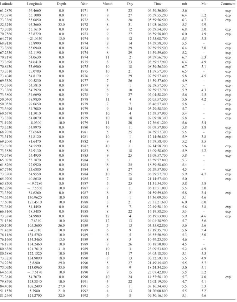
Table 2. List with source parameters of the seismic events newly investigated during this study for measuring the group velocities of surface waves. A map

with the event locations is shown on Fig. 1. All nuclear explosions are marked as ‘exp’.

Latitude Longitude Depth Year Month Day Time mb Ms Comment

61.2870 56.4660 0.0 1971 3 23 06:59:56.000 5.6 – exp 73.3870 55.1000 0.0 1971 9 27 05:59:55.200 6.4 5.2 exp 73.3360 55.0850 0.0 1972 8 28 05:59:56.500 6.3 4.7 exp 52.3240 95.3660 33.0 1972 8 31 14:03:16.300 5.5 4.9 73.3020 55.1610 0.0 1973 9 12 06:59:54.300 6.8 5.0 exp 70.7560 53.8720 0.0 1973 9 27 06:59:58.000 6.0 4.9 exp 64.7710 −21.0450 13.0 1974 6 12 17:55:08.700 5.5 5.3 68.9130 75.8990 0.0 1974 8 14 14:59:58.300 5.5 – exp 73.3660 55.0940 0.0 1974 8 29 09:59:55.500 6.4 5.0 exp 67.2330 62.1190 0.0 1974 8 29 14:59:59.600 5.2 – exp 70.8170 54.0630 0.0 1974 11 2 04:59:56.700 6.7 5.3 exp 73.3690 54.6410 0.0 1975 8 23 08:59:57.900 6.4 4.9 exp 70.8430 53.6900 0.0 1975 10 18 08:59:56.300 6.7 5.1 exp 73.3510 55.0780 0.0 1975 10 21 11:59:57.300 6.5 – exp 73.4040 54.8170 0.0 1976 9 29 02:59:57.400 5.8 4.5 exp 69.5320 90.5830 0.0 1977 7 26 16:59:57.600 4.9 – exp 73.3760 54.5810 0.0 1977 9 1 02:59:57.500 5.7 – exp 73.3360 54.7920 0.0 1978 8 10 07:59:57.700 5.9 4.3 exp 73.3800 54.6690 0.0 1978 9 27 02:04:58.200 5.6 4.5 exp 50.0460 78.9830 0.0 1978 11 4 05:05:57.500 5.6 4.2 exp 50.0530 79.0650 0.0 1979 7 7 03:46:57.400 5.8 – exp 73.3690 54.7080 0.0 1979 9 24 03:29:58.300 5.7 – exp 60.6770 71.5010 0.0 1979 10 4 15:59:57.900 5.4 – exp 73.3380 54.8070 0.0 1979 10 18 07:09:58.300 5.8 – exp 71.1920 −8.0300 10.0 1979 11 20 17:36:01.200 5.6 5.4 73.3530 54.9970 0.0 1980 10 11 07:09:57.000 5.8 3.8 exp 68.2050 53.6560 0.0 1981 5 25 04:59:57.300 5.5 – exp 73.3170 54.8120 0.0 1981 10 1 12:14:56.800 5.9 3.8 exp 69.2060 81.6470 0.0 1982 9 4 17:59:58.400 5.2 3.5 73.3920 54.5590 0.0 1982 10 11 07:14:58.200 5.6 3.6 exp 73.3830 54.9130 0.0 1983 8 18 16:09:58.600 5.9 4.2 exp 73.3480 54.4950 0.0 1983 9 25 13:09:57.700 5.8 – exp 65.0250 55.1870 0.0 1984 8 11 18:59:57.800 5.3 – 61.8760 72.0920 0.0 1984 8 25 18:59:58.600 5.4 – 67.7740 33.6880 0.0 1984 8 27 05:59:57.000 4.5 – exp 73.3700 54.9550 0.0 1984 10 25 06:29:57.700 5.9 4.7 exp 65.9700 40.8630 0.0 1985 7 18 21:14:57.400 5.0 – exp 63.8500 −19.7280 8.0 1987 5 25 11:31:54.300 5.8 5.8 82.2290 −17.5560 10.0 1987 7 11 06:15:51.000 5.5 5.0 73.3390 54.6260 0.0 1987 8 2 01:59:59.800 5.8 3.4 exp 74.6550 130.9620 10.0 1988 1 1 14:36:09.500 5.1 4.6 77.6010 125.4510 10.0 1988 3 21 23:31:21.600 6.0 6.0 73.3640 54.4450 0.0 1988 5 7 22:49:58.100 5.6 3.8 exp 66.3160 78.5480 0.0 1988 8 22 16:19:58.200 5.3 – exp 73.3870 54.9980 0.0 1988 12 4 05:19:53.000 5.9 4.6 exp 71.1340 −7.6340 10.0 1988 12 13 04:01:38.900 5.7 5.6 50.1030 105.3600 36.0 1989 5 13 03:35:02.800 5.6 5.6 71.4320 −4.3710 10.0 1989 6 9 12:19:35.700 5.6 5.4 76.1180 134.5780 10.0 1989 8 5 06:55:50.900 5.3 5.0 76.1660 134.3460 13.0 1989 8 5 10:49:23.300 4.6 – 76.1750 134.2460 10.0 1989 9 26 00:18:50.000 4.5 – 80.6380 121.7610 31.0 1989 10 3 23:09:53.800 5.2 4.9 80.5880 122.1320 10.0 1989 11 17 04:05:18.500 5.1 5.3 73.3250 134.9090 18.0 1990 3 13 00:32:59.100 5.5 4.9 74.2250 8.8280 29.0 1990 5 27 21:49:35.400 5.5 5.7 75.0920 113.0960 33.0 1990 6 9 18:24:34.200 5.0 5.1 64.6550 −17.6170 10.0 1990 9 15 23:07:42.800 5.5 5.2 73.3610 54.7070 0.0 1990 10 24 14:57:58.100 5.7 4.0 exp 79.8490 123.8840 10.0 1991 3 22 17:02:19.500 4.7 4.1 84.4010 108.2490 27.0 1991 6 11 07:16:34.400 5.5 5.3 51.1530 5.7980 21.0 1992 4 13 01:20:00.800 5.5 5.2 81.2460 121.2700 32.0 1992 6 8 09:30:16.100 5.1 4.6

(7)

64.7800 −17.5940 10.0 1992 9 26 05:45:50.600 5.5 5.4 86.9410 56.0730 10.0 1993 2 23 11:56:27.100 4.7 4.6 64.5780 −17.4820 9.0 1994 5 5 05:14:49.700 5.7 5.2 56.7610 117.9000 12.0 1994 8 21 15:55:59.200 5.8 5.8 78.3020 2.3020 10.0 1995 3 9 07:04:22.100 5.1 4.4 50.3720 89.9490 14.0 1995 6 22 01:01:19.000 5.5 5.2 51.9610 103.0990 12.0 1995 6 29 23:02:28.200 5.6 5.5 75.9840 6.9560 10.0 1995 10 4 09:17:30.200 5.1 4.9 56.1000 114.4950 22.0 1995 11 13 08:43:14.500 5.9 5.6 72.6440 3.4880 10.0 1995 12 8 07:41:12.700 5.2 5.2 75.8200 134.6190 10.0 1996 6 22 16:47:12.910 5.6 5.5 77.8600 7.5640 10.0 1996 8 20 00:11:00.340 5.3 5.0 77.7460 7.8770 10.0 1997 2 6 14:41:51.750 5.3 – 78.5100 125.5150 10.0 1997 4 16 08:42:27.550 4.8 4.3 78.4450 125.8210 10.0 1997 4 19 15:26:33.480 5.7 5.0 73.4170 7.9880 10.0 1997 10 6 21:13:10.380 5.0 – 79.8880 1.8560 10.0 1998 3 21 16:33:11.000 5.9 6.1 72.8260 129.5830 10.0 1998 8 23 09:59:02.970 4.5 – 86.2830 75.6090 10.0 1998 10 18 22:09:19.160 5.2 4.6 85.6410 86.1000 10.0 1999 2 1 04:52:40.810 5.1 4.7 85.7340 84.4390 10.0 1999 2 1 09:56:35.020 5.1 5.2 85.6050 85.8370 10.0 1999 2 1 11:55:15.070 4.5 – 85.5710 87.1410 10.0 1999 2 1 11:56:00.800 5.1 5.5 85.5730 87.0370 10.0 1999 2 19 19:10:00.540 5.1 5.0 86.2780 73.3940 10.0 1999 2 22 08:02:11.170 5.2 4.8 51.6040 104.8640 10.0 1999 2 25 18:58:29.400 5.9 5.5 85.6860 86.0340 10.0 1999 3 1 17:46:46.340 5.0 5.0 85.6920 84.7970 10.0 1999 3 13 01:26:33.540 5.3 5.1 85.6340 86.8190 10.0 1999 3 21 15:24:07.840 5.4 5.1 55.8960 110.2140 10.0 1999 3 21 16:16:02.200 5.5 5.7 85.6820 85.7360 10.0 1999 3 28 21:32:29.650 4.4 – 85.6440 86.2590 10.0 1999 3 28 21:33:44.090 5.0 5.1 85.6480 86.5310 10.0 1999 4 1 10:47:53.010 5.1 5.1 73.2150 6.6500 10.0 1999 4 13 02:09:22.270 5.0 4.7 85.6720 84.8300 10.0 1999 4 26 13:20:07.620 5.2 4.9 85.6320 86.1460 10.0 1999 5 18 20:20:16.060 5.1 5.3 85.6050 86.5260 10.0 1999 5 26 23:56:32.670 5.1 4.6 73.0170 5.1870 10.0 1999 6 7 16:10:33.630 5.3 5.4 73.0770 5.4530 10.0 1999 6 7 16:35:46.700 5.2 5.3 85.6040 83.7040 10.0 1999 6 11 23:54:52.000 5.1 4.5 85.6770 85.7720 10.0 1999 6 18 19:47:25.180 5.3 4.8 70.2800 −15.3510 10.0 1999 7 1 02:08:02.010 4.9 – 85.7410 83.2640 10.0 1999 7 8 19:25:10.520 5.0 4.6 72.2610 0.3960 10.0 1999 8 3 13:55:41.410 5.0 5.1 67.8630 34.3790 10.0 1999 8 17 04:44:35.950 4.6 – 79.2210 124.3970 10.0 1999 10 27 05:05:07.180 4.8 4.5 55.8300 110.0290 10.0 1999 12 21 11:00:48.870 5.5 5.0 80.6150 122.1300 10.0 1999 12 26 08:39:48.390 4.7 – 80.5820 122.2510 10.0 1999 12 30 06:46:55.250 4.7 4.4 79.8020 123.0760 10.0 2000 1 16 12:29:12.630 4.5 3.8 75.2710 10.1950 10.0 2000 2 3 15:53:12.960 5.5 5.0 79.8900 0.4380 10.0 2000 2 12 09:05:06.630 5.0 4.7 71.1900 −8.2630 10.0 2000 5 21 19:58:47.410 5.3 5.6 63.9660 −20.4870 10.0 2000 6 17 15:40:41.730 5.7 6.6 63.9800 −20.7580 10.0 2000 6 21 00:51:46.880 6.1 6.6 74.3330 146.9720 10.0 2000 7 10 04:17:36.830 4.6 3.9 78.9680 124.4680 10.0 2000 9 16 17:45:17.820 4.6 – 54.7070 94.9830 33.0 2000 10 27 08:08:53.540 5.6 5.3 81.5320 120.2790 27.3 2000 12 31 01:45:03.240 5.1 4.5 80.0380 122.7240 10.0 2001 4 8 02:59:03.880 4.5 – 80.4640 120.0940 10.0 2001 5 1 23:44:57.170 4.5 – 82.9330 117.5090 10.0 2001 5 30 15:19:04.350 4.7 – 72.6750 124.0160 61.5 2001 6 8 04:59:05.250 4.7 –

(8)

79.5140 4.1880 10.0 2001 7 16 14:09:29.240 5.0 4.5 80.8480 0.7680 10.0 2001 12 8 06:44:22.020 5.1 4.8 85.8580 27.6810 10.0 2002 5 3 11:19:20.320 4.1 – 86.0050 31.5950 10.0 2002 5 3 11:20:51.540 5.2 5.4 85.9720 31.1490 10.0 2002 5 3 15:33:34.880 5.1 5.1 86.2760 37.1770 10.0 2002 5 28 15:39:01.550 4.9 4.7 75.6340 143.7460 10.0 2002 6 4 00:05:07.170 4.8 – 84.0830 110.6900 10.0 2002 6 9 21:20:38.750 4.5 – 83.1360 −6.0780 10.0 2002 9 11 04:50:32.860 5.2 5.2 66.9380 −18.4560 10.0 2002 9 16 18:48:26.720 5.5 5.7 58.3110 −31.9460 10.0 2002 10 7 20:03:54.580 4.9 5.5 57.4490 −33.3440 10.0 2003 2 1 18:47:52.150 5.3 5.5 71.1220 −7.5770 10.0 2003 6 19 12:59:24.410 5.6 5.0 76.3720 23.2820 10.0 2003 7 4 07:16:44.720 5.7 5.1 73.2730 6.4210 10.0 2003 8 30 01:04:42.340 5.0 4.8 56.0620 111.2550 10.0 2003 9 16 11:24:52.220 5.2 5.7 80.3140 −1.8280 10.0 2003 9 22 20:45:16.910 5.2 4.7 50.0380 87.8130 16.0 2003 9 27 11:33:25.080 6.5 7.5 50.0910 87.7650 10.0 2003 9 27 18:52:46.980 6.1 6.6 50.2110 87.7210 10.0 2003 10 1 01:03:25.240 6.3 7.1 79.1410 2.3290 10.0 2003 10 7 02:36:54.440 5.1 4.6 74.0800 134.8210 10.0 2003 12 7 09:16:12.640 5.0 4.4 84.4750 105.2150 10.0 2004 1 19 07:22:52.910 5.5 5.2 71.0670 −7.7470 12.2 2004 4 14 23:07:39.940 5.8 5.6 81.7290 119.2920 10.0 2004 6 24 22:12:37.160 4.7 – 54.1310 −35.2590 10.0 2004 7 1 09:20:44.140 5.4 5.5 73.8300 114.4820 10.0 2004 10 2 11:06:01.470 4.5 – 83.2630 115.9400 10.0 2004 11 13 21:28:01.450 4.6 – 76.1690 7.5280 10.0 2004 11 27 06:38:29.290 5.0 4.5 84.9480 99.3100 10.0 2005 3 6 05:21:43.430 6.1 6.2

2 D AT A C O L L E C T I O N A N D A N A LY S I S

To improve the data coverage in the target region, we have

exten-sively searched for long period and broad-band data from seismic

stations and arrays in the European Arctic, including local networks

and temporary array installments. We were able to retrieve surface

waveform data and make surface wave dispersion observations on

data from archives at NORSAR, University of Bergen, the Kola

Science Center in Apatity, the Geological Survey of Denmark

and the University of Helsinki, in addition to data retrievable from

the international data centres at IRIS and GEOFON. The full

list of stations is given in Table 1 and an overview map of the

station locations is in Fig. 1(b). New Love- and Rayleigh-wave

data were identified for more than 150 seismic events

(includ-ing 25 nuclear tests at Novaya Zemlya and 13 so-called Peaceful

Nuclear Explosions (PNEs) within the former Soviet Union)

span-ning a time period from 1971 to 2005. Fig. 1(b) shows the geographic

distribution of these events and their source parameters are listed in

Table 2. The PNE data have not been used previously for surface

wave studies.

From the surface wave recordings, group velocities for Love and

Rayleigh waves were measured in the period range between 10 and

150 s using the program package for frequency–time analysis

de-veloped at CU-Boulder (Ritzwoller & Levshin 1998). Following

outlier rejection (as described in Ritzwoller & Levshin 1998), the

new measurements were combined with the existing set of group

velocity measurements provided by CU-Boulder (Levshin et al.

2001) that were completely inside the study region [50

◦

–90

◦

N,

60

◦

W–160

◦

E]. The entire data set, therefore, consists of paths within

the same regional frame. We should notice that CU-Boulder database

includes more than 10 000 paths crossing this cell at periods 25 s

and longer. However, we decided to limit ourselves only by the paths

inside the cell to give new and earlier data the equal weight.

Other-wise, all uncertainties related to the long paths could be imprinted

on the resulting detailed regional maps.

By analyzing event clusters (Ritzwoller & Levshin 1998), the

rms of the group velocity measurements for the new data set in the

considered period range is measured to be 0.010–0.015 km s

−1

for

Rayleigh waves and 0.015–0.025 km s

−1

for Love waves.

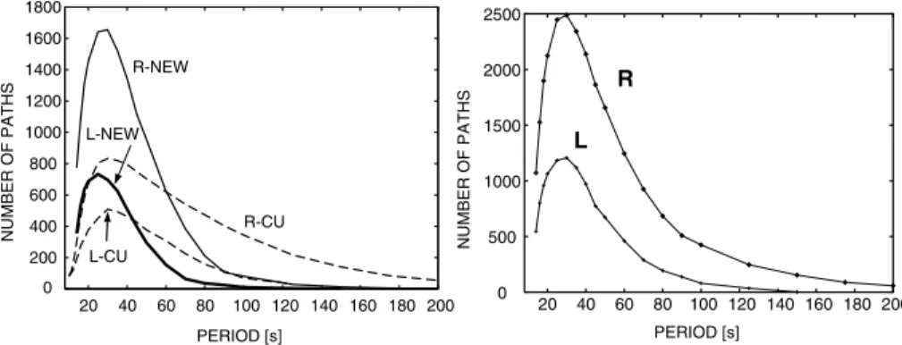
Fig. 2 compares the number of newly analysed Love and Rayleigh

wave measurements with the number in the pre-selected CU data

set. The new data set increases the ray density in the study region

significantly. In particular, for shorter periods the number of rays

crossing the target area is increased by more than 200 per cent for

Rayleigh waves and close to 200 per cent for Love waves. For longer

periods (i.e. T

> 80 s), the percentage of new data significantly drops

because large seismic events, necessary to generate long period

ra-diation, are rare in the study region. Fig. 3 illustrates how the new

data set complements the CU data at periods of 25 and 40 s. Note

that many gaps in the pre-selected CU data set are filled by the new

data. Fig. 4 shows the path densities for the combined data set for

a variety of periods for both Love and Rayleigh waves. Due to the

inhomogeneous distribution of sources and stations the path density

is higher in the western part of the studied region and smoothly

de-grades towards the east. Path density dede-grades as periods rise above

40 s.

(9)

0 200 400 600 800 1000 1200 1400 1600 1800 20 40 60 80 100 120 140 160 180 200 NUMBER OF PATHS PERIOD [s] R-CU L-CU R-NEW L-NEW 0 500 1000 1500 2000 2500 20 40 60 80 100 120 140 160 180 200 PERIOD [s] NUMBER OF PATHS R L

Figure 2. The figure on the left shows the number of observed ray paths, on which Love- (L) and Rayleigh-wave (R) group velocities were measured for the

pre-selected CU-Boulder data set (dashed lines, R-CU and L-CU) and during this new study (solid lines, R-NEW and L-NEW). The figure on the right shows the total number of ray paths in the joint data set used for the inversions in this study.

60˚ W 40˚W 20˚W 0˚ 20˚E

40˚E _60˚E 80˚E

100˚E 120˚ E 140˚E 16 0˚E 60˚ N 80˚N 60˚ W 40˚W 20˚W 0˚ 20˚E

40˚E _60˚E 80˚E

100˚E 120˚ E 140˚E 16 0˚E 60˚N 80˚N 60˚ W 40˚W 20˚W 0˚ 20˚E

40˚E _60˚E 80˚E

100˚E 120˚E 140˚E 160˚E 60˚N 80˚ N 60˚ W 40˚W 20˚W 0˚ 20˚E

40˚E _60˚E 80˚E

100˚E 120˚ E 140˚E 160˚E 60˚N 80˚ N

Rayleigh, 25 s, 2447 paths

Rayleigh, 40 s, 2138 paths

Love, 25 s, 1184 paths

Love, 40 s, 971 paths

Figure 3. Path coverage for Rayleigh and Love waves at 25 and 40 s. Blue paths are the new data from this study and red paths represent data from the

CU-Boulder data set. Note the gaps in the CU data set that are now covered through the new data.

3 2 - D I N V E R S I O N F O R G R O U P

V E L O C I T Y M A P S

A tomographic inversion for 2-D group-velocity maps has been

per-formed for a set of periods between 14 and 90 s following the

proce-dure described by Barmin et al. (2001) and Ritzwoller et al. (2002).

In all cases, we inverted the combined data set of the newly acquired

data and the pre-selected CU-Boulder data. As starting models for

the inversion, the group-velocity maps predicted by the CUB2 global

model (Shapiro & Ritzwoller 2002) were used. This model was

con-structed on 2

◦

× 2

◦

grid using more than 200 000 group velocity

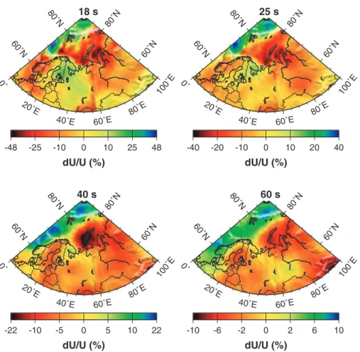
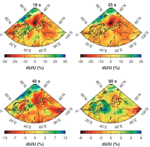
measurements. We present the resulting group-velocity maps for

Love (Fig. 5) and Rayleigh waves (Fig. 7) at four different

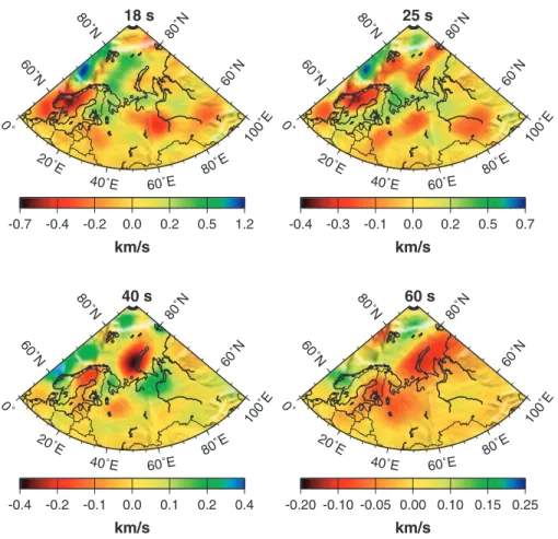
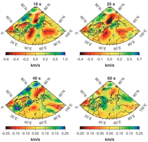
peri-ods: 18, 25, 40 and 60 s. The difference between the new

group-velocity maps and the initial maps is also shown for Love (Fig. 6)

and Rayleigh waves (Fig. 8).

The group-velocity maps show the lateral deviation of the group

velocities from the average velocity in per cent. These deviations

are up to 36 per cent for 16 s Love (Fig. 5) and Rayleigh waves

(Fig. 7). This reflects the strong lateral heterogeneity of the Earth’s

crust in the region, which changes from the mid-oceanic ridge

system in the North Atlantic to thick sedimentary basins in the

(10)

0˚

20˚E

40˚E

_60˚E

80˚E

100˚E

60˚N

80˚N

0˚

20˚E

40˚E

_60˚E

80˚E

100˚E

60˚N

80˚N

0˚

20˚E

40˚E

_60˚E

80˚E

100˚E

60˚N

80˚N

0˚

20˚E

40˚E

_60˚E

80˚E

100˚E

60˚N

80˚N

0˚

20˚E

40˚E

_60˚E

80˚E

100˚E

60˚N

80˚N

0˚

20˚E

40˚E

_60˚E

80˚E

100˚E

60˚N

80˚N

0

10

20

40 80 160 320 640 1280

0˚

20˚E

40˚E

_60˚E

80˚E

100˚E

60˚N

80˚N

0˚

20˚E

40˚E

_60˚E

80˚E

100˚E

60˚N

80˚N

18 s

40 s

25 s

60 s

18 s

40 s

25 s

60 s

LOVE

RAYLEIGH

Path Density

Figure 4. Path density maps for Love (top) and Rayleigh (bottom) waves for different investigated periods. Path density is defined as the number of paths

crossing an equatorial 1◦× 1◦cell.

Barents Sea and old shields with continental crust on mainland

Fennoscandia. Comparison of the resulting and starting maps (Figs 6

and 8) demonstrates significant differences in velocities between the

two sets of maps (up to 1.0–1.2 km s

−1

for short periods and up to

0.25 km s

−1

at period 60 s). This confirms the presence of new

in-formation in the new data set. Table 3 illustrates the improvement

in the data fit achieved by the inversion. We compared the data fit

achieved with selected data to that obtained with a combination of

paths from the CU-B database crossing the studied region and new

data (about 16 000 paths altogether for 40 s period). In the last case,

the rms of the traveltime residuals is twice larger for the paths

in-side the region and the variance reduction for traveltimes residuals

is only

∼10 and ∼9 per cent for group velocities. This could be

expected as the initial model of Shapiro & Ritzwoller (2002) was

built using the CU-B global data set. Including the same data for

a new inversion does not add extra information. This comparison

supports our decision to limit the data set to paths inside the studied

area.

Because the sensitivity kernels for Love waves and Rayleigh

waves are different, Rayleigh waves are sensitive for deeper

struc-tures than Love waves at the same period. Therefore, a joint analysis

of the crustal structure with both Love and Rayleigh waves gives

ad-ditional confirmation for an inverted velocity model. For example,

note that the geographical pattern of group-velocity variations for

Love waves at a period of 25 s (Fig. 5, top right) is similar to the

pattern of group-velocity variations for Rayleigh waves at 18 s

pe-riod (Fig. 7, top left). A similar relation can be found between the

40 s Love and the 25 s Rayleigh waves.

(11)

0˚

20˚E

40˚E _60˚E 80˚E

100˚E 60˚N 60˚N 80˚N 80˚N -48 -25 -10 0 10 25 48 0˚ 20˚E 40˚E 60˚E 80˚ E 100˚E 60˚N 60˚N 80˚N 80˚N -22 -10 -5 0 5 10 22 0˚ 20˚E

40˚E _60˚E 80˚E

100˚E 60˚N 60˚N 80˚N 80˚N -40 -20 -10 0 10 20 40 0˚ 20˚E 40˚E _60˚E 80˚ E 100˚E 60˚N 60˚N 80˚N 80˚N -10 -6 -2 0 2 6 10

18 s

40 s

25 s

60 s

LOVE

dU/U (%)

Figure 5. Results of the 2-D inversion for the group velocities of Love waves with period of 18, 25, 40 and 60 s. The maps present the 2-D distribution of the

inverted group velocities as deviations from the average velocity across the region (in per cent).

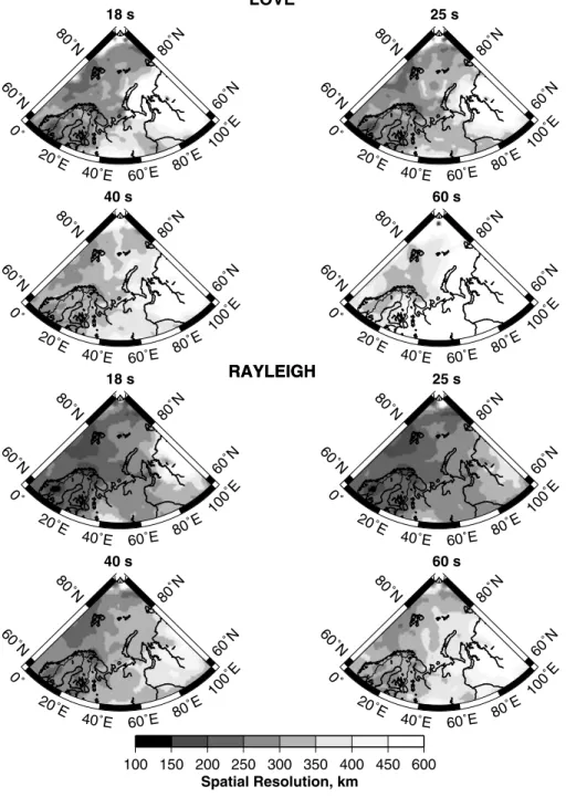
To evaluate the spatial resolution of the estimated group

veloc-ity maps we used the technique described in Barmin et al. (2001).

Fig. 9 illustrates the spatial resolution of the tomographic images for

Rayleigh and Love waves at different periods. The best resolution

(∼200 km) is observed for the Western Barents Sea and

Southeast-ern Barents Shelf. Resolution degrades with increasing period above

40 s. The spatial resolution directly reflects the improvement in path

coverage as shown in Figs 3 and 4.

4 I N V E R S I O N F O R A 3 - D

T O M O G R A P H I C V S M O D E L

The 2-D group-velocity maps at periods up to 90 s derived from

the new data set of Love and Rayleigh wave observations are the

main input for a 3-D inversion for S-wave velocity structure. For

longer periods (up to 200 s for Rayleigh waves and 150 s for Love

waves) the CU-Boulder global group velocity and phase

veloc-ity maps were used as additional input data. Phase velocveloc-ity data

sets were provided by Harvard (Ekstr¨om et al. 1997) and Utrecht

(Trampert & Woodhouse 1995) groups. Due to the small number

of short period surface wave observations, however, the resolution

is limited for details in the structure of the crust, particularly in the

uppermost crust. In addition, shorter period surface waves are much

more influenced by scattering at lateral heterogeneities in the crust.

To improve the inversion with respect to that, we applied the new

crustal model BARENTS50 of the Barents Sea and surrounding

ar-eas, which had been derived in a joint project by the University of

Oslo, NORSAR, and the USGS (Bungum et al. 2005; Ritzmann et al.

2007). This model has detailed information on crustal thickness and

sedimentary basins in the study region with a nominal resolution of

50 × 50 km and helps to constrain the tomographic inversion

partic-ularly in the shallow parts of the resulting inversion. We resampled

the crustal model to a 1

◦

× 1

◦

grid and converted the P-wave

veloc-ities given by Ritzmann et al. (2007) to S-wave velocveloc-ities applying

the P-to-S velocity transformation as used in CRUST2.0 (Bassin

et al. 2000; http://mahi.ucsd.edu/Gabi/rem.dir/crust/crust2.html).

The upper crust of model BARENTS50 with its information on

sedimentary coverage of the greater Barents Sea region was used

as a constraint and not altered during the inversion. The

param-eters of the lower crust and the depth to the Mohoroviˇci´c

dis-continuity were initially taken from model BARENTS50, but

al-lowed to change during the inversion. For the upper mantle part the

CU-Boulder model of Shapiro & Ritzwoller (2002) was used as

the initial model down to a depth of 250 km (see also http://ciei.

colorado.edu/∼nshapiro/MODEL/index.html). Below 300 km, we

applied the Harvard model J362D28 (Antolik et al. 2003) as input.

A smooth transition was used between these two models in the depth

range from 250 to 300 km.

(12)

0˚

20˚E

40˚E _60˚E 80˚E

100˚E 60˚N 60˚N 80˚N 80˚N -0.7 -0.4 -0.2 0.0 0.2 0.5 1.2 0˚ 20˚E 40˚E 60˚E 80˚ E 100˚E 60˚N 60˚N 80˚N 80˚N -0.4 -0.2 -0.1 0.0 0.1 0.2 0.4 0˚ 20˚E

40˚E _60˚E 80˚E

100˚E 60˚N 60˚N 80˚N 80˚N -0.4 -0.3 -0.1 0.0 0.2 0.5 0.7 0˚ 20˚E 40˚E _60˚E 80˚ E 100˚E 60˚N 60˚N 80˚N 80˚N -0.20 -0.10 -0.05 0.00 0.10 0.15 0.25

18 s

40 s

25 s

60 s

LOVE

km/s

Figure 6. Difference between the initial and newly inverted group-velocity maps of Love waves with period of 18, 25, 40 and 60 s (in km s−1).

The new 3-D shear velocity model is constructed using a Monte

Carlo method, which is described in detail by Shapiro & Ritzwoller

(2002). The inversion is performed at each node of a 1

◦

× 1

◦

grid

across the region of the study, and produces an ensemble of

accept-able models that are constrained by a variety of a priori information,

including the initial crustal model. Shapiro & Ritzwoller (2002) fully

describe the set of constraints. The isotropic part of the model in

the mantle is parametrized with B-splines. The model is radially

anisotropic from the Moho to a variable depth that averages about

200 km. We will not discuss the anisotropic properties of the model

but will concentrate only on the isotropic component of shear

veloc-ity V

s

= (V

sv

+ V

sh

)

/2 at all depths. Fig. 10 displays an example

of the inversion at two points: one is in Barents Sea (74

◦

N, 40

◦

E),

and the other in the Western Siberia (70

◦

N, 70

◦

E).

5 D I S C U S S I O N O F T H E 3 - D V E L O C I T Y

M O D E L B A R M O D

The inversion results are presented as deviations in shear wave speed

(in per cent) from the S-wave speed in the 1-D Barey model (Fig. 12,

bottom). Fig. 11 shows several horizontal slices through the model in

the range from 60 to 280 km depth. The horizontal slice for a depth of

45 km is shown in Fig. 12 relative to the 1-D reference model Barey.

The shear velocity cross-sections along several transects across the

studied region are shown in Fig. 13. The positions of these transects

are plotted on the map in Fig. 12. The 3-D model BARMOD reveals

lateral heterogeneities in shear wave speeds in the upper mantle

across the whole region. Of particular interest are the imprints of

first-order changes in the tectonic regimes, such as the mid-Atlantic

ridge, the continent-ocean transition in the Norwegian Sea, and the

thickened crust beneath Novaya Zemlya.

The structure of the lithosphere is naturally very closely related

to its tectonic history. For the Barents Sea region, the evolution

is characterized by repeated cycles of compression and extension

making it a tectonically very complex system. Three stages of

major convergence are known for the region related to the

Tima-nian (600–545 Ma), CaledoTima-nian (440–410 Ma) and Uralian (280–

240 Ma) orogenies (Faleide et al. 2006a,b). Since the last major

tec-tonic activity in the region occurred some 240 Ma, we can assume

that the high-velocity anomaly dipping eastward beneath Novaya

Zemlya (Fig. 13) is not of thermal but of compositional origin. The

timing of the active subduction is uncertain although there is

evi-dence that it occurred as early as at the Timanian stage (Faleide, pers.

comm.). Beneath the East Barents Sea basin, which evolved during

late Permian—early Triassic times by rapid, non-fault-related

sub-sidence (Gudlaugsson et al. 1998), the thickened mantle anomaly

indicates a possible chronological relation of both processes

(thick-ening in the mantle and subsidence in the crust), which in turn both

correlate in time with the Uralian collision. The processes causing

the thickening of the high-velocity anomaly can be both mechanical

(13)

0˚

20˚E

40˚E _60˚E 80˚E

100˚E 60˚N 60˚N 80˚N 80˚N -50 -25 -10 0 10 25 50 0˚ 20˚E 40˚E 60˚E 80˚ E 100˚E 60˚N 60˚N 80˚N 80˚N -13 -7 -3 0 3 7 13 0˚ 20˚E

40˚E _60˚E 80˚E

100˚E 60˚N 60˚N 80˚N 80˚N -35 -20 -10 0 10 20 35 0˚ 20˚E 40˚E _60˚E 80˚ E 100˚E 60˚N 60˚N 80˚N 80˚N -8 -5 -3 0 3 5 8

18 s

40 s

25 s

60 s

RAYLEIGH

dU/U (%)

Figure 7. Results of the 2-D inversion for the group velocities of Rayleigh waves with period of 18, 25, 40 and 60 s. The maps present the 2-D distribution of

the inverted group velocities as deviations from the average velocity (in per cent).

or compositional (phase changes) and the mechanisms linking the

thickening in the upper mantle to basin formation are uncertain. The

location of the Caledonian suture in the Barents Sea region is also

uncertain, but Breivik et al. (2002) showed evidence that it may be

situated in the western Barents Sea, approximately at the western

boundary of the shallow upper mantle high-velocity anomaly. Thus,

this western boundary could be related to lithosphere subducted

during the Caledonian collision. For the Uralian collision, no clear

onset of a subducting slab as an indicator for a suture location can

be identified in the model.

The negative anomalies east and southeast of Svalbard at 140 km

depth correlate nicely in geometry with an area influenced by major

tectonic uplift (Dimakis et al. 1998). To the west, BARMOD clearly

images the imprints of the mid-Atlantic ridge and the extension of

a low-velocity anomaly beneath the continental lithosphere near

the Svalbard Archipelago. In contrast to the high-velocity anomaly

to the east, this low velocity anomaly probably is thermal in

ori-gin, related to break-up of the northeastern Mid-Atlantic during the

Cenozoic. Faleide et al. (2006a) compared BARMOD with

ther-mal modelling across the continent–ocean boundary (Breivik et al.

1999) revealing a clear correlation between the modelled isotherms

and the velocity field.

The velocity variations at 45 km depth, presented in Fig. 12,

re-veal approximately the lateral change in S-wave velocity relevant

for Sn propagation. Engdahl & Schweitzer (2004a,b) described

pro-nounced differences in traveltimes and waveform shapes on

NOR-SAR array recordings of nuclear explosions conducted both at the

northern and at the southern nuclear test side on Novaya Zemlya.

This observation may be explained by multipathing effects due to

the dipping high velocity body.

6 C O N C L U S I O N S

The substantial data set of new surface wave group-velocity

mea-surements combined with existing data from CU-Boulder has

pro-vided the opportunity for constructing a new 3-D shear velocity

model of the crust and upper mantle down to about 250 km depth

beneath the European Arctic. This 3-D Vs model, BARMOD, has

higher spatial and depth resolution than previous models and

clar-ifies or reveals important features of the tectonic setting in the

re-gion: continent-ocean boundary, a dipping slab-like high velocity

zone in the upper mantle and the thermal extension of the

northeast-ern Mid-Atlantic ridge system. The contemporaneous thickening

of the high-velocity body beneath the eastern Barents Sea basin

with crustal subsidence is an intriguing indicator for the presence

of mechanic coupling between crustal and upper-mantle structure,

the details of which are yet poorly understood.

Apart from providing S-wave velocities, BARMOD also

con-tains P-wave velocities and densities which were derived by

(14)

0˚

20˚E

40˚E _60˚E 80˚E

100˚E 60˚N 60˚N 80˚N 80˚N -0.6 -0.4 -0.2 0.0 0.2 0.5 1.0 0˚ 20˚E 40˚E 60˚E 80˚ E 100˚E 60˚N 60˚N 80˚N 80˚N -0.25 -0.15 -0.10 0.00 0.10 0.15 0.25 0˚ 20˚E

40˚E _60˚E 80˚E

100˚E 60˚N 60˚N 80˚N 80˚N -0.4 -0.3 -0.1 0.0 0.2 0.5 0.7 0˚ 20˚E 40˚E _60˚E 80˚ E 100˚E 60˚N 60˚N 80˚N 80˚N -0.20 -0.10 -0.05 0.00 0.10 0.15 0.25

18 s

40 s

25 s

60 s

RAYLEIGH

km/s

Figure 8. Difference between the initial and newly inverted group-velocity maps of Rayleigh waves with period of 18, 25, 40 and 60 s (in km s−1).

Table 3. Statistics of the improvements in data fitting with the newly constructed group-velocity maps: Wave—wave type (Love/Rayleigh);

T—period ;δt0—starting rms of traveltime residuals predicted by the CU-Boulder model;δt—resulting rms of the traveltime residual; St–

variance reduction of traveltime residuals;δU0—starting rms of the group velocity residual;δU—resulting rms of the group-velocity residuals;

SU—variance reduction of the group velocity residuals.

Wave T (s) δt0(s) δt (s) St(per cent) δU0(km s−1) δU (km s−1) SU (per cent)

L 18 42.4 27.8 56.9 0.167 0.109 57.5 L 25 27.0 19.1 49,7 0.110 0.083 43.0 L 40 16.5 12.0 47.5 0.079 0.054 52.0 L 60 14.9 10.3 52.5 0.063 0.050 37.7 R 18 50.8 22.5 80.3 0.172 0.079 79.2 R 25 37.0 15.9 81.5 0.139 0.056 83.6 R 40 17.7 10.1 67.6 0.076 0.040 73.0 R 60 15.8 10.1 58.8 0.066 0.043 57.0

using temperature–velocity relations for mantle material as

de-scribed in Goes et al. (2000) and Shapiro & Ritzwoller (2004).

Among an undefined set of optional applications, this complete

ve-locity and density model for the crust and upper most mantle of

the wider Barents Sea region may be used for refining source

spe-cific traveltime corrections (SSSCs) for regional P and S waves

propagating through the larger Barents Sea region as described

in Ritzwoller et al. (2003). The new 3-D velocity model of the

wider Barents Sea region can be downloaded from the web-page

http://www.norsar.no/seismology/barents3d/.

A C K N O W L E D G M E N T S

For this study, we requested and retrieved broad-band and

long- period data from the Norwegian National Seismic

Net-work (NNSN, University in Bergen), Kola Regional Seismological

Center (KRSC, Apatity), Danmarks og Grønlands Geologiske

Un-dersøgelse (GEUS, Copenhagen), Totalf˚arsvarets

forskningsinsti-tut (FOI, Stockholm), British Geological Service (BGS,

Edin-burgh), the Finish National Seismic Network (FNSN, University

of Helsinki), the international networks (GSN and GEOFON) and

(15)

0˚

20˚E

40˚E

_60˚E

80˚E

100˚E

60˚N

80˚N

0˚

20˚E

40˚E

_60˚E

80˚E

100˚E

60˚N

80˚N

0˚

20˚E

40˚E

_60˚E

80˚E

100˚E

60˚N

80˚N

0˚

20˚E

40˚E

_60˚E

80˚E

100˚E

60˚N

80˚N

0˚

20˚E

40˚E

_60˚E

80˚E

100˚E

60˚N

80˚N

0˚

20˚E

40˚E

_60˚E

80˚E

100˚E

60˚N

80˚N

100 150 200 250 300 350 400 450 600

0˚

20˚E

40˚E

_60˚E

80˚E

100˚E

60˚N

80˚N

0˚

20˚E

40˚E

_60˚E

80˚E

100˚E

60˚N

80˚N

18 s

40 s

25 s

60 s

18 s

40 s

25 s

60 s

LOVE

RAYLEIGH

Spatial Resolution, km

Figure 9. Resolution maps for Love (top) and Rayleigh (bottom) waves for different investigated periods.

data centres IRIS and GEOFON. We gratefully acknowledge the

data made available by these organizations.

We thank Hilmar Bungum for initiating the cooperation of

NORSAR and CU-Boulder, Nils Maercklin for providing us with

a resampled version of the crustal model BARENTS50, Michail

Barmin for creating a transportable version of CU software, and

Jan Inge Faleide for important comments on geotectonical aspects

of this work. A. Levshin is very grateful to the administrations of

the NORSAR and the Department of Geosciences, University of

Oslo, for the opportunity to work for three months at NORSAR. Ch.

Weidle was partly funded by a postdoctoral scholarship of the

Nor-wegian Research Council. We thank the Editor Tim Minshull, Walter

Mooney and an anonymous reviewer for thoughtful and

construc-tive reviews. Most figures have been plotted using GMT (Wessel &

Smith 1995).

This is NORSAR contribution 972.

R E F E R E N C E S

Antolik, M., Gu, Y.J., Dziewonski, A.M. & Ekstr¨om, G., 2003. A new joint model of compressional and shear velocity in the mantle, Geophys. J. Int.,

153, 443–466.

Artyushkov, E.V., 2004. Mechanism of the formation of deep sedimentary basins on continents: The Barents Basin, Doklady RAN, Earth Sciences,

397(5), 595–599.

Artyushkov, E.V., 2005. The formation mechanism of the Barents basin

(16)

Figure 10. Examples of the inversion for acceptable 1-D shear velocity models. (a) and (b) A point in the Barents Sea (74◦N, 40◦E). (c) and (d) A point in Western Siberia (70◦N, 70◦E). (a) and (c) Four dispersion curves obtained from tomographic velocity maps (thick black lines) and the predictions from the ensemble of acceptable models (grey lines) shown in (b) and (d), respectively. (b) and (d) The ensemble of acceptable models where SV and SH velocities are presented with light and dark grey shades, respectively. The corridor of acceptable values is indicated by the solid black lines. The S-wave velocity from the global reference model ak135 (Kennett et al. 1995) is plotted as the dash line.

Barmin, M.P., Ritzwoller, M.H. & Levshin, A.L., 2001. A fast and reliable method for surface wave tomography, Pure appl. Geophys., 158, 1351– 1375.

Bassin, C., Laske, G. & Masters, G., 2000. The current limits of resolution for surface wave tomography in North America, EOS, Trans. Am. geophys.

Un., 81(48), F879, Abstract S12A-03.

Breivik, A.J., Verhoef, J. & Faleide, J.I., 1999. Effect of thermal contrasts on gravity modeling at passive margins: Results from the western Barents Sea, J. geophys. Res., 104, 15 293–15 311.

Breivik, A.J., Mjelde, R., Grogan, P., Shimamura, H., Murai, Y., Nishimura, Y. & Kuwano, A., 2002. A possible Caledonide arm through the Barents Sea imaged by OBS data, Tectonophysics, 355, 67–97.

Bungum, H. & Capon, J., 1974. Coda pattern and multipath propaga-tion of Rayleigh waves at NORSAR, Phys. Earth planet. Int., 9, 111– 127.

Bungum, H., Ritzmann, O., Maercklin, N., Faleide, J.I., Mooney, W.D. & Detweiler, S.T., 2005. Three-dimensional model for the crust and upper mantle in the Barents Sea region, EOS, Trans. Am. geophys. Un., 86, 160–161.

Calcagnile, G. & Panza, G.F., 1978. Crust and upper mantle structure under the Baltic shield and Barents Sea from the dispersion of Rayleigh waves,

Tectonophysics, 47, 59–71.

Chan, W.W. & Mitchell, B.J., 1985. Surface wave dispersion, crustal structure and sediment thickness variations across the Barents shelf, Geophys. J. R.

astr. Soc., 68, 329–344.

Dimakis, P., Braathen, B.I., Faleide, J.I., Elverhøi, A. & Gudlaugsson, S.T., 1998. Cenozoic erosion and the preglacial uplift of the Svalbard-Barents Sea region. Tectonophysics, 300, 311–327.

Ebbing, J., Braitenberg, C. & Skilbrei, J.R., 2005. Basement characterisation by regional isostatic methods in the Barents Sea. NGU Report 2005.074, p. 78.

Egorkin, A.A., Levshin, A.L. & Yakobson, A.N., 1988. Study of the deep structure of the Barents Sea shelf by seismic surface waves, in

Numerical modeling and analysis of geophysical processes, Computa-tional Seismology,Vol. 20, pp. 197–201, ed. Keilis-Borok, V.I., Allerton

Press, NY.

Ekstr¨om, G., Tromp, J. & Larson, E.W.F., 1997. Measurements and global models of surface wave propagation, J. geophys. Res., 102, 8137– 8157.

Engdahl, E.R. & Schweitzer, J., 2004a. Observed and predicted travel times of Pn and P phases recorded at NORSAR from regional events,

Semian-nual Technical Summary, 1 January–30 June 2004, NORSAR Scientific Report,2-2004, 51–56.

Engdahl, E.R. & Schweitzer, J., 2004b. Observed and predicted travel times of Pn and P phases recorded at NORSAR from regional event, EOS, Trans.

Am. geophys. Un., 85(47), Abstract S13B-1050.

Faleide, J.I., Ritzmann, O., Weidle, C. & Levshin, A., 2006a. Geodynam-ical aspects of a new 3-D geophysGeodynam-ical model of the greater Barents Sea region—linking sedimentary basins to the upper mantle structure,

(17)

10˚E 20˚E

30˚E 40˚E 50˚E 60˚E 70˚E