Combined land/sea surface air temperature trends, 1949-1972

COMBINED LAND/SEA SURFACE AIR TEMPERATURE TRENDS, 1949-1972

by

ROBERT STEVEN CHEN

S.B., Massachusetts Institute of Technology (1976)

SUBMITTED TO THE DEPARTMENT OF METEOROLOGY AND PHYSICAL OCEANOGRAPHY IN PARTIAL FULFILLMENT OF THE REQUIREMENTS

FOR THE DEGREE OF

MASTER OF SCIENCE IN

METEOROLOGY AND PHYSICAL OCEANOGRAPHY

at the

MASSACHUSETTS INSTITUTE OF TECHNOLOGY

February 1982

0

Signature of Author___

Department of Meteorology and Physical Oceanography January 14, 1982

Certified by

Reginald E. Newell Thesis Supervisor

Accepted by .- .

Chairman, Department Committee JM? SSACiUTE' VS

COMBINED LAND/SEA SURFACE AIR TEMPERATURE TRENDS, 1949-1972

by

ROBERT STEVEN CHEN

Submitted to the

Department of Meteorology and Physical Oceanography on January 14, 1982 in partial fulfillment of the requirements for the Degree of Master of Science in

Meteorology and Physical Oceanography ABSTRACT

A major deficiency in most previous studies of fluctuations in the earth's climate based on air temperature records has been the dearth of data from oceanic areas and the Southern Hemisphere. This study analyzes a unique collection of ship-based observations of surface air temperature assembled by the U.K. Meteorological Office in parallel with the station-based dataset developed by the National Center for Atmos-pheric Research from the publications World Weather Records and Monthly Climatic Data for the World.

Based on this much more geographically comprehensive database, it is concluded that, during the 24-year period 1949-72, no statistical-ly significant warming or cooling trends were evident in the time series of globally averaged surface air temperature measurements. However, temperature trends did vary latitudinally, with significant cooling in northern extra-tropical latitudes, no trend in equatorial latitudes, and significant but not homogeneous warming in southern extra-tropical latitudes. Time series of air temperatures over land and sea exhibited qualitatively similar behavior over the period 1949-72, indicative of both the comparable quality of the two datasets and the probable lack of significant widespread bias in the land-based measurements due to urban development.

The results of this study underscore the need for dense and geographically comprehensive measurements from both land and ocean areas and from both hemispheres in analyzing the global behavior of the

earth's climate.

Thesis Supervisor; Dr. Reginald E. Newell

ACKNOWLEDGEMENTS

Many different people have assisted me in a variety of ways in the preparation of this thesis. I thank R. Newell for his patience and sup-port; F. Navato, S. Schneider, T. Wigley, R. Madden, R. Chervin, S. Thompson, N. Dalfes, S. Warren, C.K. Folland, and J. Perry for their

advice and comments; K. Huber, S. Ary, J. McNabb, and V. Mills for their administrative support; I. Kole and B. Vaupel for their drafting of figures; and K. Chen for typing an early version of the manuscript. Data were kindly provided by R. Jenne of the National Center for Atmos-pheric Research and by the Director-General of the U.K. Meteorological

Service (Met.0.13). This work was supported by the U.S. Department of Energy under contract DE-ACO2-76EV12195 and by the U.S. National Science Foundation under contract ATM-7718628.AO1. Assistance was also received

from the Department of Meteorology and Physical Oceanography, M.I.T., the Climate Board, National Academy of Sciences, and the International Institute for Applied Systems Analysis. Last but not least, I also thank E. Schmidt, M. Uhlig, D. Knowland, B. and P. Golden, and others for their generous hospitality during the preparation of the thesis and my wife M. Golden for her forbearance, assistance, and moral support.

TABLE OF CONTENTS page ABSTRACT 2 ACKNOWLEDGEMENTS 3 TABLE OF CONTENTS 4 LIST OF TABLES 6 LIST OF FIGURES 7 I. INTRODUCTION 8

II. BRIEF REVIEW OF PAST STUDIES OF THE EARTH'S TEMPERATURE 11 RECORD

-- World Weather Records/Monthly Climatic Data for the World 20

-- Soviet Dataset 22

-- Tropospheric Temperature Data 24

-- Sea Surface Temperature Data 26

-- Comparison of Results 27

-- Summary 33

III. DATA ANALYSIS 36

-- Data Sources 36

-- Analysis Procedure 42

IV. ANNUAL TEMPERATURE TRENDS 52

-- Comparison with Other Studies 52

-- Comparison of Regional Trends 63

-- Comparison of Latitudinal Trends 67

-- Comparison of Land, Sea, and Combined Land/Sea Trends 71

V. MONTHLY TEMPERATURE TRENDS 79

-- Comparison of Land and Sea Data 84

VI. SUMMARY AND CONCLUSIONS 88

APPENDIX A -- Annual Surface Air Temperature Anomalies, 1949-72, 94 for Regions and the Globe.

APPENDIX B -- Monthly Surface Air Temperature Anomalies, January 100 1949 to December 1972, for Regions and the Globe.

5

TABLE OF CONTENTS (continued)

page

ABBREVIATIONS AND SYMBOLS 118

REFERENCES7 120

LIST OF TABLES

page

I. Studies of the Earthla Instrumental Temperature Record of 12 the Past Century Reported in the Formal Literature.

IT. Estimated Temperature Changes between Selected Years. 28

III. Equations Used in This Analysis 44

IV. Correlation Coefficients between Annual Surface Air Tempera- 62 ture Anomalies of This Study and Two Other Studies, 1949-72. V. Correlation Coefficients between Annual Surface Air Tempera- 65

ture Anomalies for Regions, 1949-72.

VI. Selected Statistics for Combined Land/Sea Annual Surface Air 68 Temperature Anomalies for Latitude Bands, 1949-72.

VII. Correlation Coefficients between Land-Only, Sea-Only, and 72 Combined Land/Sea Annual Surface Air Temperature Anomalies

for Regions and the Globe, 1949-72.

VIII. Standard Deviations of Monthly Surface Air Temperature Anom- 81 alies for Regions and the Globe, January 1949 to December

1972.

IX. Correlation and Auto-Correlation Coefficients for Land-Only 82 and Sea-Only Monthly Surface Air Temperature Anomalies for

Regions and the Globe, July 1949 to December 1972.

X. Standard Deviations of Monthly Surface Air Temperature 85 Anomalies for Latitude Bands, January 1949 to December 1972. A-I. Annual Surface Air Temperature Anomalies for the Globe, 94

1949-72.

A-2. Annual Surface Air Temperature Anomalies for the Hemispheres, 95 1949-72.

A-3. Annual Surface Air Temperature Anomalies for the Tropical/ 97 Extra-Tropical Regions, 1949-72.

B-1. Monthly Surface Air Temperature Anomalies for the Globe, 100 January.1949 to December 1972.

B-2. Monthly Surface Air Temperature Anomalies for the Hemi- 103 spheres, January 1949 to December 1972.

B-3. Monthly Surface Air Temperature Anomalies for the Tropical/ 109 Extra-Tropical Regions, January 1949 to December 1972.

LIST OF FIGURES

page

1. Number of Stations with Data in Each 50 x 50 Grid Square: 37

1949,

2. Number of Stations with Data in Each 50 x 50 Grid Square: 38 1972.

3. Average Number of Temperature Observations per Month in Each 40

Oceanic 50 x 50 Grid Square, 1949-72: January.

4. Average Number of Temperature Observations per Month in Each 41 Oceanic 50 x 50 Grid Square, 1949-72: July.

5. Number of Latitude Bands in the Hemispheres and the Globe 49

with Combided Land/Sea Data, 1949-72.

6. Number of 50 x 50 Grid Squares with Combined Land/Sea, Land- 51

Only, or Sea-Only Data, January 1949 to December 1972, for the Globe.

7. Annual Surface Air Temperature Anomalies for the Globe, 1949- 53 72.

8. Annual Surface Air Temperature Anomalies for the Hemispheres, 54 1949-72.

9. Annual Surface Air Temperature Anomalies for the Tropical/ 56

Extra-Tropical Regions, 1949-72.

10. Comparison of Northern-Latitude, Land-Only Annual Surface Air 61 Temperature Anomalies of This Study and Two Other Studies,

1949-72.

11. Slopes of the Multi-Year Trend Lines for Land-Only and Sea- 69 Only Annual Surface Air Temperature Anomalies As a Function

of Latitude Band.

12. Standard Deviations of the Multi-Year Land-Only and Sea-Only 75 Annual Surface Air Temperature Anomalies As a Function of

Latitude Band.

13. Monthly Surface Air Temperature Anomalies for the Globe, 80

January 1949 to December 1972.

14. Comparison of Northern Hemisphere, Land-Only Monthly Surface 83 Air Temperature Anomalies of This Study and Jones et al.

I. INTRODUCTION

Over the past several decades, the behavior of the earth's climate as observed through surface air temperature (SAT) measurements has been the subject of considerable study. In general, most analysts have found long-term global or hemispheric average temperature fluctuations of about 0.5-1.00C during the past century. This has fueled much specu-lation as to the causes and future course of such changes, especially in light of the possibility of human influences on climate (e.g., see SMIC, 1971; U.S. Committee for GARP, 1975; Geophysics Study Committee, 1977; World Meteorological Organization, 1979).

Most previous studies, however, have been based on one of only two distinct sources of data: 1) the World Weather Records (WWR) supple-mented by the monthly publication Monthly Climatic Data for the World (MCDW) and 2) synoptic temperature maps published by the U.S.S.R. Main Geophysical Observatory (GGO) and by the U.S.S.R. Hydrometeorological Center. Unfortunately, even these two sources cannot be considered entirely independent since it is likely that they include data from many of the same stations. Furthermore, both data sources are subject to at

least three major deficiencies. First, the observations are largely from only a limited portion of the globe, namely the Northern Hemi-sphere, which for various reasons has had longer-running and more dense-ly spaced measurements. Second, the data are primaridense-ly from continental areas and sometimes a few islands and ship stations, ignoring vast areas of the oceans. Third, widespread artificial changes could be imbedded in the data due to local temperature trends arising from such influences

as urban development and the movement of stations to airport sites. These deficiencies in existing global temperature datasets are especial-ly critical because they raise serious doubts about whether the trends found in previous studies are indeed representative of the earth's cli-mate as a whole. Geographic shifts in atmospheric circulation patterns, regional variations, or local influences could potentially be misinter-preted as major global climatic changes.

This study seeks to overcome the above deficiencies by the use of extensive ship observations of SAT's collected by the U.K. Meteorologi-cal Office. This dataset provides widespread coverage of the northern and tropical Pacific Ocean, the Atlantic Ocean, and the Indian Ocean for the period 1949-72. Few data exist in polar regions (poleward of

750N and 500S) and in some areas of the Pacific Ocean. Data after 1972

were not available at the time this analysis was begun. Nevertheless, this oceanic dataset provides a global-scale indication of the earth's temperature that is entirely independent from the data used in previous studies. It also increases substantially the total area of the globe with temperature measurements in both the Northern and Southern

Hemi-spheres and should be free from the effect of urban development and thermometer movement.

In the analysis reported here, monthly and annual mean temperature trends for 50-wide latitude belts, regions, and the earth as a whole have been derived from data for land areas, oceanic areas, and combined land/ocean areas over the period 1949-72. These trends provide prelim-inary indications of the degree to which SAT trends for land and ocean

10

correspond on both monthly and interannual time scales. They also form the basis for an independent test of the representativeness of tempera-ture trends derived in other studies.

II. BRIEF REVIEW OF PAST STUDIES OF THE EARTH'S TEMPERATURE RECORD Over twenty-five different studies of the global or hemispheric surface air temperature record have been conducted during the past three decades as listed in Table I. This table lists all such studies reported in the formal literature available to the author arranged by date of first publication. Also included in the table are studies in-volving inferred tropospheric thickness (the geopotential height dif-ference between two surfaces of constant barometric pressure). Publica-tions by the same author or authors are grouped together unless signifi-cant changes were made in the data or analysis. Less than half of the studies include data from the Southern Hemisphere and about ten extend back to the previous century or earlier.

Table I illustrates the wide variety of analysis approaches that have been employed, including many different data-selection procedures, gridding and interpolation methods, and analysis techniques. However, as noted in the introduction, the primary data source in virtually all of the studies is either the WWR and/or MCDW or the GGO maps. One major exception is the study by Starr and Oort (5). They used an independent but rather short-term (1958-63) set of daily radiosonde observations from the M.I.T. General Circulation Data Library (Starr and Oort, 1973; Oort and Rasmusson, 1971) to derive mass-average tempera-tures for the entire troposphere (1000 to 50 mb). Several other

For a detailed review of early studies of temperature at individual stations or in limited areas, see Veryard (1963).

Table I. Studies of the Earth's Instrumental Temperature Record of the Formal Literature. Study/Reference 1. Willett (1950) 2. Callendar (1961a) 3. Mitchell (1961, 1963, 1970) .4. Budyko (1969, 1977); Spirina (1969, 1970)

5. Starr & Oort (1973) Type of Temperature Series 5-yr deviations from 1935-40 stn. means deviations from 1901-30 stn. means 5-yr deviations from 1880-84 stn. means deviations from long-term stn. means mass-average val-ues & nonseasonal deviations for surface-75 mb Period and Time Unit 1845-1940; pentads (annu-al & winter) 1870-1950; annual 1870-1960 (later to 1967); pentads

(annual & win-ter) 1881-1960 (later to 1967); annual Latitudinal Coverage and Number of Stations 700S-800N; 183 stns. 600S-730N; over 400 stns. 600S-800N; 118-179 stns. 200N-800N; stns. unknown 1958-63; annu- 00-900N; al & monthly "300-600 stns.

Past Century Reported in the

Grid and Interpolation Method 100 x 10lO** 1 stn./ grid pt. latitude bands S600S-250S, 25 S-250N, 250 N-600N, 600N-73 ON); avg. of stns. in band 100 x 100**; 1 stn./ grid pt. 50 x 100*lO map analysis 50 x 50** objective analysis Data Sources Notes WWR (plus 4 other stns.) WWR (plus misc. stns.) WWR, Scherhag (1965, 1966, 1967) GGO MIT

A) 4 4 Table I (continued) Study/Reference 6. Reitan (1974) (update of 1 & 3) 7. Dronia (1974) 8. Angell & Korshover (1975) 9. Yamamoto et al. (1975, 1978) 10. Brinkmann (1976) (update of 1, 3, & 5)

11. van Loon &

Williams (1976a, b), Williams & van Loon (1976) Type of Temperature Series 5-yr deviations from 1955-59 stn. means deviations from 1949-73 means for 1000-500 mb deviations from 1958-73 stn. means for 700-300 mb Period and Time Unit Latitudinal Coverage and Number of Stations 1955-68; 00-800N;

pentads (annu-"200 stns. &

al & winter) misc. SST data)

1949-73; annual 1958-73; annual & sonal sea-deviations from 1951-72; 1951-72 stn. means monthly 2 50-9 0 0N; stns. unknown 750S-750N; 45 stns. 2 0oS- 8 50N; 343 stns.

5-yr deviations 1969-73; pen- 00-80oN;

from 1965-68 stn. tads (annual & &200 stns. &

means seasonal) misc. SST data)

means of stn. re- 1900-72;

gression coeffi- seasonal

cients for over-lapping 15-yr periods 150N-800N; &300 stns. Grid and Interpolation Method 100-wide lati-tude bands; avg. of stns. in band 50 x 100** map analysis latitude bands centered at 75 OS 450S 200S, 20 N, 45 N, 75 ON; avg. of stns. in band 50 x 50** ; cubic spline 100-wide lati-tude bands; avg. of stns. in band 50 x 50** map analysis Data Sources Notes WWR, MCDW, d misc. SST maps FRG MCDW WWR, MCDW MCDW, misc. g SST maps WWR

4*p 40 e0 Table I (continued) Study/Reference Type of Temperature Series

12. Borzenkova et al. deviations from

(1976) long-term stn.

means (corrected)

13. Damon and Kunen

(1976)

means of stn. SAT observations for solar cycles & pentads Period and Time Unit 1881-1975; monthly 1943-74; solar cycles 1955-74; pen-tads Latitudinal Coverage and Number of Stations 17.50N-87.50N; stns. unknown 900S-00; 67 stns. Grid and Interpolation Method 5° x 100**; map analysis latitude bands

S90oS-450S,

15. van Loon &

Williams (1977)

16. Kukla et al.

(1977) Tupdate of 7, 8, & 9)

same as 11, plus 1949-72; win- 150N-800N;

700 mb temperature ter 300 stns.

1956-73; win- 90°S-400S;

ter 24 stns.

same as 7, 8, & 9 7: 1949-76 same as 7, 8;

(except base 8: 1958-76 NH 9: 300S-90 N; period of 1951- 1958-75 SH 350 stns. 75 for 9) 9: 1951-75 ann. 1965-75 seas. 50 x 50** map analysis same as 7, 8, & 9 WWR, NMC k same as e, 7, 8, & 9 f

Table I (continued) Study/Reference 17. Harley (1978) 18. Angell & Korshover (1978a) 19. Barnett (1978) 20. Yamamoto & Hoshiai (1979) 21. Harley (1980) 22. Yamamoto & Hoshiai (1980) 23. Vinnikov et al. (1980) Type of Temperature Series Period and Time Unit deviations from 1949-76;

1959-65 and 1965- 12-mo. moving

75 means for 1000- avgs.

500 mb

deviations from 1958-77;

1958-77 stn. means seasonal for surface &

sur-face-100 mb

deviations from 1950-77;

1950-77 stn. means annual & win-ter

deviations from 1951-77;

1951-75 stn. means monthly

5-yr deviations 1949-78;

between successive pentads pentads for 1000-500 mb deviations from 1876-1975; 1931-60 stn. means seasonal deviations from 1881-1978; long-term stn. annual means (recorrected) Latitudinal Coverage and Number of Stations 250N-850N; stns. unknown 900S-900N; 63 stns. 150N-650N; 424 land & ocean stns. 250N-900N; 370 stns. 250N-900N (383 grid pts.); stns. unknown 250N-900N; 367 stns. 17.50N-87.50N; stns. unknown Grid and Interpolation Method 50 x 50** map analysis same as 14 100 x 200** avg. of stns. in grid sq. 100 x-30* (450 at 800N); optimum inter-polation 50 x 10**; map analysis same as 20 50 x 10** map analysis Data Sources FRG, UK, CMC MCDW MCDW, TDF11 Notes WWR, MCDW, ATW FRG, UK, CMC same as 20 o GGO

40 40

Table I (continued)

Study/Reference

24. Boer & Higuchi

(1980, 1981) 25. Navato et al. (1981) 26. Hansen et al. (1981) 27. Jones et al. (1981) Type of Temperature Series mean thickness for 1000-500 mb deviations from 1958-78 stn. means for 700-300 mb deviations from long-term stn. means deviations from 1946-60 stn. means Period and Time Unit Latitudinal Coverage and Number of Stations 1949-75; annu- 250N-900N;

al & seasonal stns. unknown 1958-78; monthly 1880-1979; annual 900S-82.50N; 34 stns. 900S-900N; "several hun-dred" stns. 1881-1980; 00-900N; monthly, sea- 300-1300 stns. sonal, &

annu-al Grid and Interpolation Method 50 x 50 * * map analysis latitude bands (900S-200S, 20 S-200 N, 20oN-900N); avg. of stns. in band 80 equal-area boxes; succes-sive avg. of stns. in box Data Sources Notes MCDW WWR, MCDW 50 x 100**; WWR, MCDW, t inverse- misc. stn.

distance weight data algorithm

for abbreviations, see ABBREVIATIONS AND SYMBOLS.

** latitude by longitude.

40 4#

Table I (continued)

Notes

a See also, Landsberg and Mitchell (1961), reply by Callendar (1961b), and Veryard (1963).

b According to Borzenkova et al. (1976), deviations for 1881-1940 were computed relative to the base period 1881-1935 for most stations and 1881-1940 for the remainder; and for 1941-60 relative to

the base period 1881-1960.

c Observations taken at 0000 GMT. Interpolation to grid points using Conditional Relaxation Analysis

Method. See Oort and Rasmusson (1971) for further details; also see Hawson (1974) and reply by

Starr and Oort (1974).

d Used selected SST data as surrogate for SAT's in the Pacific Ocean. Data from Eber et al. (1968), the Japan Meteorological Agency, and the U.S. Bureau of Fisheries.

e Notes possible artificial cooling trend due to gradually improving radiosondes in the U.S.S.R. f Observations normally taken at 1200 GMT. Stations selected at mean latitudes as given.

g As noted in d, but additional data from Fishing Information (National Marine Fisheries Service). h Linear regression coefficients were calculated for station data for overlapping 15-year periods

at 5-year periods. Coefficients were then plotted and zonally averaged.

i Basic data as in note b, plus deviations for 1961-69 were computed relative to the base period 1881-1935 and for 1970-75 relative to 1931-60. Corrections derived from anomaly maps (see

Vinnikov et al., 1980, for more details). See also, Budyko and Vinnikov (1976), Rubinshtein

(1977), and Vinnikov (1977).

j

qk) '.

Table I (continued)

Notes (continued)

k Linear regression coefficients were calculated for station and 700 mb grid-point data for the

entire 24-year series and then plotted and zonally averaged. 700 mb data are from daily maps

prepared by the U.S. National Meteorological Center.

1 Data for 1949-65 are from the Deutscher Wetterdienst via the U.K. Meteorological Office; for

1965-71 from the U.K. Meteorological Office; and for 1971-76(78) from the Canadian

Meteoro-logical Centre. Data from the Pacific Ocean is missing until 1966. Observations taken at 0300 GMT until 1957 and 0000 GMT thereafter.

m See update in Angell and Korshover (1978b) and data for 100-30 mb (42 stations).

n. Also used empirical orthogonal functions to analyze annual average temperature anomalies. Data as in note g. Ocean stations chosen on a 500-800 km grid.

o Optimum interpolation assumes zero deviation when no data exists at a grid point, causing underestimation of anomalies in data-sparse regions.

p Basic data and procedures as in note i, except a more complex system of corrections. Anomaly values were reread from maps with a slightly different grid (not specified).

q Basic data from the U.K. Meteorological Office. Observations taken twice daily. Pacific Ocean

data south of 550N missing before 1965. Cf. Harley, note 1.

r Used method of Angell and Korshover (1975), with more limited station network and additional data checking.

s Used digitized version of WWR and MCDW data prepared at the National Center for Atmospheric Research (Jenne, 1975) with additional recent data from MCDW.

Table I (continued)

Notes (continued)

t As in r, plus additional data from CLIMAT network, Danish and Icelandic Meteorological Services, and miscellaneous Norwegian and Soviet sources. See also, Jones and Wigley (1980a,b,c,d) and Wigley and Jones (1981).

studies also derive tropospheric temperature changes, but do so indi-rectly from geopotential height data (7, 8, 14, 17, 21, 24, and 25). In some instances, sea surface temperature (SST) data from various sources were used as a surrogate for SAT measurements over the oceans (6, 10, and 19), but the degree to which these climatological parameters correspond is a major uncertainty. In many studies (e.g., 1, 2, 3, 20, 22, and 27), additional station data were also obtained from miscellane-ous sources such as national meteorological services. Each of the prin-cipal data sources above, and the analyses that have been applied to them, warrant brief discussion.

World Weather Records/Monthly Climatic Data for the World

The World Weather Records contain monthly average temperature data from over 2500 individual stations around the world, with a few records that extend back as far as the early 1800's. Until 1940 they were published by the Smithsonian Institution (Clayton and Clayton, 1927, 1934, 1947) and from 1941-60 by the U.S. Department of Commerce, U.S. Weather Bureau (1959, 1965-68). More recently, global climatological

data (including radiosonde observations) have been disseminated in Monthly Climatic Data for the World (U.S. Department of Commerce, 1961-present), a monthly publication produced under the auspices of the World Meteorological Organization. The dataset is now available in

computer-readable form from both the National Climatic Center and the National Center for Atmospheric Research (Jenne, 1975).

Unfortunately, data coverage in the WWR and MCDW is neither geo-graphically complete nor continuous in time. As Figures 1 and 2 (next

chapter) illustrate for the period of interest in this study (1949-72), measurement stations are primarily located in continental areas, with

some island sites and a few ship stations. Although the geographic coverage generally increases between Figures 1 and 2, the number of stations does decrease in a few squares, indicative of the transience of station records in the dataset. At least part of the lack of con-tinuity may have arisen from the transition between the WWR and MCDW. Jones et al. (1981), for example, report a sharp drop in data coverage after 1960 due to the omission in MCDW of station records primarily from

the tropics that had been reported in the WWR.

Several different methods have been used to compensate for irregu-lar station spacing to avoid giving undue weight to data-rich regions. The simplest approach (used in studies 1, 3, 6, 8, 10, 14, 16, 18, and

25) is to develop a reasonably regular but coarse grid by carefully selecting one station to represent an area or grid point. Alternative-ly, data from all stations within the same grid square can be averaged together, using somewhat complicated algorithms or weighting schemes if desired (e.g., studies 2, 19, 26, and 27). A third approach is to inter-polate data between stations to regular grid points using some interpola-tion method such as cubic splines or optimum interpolainterpola-tion (studies 5, 9, 16, 20, and 22). A major disadvantage of optimum interpolation is that grid points with no data are implicitly assigned an anomaly value of zero, leading to underestimation of the temperature trend (Yamamoto and Hoshiai, 1979, 1980).

The lack of continuous data at many stations raises the possibility of introducing false trends due to the addition or subtraction of sta-tion records. One method to avoid this problem, used by Damon and Kunen (13), is simply to select stations with records of equal length, employing some form of interpolation to fill in any missing data. How-ever, most of the studies in Table I extract trend information by calcu-lating temperature deviations or "anomalies" from the mean value over some base period at each station or grid point. The use of temperature anomalies has the added advantages of eliminating the need to adjust station temperature observations to the same altitude and of permitting the removal of the mean seasonal cycle from monthly or seasonal data. Alternatively, van Loon and Williams (11, 15) estimate the linear re-gression coefficients of station temperature data for successive but overlapping 15-year periods (at 5-year intervals). These coefficients were then interpolated to grid points by subjective map analysis and averaged zonally.

Soviet Dataset

The data and procedures used by Soviet analysts are reviewed in some detail by Jones et al. (1981). In brief, the Soviet studies (4, 12, and 23) essentially rely on monthly mean temperature maps for the Northern Hemisphere over the period 1881-1935, prepared by a group from the GGO (Sokhrina et al., 1959). These in turn formed the principal basis for maps of temperature anomalies over the period 1881-1960

(Sharov, 1960-67). Maps of anomalies for 1961-75 were prepared by the U.S.S.R. Hydrometeorological Center (Gidromettsentr, 1961-78). Anomaly

values were read off from the maps at regular grid points and used to compute zonal means.

The Soviet maps unquestionably include data from stations common to the WWR and MCDW, but the extent of overlap is not clear at this time. Information on the stations used to generate the original temper-ature and anomaly maps is not available, nor are the procedures for treating data-sparse areas and irregular station observations docu-mented. As with the WWR and MCDW, it is clear that coverage of oceanic areas is poor. Moreover, the latitudinal coverage of the Soviet data

(17.50N - 87.50N) is comparatively limited.

As indicated in detail in notes b and i of Table I, different base periods were used to compute the anomalies for different portions of the Soviet data. Borzenkova et al. (1976) developed a simple correction procedure to make anomalies more homogeneous without referring back to the original temperature data. Vinnikov et al. (1980) reread the anoma-ly values from the maps for the period 1891-1978 and recomputed the time series. They employed a slightly modified version of the correction procedure of Borzenkova et al. for continental grid points and a differ-ent procedure based on archives of air temperature normals for the re-maining grid points. As pointed out by Jones et al. (1981), the uncor-rected series of Budyko (4) and Vinnikov et al. (.23) do differ notice-ably, by roughly a tenth of a OC generally, but are still highly cor-related (r = 0.98).

Tropospheric Temperature Data

Starr and Oort (5) took advantage of a comprehensive data archive at the Massachusetts Institute of Technology (MIT), compiled for a

study of the atmospheric general circulation (see Oort and Rasmusson, 1971). This archive includes radiosonde observations made once daily at approximately 0000 GMT at nearly 600 stations in the Northern Hemisphere over the period 1958-63. Available daily data at the 1000, 950, 900, 850, 700, 500, 400, 300, 200, 100, and 50 mb levels were interpolated to regular grid points by an objective analysis algorithm and then averaged

into monthly means and into mass-average values for the troposphere. The mass-average values thus incorporate considerably more temperature

information than contained in just surface temperature measurements. However, the short period of this record limits its usefulness as an

independent test of the other SAT datasets.

Various studies by Dronia (7, 16), Angell and Korshover (8, 14, 16, and 18), Harley (17, 21), Boer and Higuchi (24), and Navato et al. (25) extend the tropospheric time series by utilizing data on geopotential height differences. Dronia (1974) used monthly pressure charts prepared by the Deutscher Wetterdienst (FRG) as the basis for estimating free-air

temperatures below 500 mb (roughly 5.5 km) at regular grid points.

Harley (1978, 1980) performed a similar analysis with data from the U.K. Meteorological Office (which included some FRG data) and the Canadian Meteorological Centre (CMC). Boer and Higuchi (1980, 1981) essentially repeated Harley's analysis but with twice-daily data from the U.K. Mete-orological Office. Angell and Korshover (1975, 1977, 1978a), in

contrast, chose a sparse grid of 45-63 radiosonde stations reported in MCDW and derived time series for both free-air and surface temperature trends. Navato et al. (1981), in following the method of Angell and Korshover (1975), used even fewer stations than the latter, but more carefully scrutinized the observations and produced a monthly time

series. In general, the above studies appear to have results consistent with each other and with Starr and Oort (5), although some differences

in absolute values appear due to the different data bases and proce-dures.

The utility of the tropospheric temperature trends as an independ-ent check of the surface air temperature record is an unresolved issue. Tropospheric and surface air temperatures are controlled by different but interactive radiative and dynamic processes. Changes in atmospheric

circulation patterns, for example, might involve large changes in sur-face air temperature with minimal changes in upper air temperatures (van Loon and Williams, 1977). In addition, radiosonde observations suffer from many of the same difficulties as surface measurements, in-cluding very scattered, land-based stations and possible measurement problems (e.g., see van Loon and Williams, 1976a; Hawson, 1974; Starr and Oort, 1974). Thus, although agreement between surface and tropo-spheric air temperature trends would be an encouraging sign, disagree-ment between;:them could arise for a variety of reasons that might be difficult to separate.

For example, see Angell and Korshover (1975), table I, and Harley (1978), table 2. Also, compare bottom two curves of Navato et al. (1981), figure 1, with Angell and Korshover (1975), figure 3.

Sea Surface Temperature Data

Studies by Reitan (6), Brinkmann (10), and Barnett (19) use SST data to increase the sampling of temperature in oceanic areas of the Northern Hemisphere. Reitan (1974) obtained SST data for the Pacific Ocean over the period 1955-68 from maps prepared by Eber et al. (1968), the Japan Meteorological Agency, and the U.S. Bureau of Fisheries (c.f., Newell and Hsiung, 1979). In his update of Reitan, Brinkmann (1976) added SST data for 1969-73 in both the Atlantic and Pacific Oceans. However, neither of these authors supply any indication of the geo-graphic extent or treatment of these data in their published materials. Barnett (1978) combined extensive SST data from the "Marine Deck"

(TDF11) maintained by the National Climatic Center with continental data from MCDW. His dataset includes almost as many oceanic stations as continental stations. He first calculated anomaly values for both land and sea data and then averaged values within each 100 x 200 square. He also analyzed the spatial and temporal patterns of temperature variance

by the use of empirical orthogonal functions, obtaining a coherent first

eigenvector that correlates well (r = 0.66) with the hemispheric mean curve derived in his study.

All of these studies assume that SST's and SAT's are reasonably

well correlated, at least on seasonal and annual time scales. This assumption is supported by the analyses of Newell and Weare (1976), Navato et al. (1981), Newell and Chiu (1981), and others. However, the latter studies also raise the possibility of connections between extra-tropical SAT's and extra-tropical SST's and of lagged relationships between

SAT's and SST's. If borne out, these preliminary findings would greatly complicate the interpretation of temperature trends based on both SST's and SAT's. Moreover, SST data have their own potentially serious prob-lems with respect to measurement biases and procedural changes (e.g., "intake" versus "bucket" temperature measurements; Barnett, personal communication, 1981). Further examination of this approach will clearly be necessary.

Comparison of Results

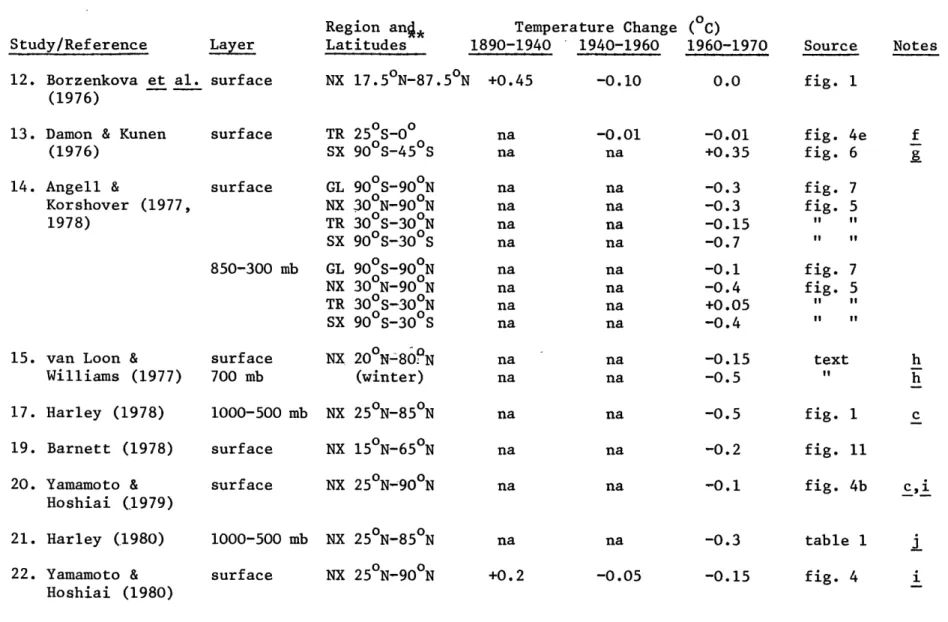
Despite the often substantial differences in ldata selection and analysis procedures described in the previous sections, all of the studies in Table I appear to have reasonably comparable results. Table II provides an admittedly simplistic comparison of the trends. Studies in this table are arranged in the same order as Table I. Temperature changes were estimated between single years (except as noted) to provide a rough indication of the sign and approximate magnitude of the trends. The years 1890, 1940, 1960, and 1970 were arbitrarily chosen to span periods of interest and ensure maximum possible overlap between studies.

For northern latitudes, the studies that extend back into the pre-vious century (studies 1, 2, 3, 4, 12, 22, 23, 26, and 27) report a general warming of between 0.2°C and 0.7°C from 1880 to 1940. The low value by Yamamoto and Hoshiai (22) may have arisen from their use of optimum interpolation. Greater warming is apparent at higher northern

latitudes and in winter in those studies with regional and seasonal breakdowns (e.g., see Mitchell, 1963, Table 5; Vinnikov et al., 1980, figure 1; and Wigley and Jones, 1980 a,d). From 1940 to 1960, the

Table II. Estimated Temperature Changes between Selected Years.

Study/Reference

1. Willett (1950)

Layer surface 2. Callendar (1961a) surface

3. Mitchell (1961, 1963, 1970) 4. Budyko (1969) 6. Reitan (1974) 7. Dronia (1974) 8. Angell & Korshover (1975) 9. Yamamoto et al. (from Kukla et al., 1976) 10. Brinkmann (1976) 11. Williams & van

Loon (1976) surface surface surface 1000-500 mb 700-300 mb surface surface surface Region and Latitudes** GL 70oS-80 0N GL 60oS-600N NX 250N-600N TR 250S-250N SX 600S 250S GL 600S-800N NH 00-800N TR 300S-300N SH 60oS-00 NX 200N-800N NH 00-80 0N NX 350N-900N NH 00-75 0N TR 20oS-20oN SH 750S-00 NH 00-900N TR 200S-0 NH 00-800N NX 150N-800N

1890-Temperature Change (oC)

-1940 1940-1960 1960 +0.5 +0.41 +0.44 +0.49 +0.33 +0.4 +0.6 +0.4 +0.4 +0.45 na -1970 Source Notes fig. 1 na na na na na na -0.25 na na -0.15 -0.2 na na na -0.55 -0.5 -0.3 -0.2 -0.1 0.0 -0.07 -0.26 Appendix If fig. fig. fig. fig. 1(1961) 1(1970) 4(1961) 1(1970) fig. 1 fig. 1 fig. 3 fig. It II fig. 3/101 c fig. 3/104 c table 1 d table 1

* 4.

Table II (continued)

Study/Reference Layer

Region an* Latitudes

Temperature Change (OC)

1890-1940 1940-1960 1960-1970 Source Notes

12. Borzenkova et al. surface

(1976)

13. Damon & Kunen

(1976)

14. Angell &

Korshover (1977, 1978)

15. van Loon &

Williams (1977) 17. Harley (1978) 19. Barnett (1978) 20. Yamamoto & Hoshiai (1979) 21. Harley (1980) 22. Yamamoto & Hoshiai (1980) surface surface 850-300 mb surface 700 mb 1000-500 mb surface surface 1000-500 mb surface NX 17.5 0N-87.50N TR 250S-0 0 SX 900S-450S GL 900S-900N NX 300N-900N TR 30 S-300N SX 90 S-300S GL 900S-900N NX 300N-900N TR 300S-30 0N SX 900S-300S NX 200N-80"N (winter) NX 250N-850N NX 150N-650N NX 250N-900N NX 250N-850N NX 250N-900N +0.45 -0.10 -0.01 na na na na na na na na na na na 0.0 -0.01 +0.35 -0.3 -0.3 -0.15 -0.7 -0.1 -0.4 +0.05 -0.4 -0.15 -0.5 -0.5 -0.2 -0.1 -0.3 +0.2 -0.05 -0.15 fig. 1 fig. 4e fig. 6 fig. fig. If if fig. 7 fig. 5 It II It II text It fig. 1 fig. 11 fig. 4b c,i table 1 fig. 4

Table II (continued)

Study/Reference

23. Vinnikov et al.

(1980)

24. Boer & Higuchi

(1980) 25. Navato et al. (1981) 26. Hansen et al. (1981) 27. Jones et al. (1981) Layer surface 1000-500 mb 700-300 mb surface surface Region anj, Latitudes NX 17.50N-87.50N NX 250N-900N NX 200N-82.50N TR 200S-20 N SX 900S-200S GL 90°S-90 0N NX 23.60N-900N TR 23.6OS-23.60N SX 900S-23.60 S NH 00-900N

Temperature Change (oC)

1890-1940 1940-1960 1960-1970 +0.47 -0.10 -0.07 -0.5 na na +0.4 +0.7 +0.3 +0.2 +0.48 -0.05 -0.1 0.0 -0.1 -0.04 -0.08 +0.01 -0.08 -0.05 -0.4 0.0 +0.25 -0.21 Source Notes table 2 fig. 1 pers. comm.l 1 " 1 " "

T

Unsmoothed annual values for 1890, 1940, 1960, and 1970 obtained except as noted from tables in the

cited reference if available or by visual inspection of figures (to 0.050C if possible). Study

numbers correspond to Table I. Only studies with published data are included.

Abbreviations as given in ABBREVIATIONS AND SYMBOLS; however, the boundary between the tropics and

Table II (continued)

Notes

a Temperature change between pentads 1890-94 and 1930-34.

b Temperature change estimated from curve of inter-pentadal mean temperatures. c Annual values estimated visually from monthly data.

d Temperature change between periods 1960-64 and 1970-73. e Temperature change between 1942 and 1972.

f Temperature change between solar cycles 23 (mid-1943 to mid-1953) and 24 (mid-1953 to mid-1963) for 1940-60 value and between solar cycles 24 and 25 (mid-1963 to mid-1974) for 1960-70 value. g Temperature change between pentads 1960-64 and 1970-74.

h Winter temperature change estimated by assuming a linear decrease over the 24-yr. period 1949-72. i Temperature change may be underestimated due to use of optimum interpolation.

j Temperature change between pentads 1959-63 and 1969-73.

k Assumed 20-meter change equals 1 C, as in Harley (1978).

Northern Hemisphere trend reverses, with a general cooling of 0.04-0.250C. This cooling appears to end in the mid-1960's, and in many of the studies a warming becomes noticeable by about 1970. For example, in figure 1 of Borzenkova et al. (1976), the northern extra-tropical

temperature drops by almost 0.40C from 1960-65, but by 1970 has regained the 1960 level. Notably, the cooling in the northern extra-tropical troposphere is generally larger than the surface cooling (see van Loon and Williams, 1977).

The general agreement among the studies in Table II regarding the temperature behavior of the Northern Hemisphere climate is supported by the analysis of Jones et al. (1981). They found high, significant cor-relations (with almost all coefficients greater than 0.70) among their Northern Hemisphere mean annual SAT trends and those of Budyko (1969),

Reitan (1974), Yamamoto et al. (1975), Barnett (1978), Angell and

Korshover (1978a), and Asakura over periods for which these time series overlap. They note, however, that such high correlations should be expected because of the common source of raw station data.

Only a few studies present trends for the tropics. From 1890-1940, three studies (2, 3, and 26) report an increase of 0.3-0.490C. Negligi-ble change is apparent over the period 1940-60 (13, 26). However, exam-ination of figure 3 of Hansen et al. (1981) shows that temperatures did decrease by about 0.050C during this period, but regained the 1940 level

As reported in Angell and Korshover (1977) and U.S. Committee for GARP (1975). Otherwise, not formally published.

by 1960. A similar cycle occurs from 1960-70, leading to the low values

for this period given in studies 8, 9, 13, 14, 25, and 26.

In southern latitudes, a warming of 0.2-0.40C is apparent from 1890-1940 in studies 2, 3, and 26. From 1940-60, Hansen et al. (1981) indicate fluctuations of about 0.20C, yielding a small net cooling of just 0.10C. During the decade 1960-70, a disagreement as to the sign of the trend emerges among the different studies. Damon and Kunen

(1976) and Hansen et al. (as well as this study) show a substantial

surface temperature increase of a few tenths of a OC, which appears to continue into the early 1970's. In contrast, Angell and Korshover

(1977) report a 0.70C surface temperature decrease, and Angell and

Korshover (1975, 1977) and Navato et al. (1981) a 0.08-0.40C tropo-spheric temperature decrease. The latter studies do indicate that the trend reverses to a warming in the early 1970's. The origin of this discrepancy, especially between the surface temperature curves of Angell and Korshover (1977; see also, 1978a) and those of Damon and

Kunen (1976) and Hansen et al. (1981), is discussed further in the next chapter.

Summary

As evidenced by Table II, all of the previous studies of the earth's air temperature record do appear to agree qualitatively as to the general temperature behavior of the climate over the past century, with only one noticeable exception during 1960-70 in the Southern

Hemisphere. Estimates of the magnitude of the trends of course differ somewhat, as would be expected given the differing data sources and analysis procedures and the simple point estimates of trends used here.

It is important to note, however, that the general agreement among the studies in Table II could be the result of the large amount of data that they probably have in common. Most studies of the surface air temperature have drawn on the station measurements recorded in the WWR and MCDW, and several of the studies of tropospheric temperature use

similar datasets. The latter, moreover, involve a very sparse network of upper-air observing stations. The sea surface temperature is an in-dependent, densely measured climatological parameter, but its utility as a surrogate for air temperature is uncertain at present. SST data are also subject to other problems regarding possible false trends and mea-surement biases.

The past reliance on land-based station measurements of air tempera-ture (or geopotential height) primarily from the Northern Hemisphere could lead to significant problems in understanding properly the

behav-ior of the climate in both the past and the future. For example, as demonstrated by Parker (_1981), if the air temperature over the land is greater than that over the sea, measurements restricted to land-based

stations could greatly overestimate zonal mean temperature variations. Shifts in the mean position of troughs and ridges in zonal temperature patterns could generate apparent trends in land-based data that would not accurately represent the actual behavior of the zone or region. Similarly, excessive reliance on Northern Hemisphere data could be

deceptive given that observations from only one region may not be repre-sentative of the earth's overall temperature behavior. Internal redis-tributions of heat within the climate system might, for example, result

in warming in one region compensated by cooling in another. Finally, widespread measurements in land-based temperature measurements are pos-sible due to such local but pervasive influences as urban development and its associated "heat island" effect and the movement of thermometers to airport sites (e.g., see Mitchell, 1953).

To help avoid the kinds of problems listed above, it is clear that some independent indicator of the earth's temperature behavior is needed. This thesis, in examining ship observations of air temperatures over the oceans, is an initial attempt to meet this need.

III. DATA ANALYSIS

In this thesis, use was made of two independent sets of SAT obser-vations over the period 1949-72. Land data in the form of monthly

averages were extracted from the World Monthly Surface Station Climatol-ogy maintained by the National Center for Atmospheric Research (NCAR) and based on the WWR and MCDW. Monthly sea data were obtained from the U.K. Meteorological Office, which collected ship observations of SAT's and averaged them into monthly values for 10 x 10 grid squares. As described in this chapter, these two datasets were processed in a

simi-lar fashion to provide the highest practical compatibility. Efforts were also made to ensure comparability with the results of other studies.

Data Sources

As noted above, land observations of SAT's were obtained from a magnetic tape prepared at NCAR from the WWR and MCDW (Jenne, 1975; see also, Spangler and Jenne, 1977). Over the period 1951-70, this dataset contains temperature records from approximately 1700 stations with an average of about 10 months of data per year per station (see Jenne,

1975, Table 10-1). Monthly temperature means are recorded to the nearest 0.10C along with the numbers of observations per month. Information on

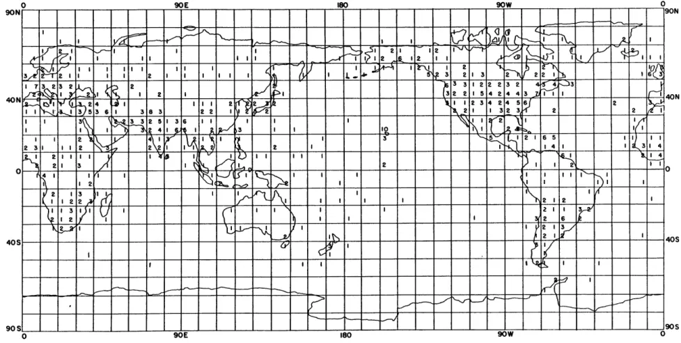
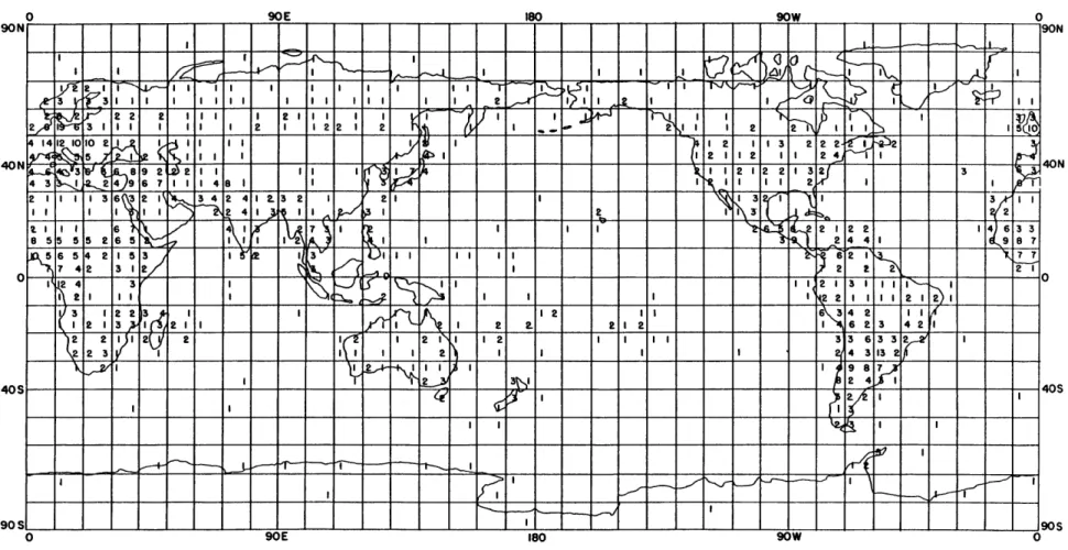
station location, sources, altitude, and so forth are also included. Maps of the numbers of stations in each 50 x 50 grid square in 1949 and 1972 are given in Figures 1 and 2, respectively. Station coverage appears to increase generally over the period, although some squares do show decreasing numbers of stations. Some land and ship stations are

Figure 1. Number of Stations with Data in Each 50 x 50 Grid Square: 1949. 90N I I ... ,)N

,1

---

,,2_/. -

I,_

""1

-2. .

C ' ,%

I

(

2

3 3

5 1 3-6 1

,2

1

1

40

_{, ,}

" " '

_{I ,}

_,

_,

I

_,

s

I

I

analysis to ensure consistency with other studies. Clearly, there are substantially more stations in the Northern Hemisphere than in the Southern Hemisphere. Geographic coverage in the Southern Hemisphere is

further limited by the high ratio of ocean area to land area.

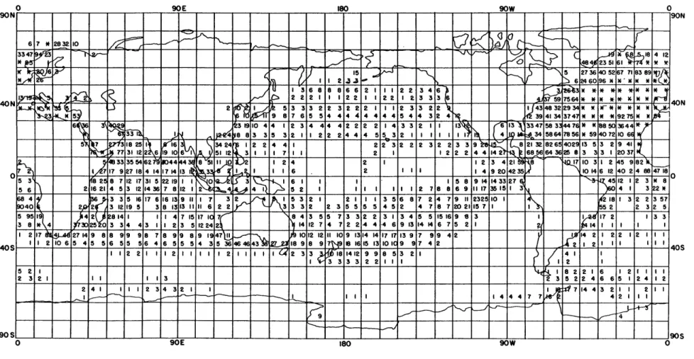
Monthly mean SAT's over the oceans based on ship observations were obtained on magnetic tape from the U.K. Meteorological Office (personal communication, 1978, 1979). Monthly values for 10 x 10 grid squares between 800S and 800N are recorded to the nearest 0.010C along with counts of the numbers of observations per month. Data for December 1962 were incorrect on the original magnetic tape and were dropped from this analysis.

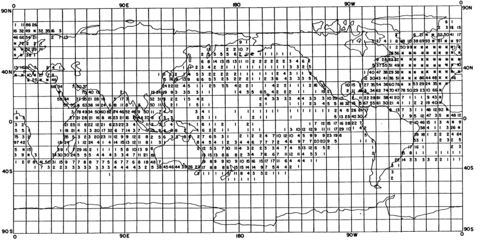
Figures 3 and 4 depict the average number of observations per month in each 50 x 50 grid square over the period 1949-72 for the months Janu-ary and July, respectively. In JanuJanu-ary, reasonably dense coverage is apparent from about 450S to 700N, while in July a small shift in cover-age northward is noticeable. Observations are extremely dense in the North Atlantic and reasonably dense in the Indian Oceans and portions of

the Pacific Ocean. Poor coverage is evident in the tropical and south-eastern areas of the Pacific and in the South Atlantic. Areas north of about 750N or south of about 500S, which make up only about 5% of the

total Northern Hemisphere oceanic area and about 22% of the Southern Hemisphere oceanic area, respectively, contain few observations.

A potentially important deficiency in the marine dataset is the low number of observations per month in many grid squares. The fewer the observations in a particular month, the larger is the potential sampling

Figure 3. Average Number of Temperature Observations per Month in Each Oceanic 50 x 50 Grid Square, 1949-72: January. Asterisks indicate an average of 100 or more observations per month in a grid square.

Figure 4. Average Number of Temperature Observations per Month in Each Oceanic 50 x 50

Grid Square, 1949-72: July. Asterisks indicate an average of 100 or more

observations per month in a grid square.

90N SON I I I I I - - - - 3 1 N 81 I 22l107 72634 16 I I 2 36 43 3 5 30 993353 ₁₀₇ 45565222 1 2 70477509 23 10 6 S 28 17 2 31 2542 2 2 4 3 12 2 3 4 3 81 5841207 943 S3 618 II 14 8_ _O II I5 I 2 I I II 23 4 5 518 6755613041 1 2 2 1940 3 784 34 0 4 52 9 Ii 2 3 4 I I I I I I I I I I I I 1 I I 2 4 6 26 137 3 r I 48 12 92 P. ,2 .I I I I I i 11 I 1 39 3 48 12 32 12511822 1221632234 i 4 I6112 I 21 741215171628227 4615134*9 55 182143320173671437 8 8 6 2 2 2 II I 3 10 12 12 90 29P 48 47 317 I 5 _{97 P212 4} 6 1 85 1 7 6 53 2 2 3 3 42 21 2 2 4 1 7 1 2 710 2 2 1 6925 41 1 1 5 99 21627 9 23 1946 5 3554 36 60_ 3 5 3 2924 35 I 2 2 2 4 64_ 2 I I A 93 35 339 1 5 1.4 5 5 65 42 2 2 1 12 6 5 2 M 216 04 I 292 063 25 3943 9 5 3 3j 2 I 2 1 4 33 31 43 30 34104421122111 5941207 11 1 9 43 I 2 IT 8 31 I 9 7 7 8 8 7 7 5 6 7 7 6 8 48 1 89 9 1o 9 I156 1517 17 1 64 44 I11 1 3 3 2 2 II S 17 32 23 3333 333444 4325384546 6 17 88 86 5151414 97 5442 I3 44 9 I I 4 I 11 12 29 32 40S 1 I 214 33 2017 32 6 71 i I 7 F A, Q 16 2 1 1 1 13 01154 1 3 6 90 3 3 2 1112 99 2 56 7 65 31 2 4 711210 415 99 93196 1 181 22 214 905 -- - - - - - - ---0 90E 9OW MtE 90W

error due to local, short-term temperature fluctuations within the month. However, omission of the grid squares with limited observations would

entail substantial loss of geographical coverage, as evident from Figures 3 and 4, and indeed might introduce biases arising from the resulting preponderance of grid squares near coasts. On the other hand, the pre-sence of significant daily auto-correlation, as found by several analysts for SAT and SST data (Newell, personal communication, 1981; Wigley, per-sonal communication, 1981; see also, Madden, 1977), should decrease the sampling error considerably. Moreover, by averaging together many grid squares, the error should be reduced by at least a factor of the square root of the number of grid squares (assuming simplistically that the sampling error is the same in all grid squares and that these squares are not spatially correlated). Thus, although the time series for indi-vidual grid squares may be subject to large sampling error, the net error in time series for zones, regions, and the globe as a whole should be relatively less. Also, any such sampling errors would likely contri-bute only to the "noise" already present in the data, and not distort any "signal" (assuming that the errors are unbiased and random). In

this analysis, grid squares with two or more observations per month are retained.

Analysis Procedure

Two primary objectives in this study were to develop:

a) consistent time series for land and sea SAT's, separately and in combination; and

b) time series comparable with previous studies.

series averaged over zones (50-wide latitude bands), regions (the trop-ics and extra-troptrop-ics and the hemispheres), and the globe as a whole. The monthly time series can be used for detailed comparisons of land and

sea data on monthly and seasonal time scales, while the annual data are more suitable for examination of long-term trends, especially as com-pared with other studies. The zonal time series permit close

examina-tion of the distribuexamina-tion of temperature change by latitude. The region-al and globregion-al time series give an indication of the overregion-all behavior of large areas of the globe.

The steps taken to generate monthly and annual time series for both land and oceanic data and for zones, regions, and the globe are summar-ized in equation form in Table III. Sections A and B of this table il-lustrate the procedures used for, respectively, the monthly and annual time series for the land-based (NCAR) data; sections C and D the proce-dures for the sea-based (UK) data; and sections E and F the procedures for the combined land/sea data. Small letters in this table indicate monthly values; capital letters indicate annual values. Marine data are distinguished by a single apostrophe, and combined land/sea data by a double apostrophe. Variable names and subscripts are defined in the table.

As noted in the previous chapter, most analysts derive anomaly values of temperature relative to the mean values of some base period to permit consistent averaging of station data. In this study, anomalies are generated from all available data for each station or 50 x 50 grid square during the period 1949-72 (eqns. Al, B2, C2, and D2). This

Table III. Equations Used in This Analysis.

Land-Based (NCAR) Station Data

Monthly Analysis (Equations Al - A4)

t

Sa.

1m

Annual Analysis (Equations Bl - B5)

:5 t ij _k Bl Tjk = i 1k 12 A. jk = Tjk- jTSTjk

2_1

Jn

for each month i, year j, and station k with data.

for each month i and year j and all stations k with data in each grid square 1.

for each month i and year j and all grid squares 1 with data in each

latitude band m (weighted by land area in each grid square 1).

for each month i and year j and all latitude bands m with data in each region (or globe) n (weighted by

land area in each band).

for each year j of each station k with at least i=ll months of data (up to one missing month interpol-ated).

for each year j and station k with data.

for each year j and all stations k with data in each grid square 1.

for each year j and all grid squares 1 with data in each lati-tude band m (weighted by land area in each grid square).

for each year j and all latitude bands m with data in each region

(or globe) n (weighted by land area in each band).

Al

A2

A4

Table III (continued)

Sea-Based (UK) Data

Monthly Analysis (Equations Cl - C4)

. tijk* Cl _{tij = k*} -

i31

j

_z'.. *w'

for each month i and year j and all 10 x 10 grid sguares k* with data in each 50 x 5 grid square 1. for each month i, year j, and grid square 1 with data.

for each month i and year j and all grid squares 1 with data in each latitude band m (weighted by sea area in each grid square).

for each month i and year j and all latitude bands m with data in each region (or globe) n (weighted by

sea area in each band). Annual Analysis (Equations D1 - D4)

Dl T' - 31 = t ijl 12 D2 G! T -

j

i

for each year j of each grid square 1 with at least i=ll months of data (up to one missing month interpol-ated).

for each year j and grid square 1 with data.

for each year j and all grid squares 1 with data in each lati-tude band m (weighted by sea area in each grid square).

for each year j and all latitude bands m with data in each region

(or globe) n (weighted by sea area in each band).

Table III (continued)

Combined Land/Sea Data

Monthly Analysis (Equations El and E2)

(z.- w) + (z' *W') El z . = Im m 1 m m -- im :W W J w + w m m 1 z'.'. * w" E2 r'.'. .. 3m m -- in W" Sm m

Annual Analysis (Equations Fl and F2) SZ" (Z. * W ) + (Z * w') Fl Z.m m 3m m -- 3m w + w m m F2 R = m 3m m m

for each month i, year j, and latitude band m with both land and sea data (value set to z if z' is missing and to z' if z is missing).

for each month i and year j and all latitude bands m with data in each region (or globe) n (weighted by total land and sea area in each band).

for each year j and latitude band m with both land and sea data (value set to Z if Z' is missing and to Z' if Z is missing).

for each year j and all lati-tude bands m with data in each region (or globe) n (weighted by total land and sea area in each band).

Key:

temperature value- (absolute; oC) anomaly value:f dra1ndsstation -k

anomaly value for a 50 x 50 grid square 1 anomaly value for a 50-wide latitude band m anomaly value for a region (or globe) n proportion of land, sea, or total area in a or latitude band m

indicates sea data

indicates combined land/sea data

grid square 1 Note: wi" = + ; w 21; 1 1 1 _{m 11} w' = w'; m 11 t,T a,A g,G z,Z r,R W1 m wmI = w" m ₁

approach minimizes the omission of station data due to incomplete

records during a base period and has the added advantage that the anoma-ly values over the period of anaanoma-lysis sum to zero (within rounding er-rors). However, a disadvantage is that as new data are added, the entire time series must be recomputed.

Monthly anomalies were calculated by subtracting the long-term monthly average from each monthly value, thereby automatically removing the mean seasonal cycle (eqns. Al and C2). Annual anomalies were derived from the monthly data by first calculating annual (calendar-year) values at each land station or 50 x 50 oceanic grid square (eqns. BI and Dl). A linear interpolation was performed if a single monthly value was

mis-sing in a year. Years with more than one month mismis-sing were excluded. The annual time series thus contain slightly less station information

than the monthly time series. A long-term annual mean was then calcu-lated and subtracted from the annual values to form anomalies (eqns. B2 and D2).

To minimize biases due to the highly variable density of land sta-tions, time series of station anomalies within the same 50 x 50 grid square were averaged together (eqns. A2 and B3). Equal weight was given to each station regardless of its exact location within the grid square, since many squares contain only one station and tests with alternative weighting algorithms showed little difference in results.

In the case of the sea data, the means for 10 x 10 grid squares supplied by the U.K. Meteorological Office were averaged together into

after the derivation of anomaly values (eqns C2 and D2). This proce-dure increases the likelihood of continuous time series within each 50 x 50 grid square.

Zonal means for land and sea data were derived by averaging all available grid squares weighted by the proportion of land or sea area in each grid square (to the nearest 10%; eqns. A3, B4, C3, and D3). To form combined land/sea time series for each zonal band, the individual land and sea time series for the band were averaged together weighted by the overall proportion of land versus sea in the latitude band (eqns.

El and Fl). When either land or sea data were missing, the combined

value was set to the remaining value. The weights used in all of these computations agree closely with the land/sea percentages given by

Taljaard (1972).

Time series for regions and the globe as a whole were then calcu-lated from all available zonal means weighted according to the land, sea, or total area in each zonal band (eqns. A4, B5, C4, D4, E2, and F2). The regions used were the northern extra-tropics (200N - 900N),

the tropics (200S - 200N), the southern extra-tropics (900S - 200S), the Northern Hemisphere (0O - 900N), and the Southern Hemisphere (900S

- 00). Global means include all available latitude bands between 900S

and 900N (see Figure 5).

The use of zonal means to form global and regional time series has two major advantages over other possible methods (e.g., averaging of all available grid squares). First, this procedure permits a more

Number of Latitude Bands in the Hemispheres and the Globe with Combined Land/Sea Data, 1949-72. 1945

1950

1955

1960

1970

1980