HAL Id: hal-02001387
https://hal.archives-ouvertes.fr/hal-02001387
Submitted on 31 Jan 2019
HAL is a multi-disciplinary open access
archive for the deposit and dissemination of
sci-entific research documents, whether they are
pub-lished or not. The documents may come from
teaching and research institutions in France or
abroad, or from public or private research centers.
L’archive ouverte pluridisciplinaire HAL, est
destinée au dépôt et à la diffusion de documents
scientifiques de niveau recherche, publiés ou non,
émanant des établissements d’enseignement et de
recherche français ou étrangers, des laboratoires
publics ou privés.
Improving multiphase induction-heating systems:
several configurations and resonant control show promise
Quoc Dung Phan, Anh Tuan Vo, Thang Pham Ngoc, Pascal Maussion
To cite this version:
Quoc Dung Phan, Anh Tuan Vo, Thang Pham Ngoc, Pascal Maussion.
Improving multiphase
induction-heating systems: several configurations and resonant control show promise. IEEE
Indus-try Applications Magazine, Institute of Electrical and Electronics Engineers, 2018, 24 (2), pp.45 -66.
�10.1109/MIAS.2017.2740452�. �hal-02001387�
OATAO is an open access repository that collects the work of Toulouse
researchers and makes it freely available over the web where possible
Any correspondence concerning this service should be sent
to the repository administrator:
[email protected]
This is an author’s version published in:
http://oatao.univ-toulouse.fr/21456
To cite this version:
Phan, Quoc Dung and Vo, Anh Tuan and Ngoc, Thang Pham
and Maussion, Pascal Improving Multiphase
Induction-Heating Systems: Several Configurations and Resonant
Control Show Promise. (2018) IEEE Industry Applications
Magazine, 24 (2). 45 -66. ISSN 1077-2618
Official URL:
https://doi.org/10.1109/MIAS.2017.2740452
This arTicle presenTs a new configuraTion for mulTiphase induction-heating (ih) systems and their control schemes. instead of using separate voltage inverters to supply the required current to the inductors in each phase, we specifically configured the inverters to reduce the number of power switches. a modification of the inverter-setting parameters ensured the proper operation of the system. we obtained the best references through a specific opti-mization procedure and tested several solutions for neutral current miniopti-mization, including a new arrangement of the coils. in addition, proportional-resonant (pr) controllers allowed us to achieve current con trol in the different phases. we developed the application on a reduced-power, three-phase coupled resonant test bench, which provided simulation and experimental results.
This Technology’s Time Has Come
ih is a good industrial technique for many applications, such as metallurgical heat treatment, drying, degreasing, stripping, merging, and galvanizing, and is even used in the food industry [1], [2]. it has many advantages when compared to classical heating solutions, such as flame heating, resistance heating, and tra-ditional ovens and furnaces. high-power density can be achieved with flexibility, high energy efficiency, speed, no gas emissions, and no local waste; contactless heating of metallic parts is also possible.
an increase in the power and power density in the heated work piece can be accomplished using multiphase solutions. such systems include several inductor coils supplied by a number of current or voltage inverters to obtain a required temperature profile in the piece to be heated. multiphase ih generators could
By Quoc Dzung Phan, Anh Tuan
Vo, Thang Pham Ngoc, and
Pascal Maussion
Improving Multiphase
Induction-Heating Systems
involve multiple inductors [3], [4], where the flux distribu-tion is achieved with flux concentrators and moving mag-netic screens. in addition, more flexible and cost-effective architectures have been proposed [5]–[11] that have no moving parts thanks to power electronics, by which an accurate control of the heat profile can be implemented through the phase current control.
in classical solutions that deal with the control of multi-phase ih systems, separate voltage or current inverters are used to drive the current in each inductor for longitudinal flux [5], [6] and transverse flux [7]. nevertheless, some innovative solutions have been proposed for reducing the number of power switches. an interesting topology com-posed of a three-phase series-resonant inverter, matching transformers and capacitor filters, and an ih balanced load has been described in [8]. a dual-resonant half-bridge volt-age inverter supplies a double coil in [9], but this solution does not seem to be adapted for more than two phases. a structure with four switches, two capacitors, and one transformer with two primary windings and one second-ary winding is studied in [10], but it is limited to a single load. multiple-output power converters are arranged in a series-resonant multi-inverter topology in [11]–[14], but this occurs mainly in the field of home appliances. never-theless, whatever the architecture of multiphase systems, there is high complexity that is mainly due to interactions between the converter, the inductor, and the heated piece, which makes modeling and control rather difficult.
in this article, we optimize the power supply and reduce the number of switches by forming an n-phase
power supply that includes (n 1+ ) legs of power switches
in parallel. as in similar cases, phase currents in the dif-ferent phases are controlled through pr controllers, which are a powerful solution for eliminating the tracking error that originates from sinusoidal reference signals.
Description of the Three-Phase IH System
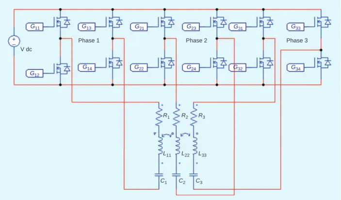
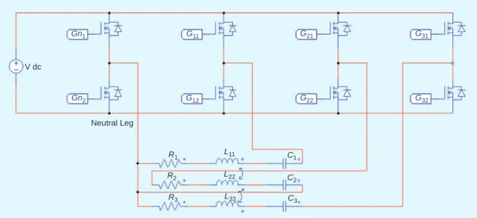
figure 1 describes the architecture of a classical voltage inverter arrangement where each phase is connected to its own inverter. The total number of switches reaches 2n. figure 2 describes the architecture of the proposed origi-nal multiphase inverter configuration. here, a common leg, called the neutral leg, will be combined with each phase leg to supply the current in each phase. Thus, the number of legs and switches will decrease by (n − 1). This system, therefore, will use 2(n − 1) fewer power switches than the previous one.
for the proof of validity that is the aim of this article, we built a low-power, three-phase ih system to emulate the electrical part of that type of system, as in [15]. This test bench was composed of independent voltage inverter legs with a common dc source, dead times, and thermal shut-down. each phase included a resonant capacitor in serial association.
The inverter load in figure 3 consists of three inductors organized in a serial configuration with u- and i-shaped ferrite cores with small air gaps. The technical param-eters of this test bench are expressed as a 48-V maximum dc voltage, a wide range of switching frequencies up to 100 khz, and a 5-a maximum current. The impedance
G11 G13 G14 G22 G21 G23 G31 G32 G34 G33 G24 G12
Phase 1 Phase 2 Phase 3
V dc + – R1 R2 R3 L11 L22 L33 C1 C2 C3
parameters of this three-phase inductive circuit are listed in Table 1. an automatic parameter identification procedure has been proposed in [15].
a matrix model of the system is given in (1), where sinusoidal currents I1, I2, and I3 feed the three coils
through the inverters. it has been extensively described in [16]. . j V V V R jL jM jM jM R L jM jM jM R jL I I I LR1 LR2 LR3 1 1 21 31 12 2 2 32 13 23 3 3 1 2 3 ~ ~ ~ ~ ~ ~ ~ ~ ~ = + + + r r r r r r
>
H
>
H H
>
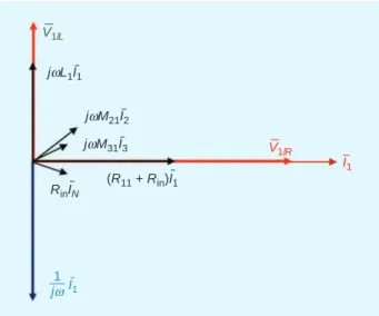
(1)a vector diagram of the first phase of the proposed configuration is shown in figure 4. The voltage drop in the switches for this configuration is different from the classical one because of its common leg. The current flow
through this leg is IN, which is the sum of all three phase
currents.
capacitor banks have been calculated based on the diagram in figure 4 to compensate for the reactive power in the three phases and create a resonant circuit in each. The calculation, which does not take into account the effect of the neutral current, is expressed as
. cos cos C1 L I M I I M I 1 1 12 12 2 13 13 3 1 ~ ~ ~ { ~ { = + + ^ h (2)
Temperature Profile Optimization Procedure
The first goal of the optimization procedure is to define a set of phase currents, which leads to the predefined power density along the radius of the metal (nonmag-netic) disk cross section. The second objective is to minimize the amplitude of the neutral current in the neutral leg. The approach is based on the power-densi-ty distribution functions of the induced currents on the disk, as shown in figure 5 and intensively described in [16]. The calculation of the total induced current
FIGURE 3.
The three coupled coils on the reduced-power test bench.V dc + – Gn1 Gn2 G11 G12 G21 G22 G31 G32 R1 R2 R3 L11 L22 L33 C1 C2 C3 Neutral Leg
FIGURE 2.
The architecture of the new IH system (so-called three direct legs) with only four legs, eight switches, serial capacitors, and coupled inductors.i/j
1
2
3
R (Ω) 1 2.27 0 0 L (mH) 2.93 0.086 0.027 R (Ω) 2 0 2.44 0 L (mH) 0.086 3.15 0.171 R (Ω) 3 0 0 2.74 L (mH) 0.027 0.171 2.86density, where index k = 1, 2, 3 denotes the inductor k, is expressed as , . J x A f x I f x I j f x I f x I k kR kR kI kI k kR kI kI kR 1 3 1 3 disk = -+ + = =
/
/
^ ^ ^ ^ ^ h h h h h 6 6 @ @ (3)in (3), fkR(x) is the real part of the image of induced
cur-rent k at the abscissa x, and fkI(x) is the imaginary part.
The value IkR is the real part of the current Ik, and IkI is
the imaginary part. finally, Rdisk is the radius of the disk,
and x is the position along it, with 0 < x < Rdisk.
The next expression,
, ,
DP x X^ , h=tdisk diskJ2 ^x Xh (4)
gives the calculation of the total power density at each abscissa along the radius. it is a nonlinear equation with
five variables that are the amplitudes and the phase angle of the three phase currents. This equation can be solved in an optimization procedure by finding the minimum of a cost function, such as the following, with the addition of many constraints: [ , , , , ], ( , ) . X I I I F D x XD D p p p 1 2 21 3 31 ref { { = = - ref (5)
in the classical configuration with 12 switches, where the inverters are independent, constraints for the cost func-tion could be expressed as
, , . A I F F k 0 5 180 180 1 1 2 3 max k k1 c c # # # # # { -= = Z [ \ ] ] ]] (6)
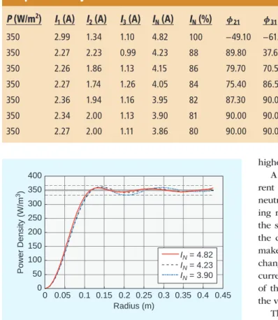
Table 2 lists the best solutions obtained from the maTlaB optimization program for a range of power densities. The maximum power-density value is obtained when the optimized residue value reaches its maximum value Fmax. figure 6 shows the relation between the power
density and its optimized residue value. we see that, from the inertial point to the power density of 350 w/m3,
the residue values are all constant and current profiles have the same phase angle and amplitude values, which change as follows: . ID ID DD P P 1 2 = P2 P1 (7)
after that range, all of the constraints almost reach their limits, optimized residue values increase, and current pro-files change without following any rule.
in fact, if the optimized residue does not change and the relative current profile obeys the rule of (7), as the power density changes, the values of the capacitors
0 –5,000 –10,000 –15,000 0 –5,000 –10,000 –20,000 –15,000 0 0.1 0.2 0.3 0.4 Rayon (m) 0 0.2 0.4 Rayon (m) (a) (b) f1R (1/m2) f2R (1/m2) f3R (1/m2) f1I (1/m2) f2I (1/m2) f3I (1/m2)
FIGURE 5.
The distribution functions of the induced current: the (a) real (R) part and (b) imaginary (I) part, at 1,500 Hz and an ambient temperature of 20 °C. V1/L V1/R I1 jωL1I1 RinIN jωM21I2 jωM31I3 (R11 + Rin)I1 1 jω I1as shown in (2) are also constant. for an ih system that operates over a wide range of power densities, this requirement is crucial. Thus, we should choose a cur-rent profile that is a compromise between a wide power-density range and an adequate residue to apply to the system. in this case, we need to use the optimized power-density profile of 1,800 w/m3, the residue value of which
is 0.59. The current profile of another power density can be inferred from (7), and the system capacitor values are
. , . , . F
3 78 3 41 3 72 n
6 @ .
as mentioned in the section “Description of the Three-phase ih system,” the method to control the switching states of the eight switches in the new con-figuration is somewhat more complex. The use of a com-mon leg restricts the alternating capability of the power switches on the other legs. This leads to a limit on the current phase angles in a switching zone instead of the four-quadrant zone, as in the classical configuration. moreover, constraints regarding power-switch switching zones must be considered in the optimization program. These constraints are defined by characteristic angles and current phase angles:
, , . A I F F k 0 5 0 90 1 1 2 3 max k k k k k k 1 0 1 0 0 1 c c # # # $ # # # # { a a { a a a a a -- -= = Z [ \ ] ] ] ] ] ] ]] (8)
characteristic angles ai can be identified through the phase
current, the impedance of the load, and the amplitude of the fundamental harmonics of the phase voltage. moreover, a special angle a0 is added to the constraints to shift the
power-switch switching zones to more beneficial zones for
optimizing the residue. at the initial point of the maTlaB program, a0 is set to 0°; after that, it is linearly changed on
both sides of the 0° to determine whether there is a better current profile. The value of a0 is flexible, but its absolute
value is always less than a1 to ensure that the switching
sig-nal on the first phase can be implemented.
one more constraint that has to be taken into account is the maximum current that flows into the neutral phase, which is the vector sum of the three phase currents, as shown by
.
IN=I1+0c+I2+{21+I3+{31 (9)
The neutral phase current has been continuously reduced until the residue of the best solution of the cost function has reached the threshold value Fmax. These constraints
are all nonlinear and commonly difficult to calculate. however, powerful maTlaB tools such as fmincon can solve this problem quickly and effectively.
several solutions obtained from the maTlaB optimiza-tion program for a 350-w/m3 reference power density are
listed in Table 3. Three solutions for three typical cases are shown in figure 7. The best-fitting line is the solid red line, where the residue is the smallest but the neutral phase current is the highest. The black dashed line shows that the neutral phase current is 12% less than in the previous one, and the residue is still below the residue threshold value, which leads to a lower percentage error around the target. finally, the neutral phase current is minimized, 18% less than in the first case, and the tracking error is slightly higher than in the second case but still small enough, as represented by the blue dashed curve. in reality, depending on the purpose of the application in terms of using a high, precise heat treatment or not, we can choose one of these three compromises to achieve the desired effectiveness.
phasor diagrams of the first and second current profiles are shown in figure 8. all of the current vectors are in their switching zones. for the first case, the special angle
0
a is equal to zero, but for the second case, it is set as .a1
Table 2. A list of solutions for the classical
configuration following the power density
Power
Density
(W/m
3)
I
1
(A)
I
2(A)
I
3(A)
U21 U31Residue
300 2.77 1.24 1.02 −49.10 −61.05 0.21 350 2.99 1.34 1.10 −49.10 −61.05 0.21 500 3.57 1.60 1.32 −49.10 −61.05 0.21 700 4.23 1.89 1.56 −49.10 −61.05 0.21 750 4.34 1.91 1.63 −48.53 −57.41 0.21 950 4.45 1.92 1.96 −35.43 −32.61 0.38 1,000 3.79 3.38 1.77 82.27 54.27 0.41 1,400 4.47 3.52 2.39 75.05 74.80 0.44 1,950 4.82 3.65 2.85 51.44 50.94 0.93 2,000 4.82 3.68 2.88 49.05 48.72 1.11 0.00 0.20 0.40 0.60 0.80 1.00 200 400 600 800 1,000 1,200 1,400 1,600 1,800 2,000 Residue Power Density (W/m3)
FIGURE 6.
The relation between the power density and its optimized residue value of the classical configuration.Neutral Current Reduction
The apparent advantage of our new power supply con-figuration is the reduction in the number of switches, which leads to lower weight and reduced price. never-theless, there is always a tradeoff. in this case, the use
of a common leg for all of the phases causes the current flow in this leg (the neutral current) to be the sum of the currents in each phase. The risk is that this sum could become higher than the phase currents, leading to special sizing. in this system, we used the optimization program to prove that the residue will be low enough if the phase current vec-tors are all in the same quadrant of the phase plane (quadrant 1 or 4). Therefore, the amplitude of the neutral current will always be higher than the one of three phases.
a new original configuration is the change in the cur-rent direction inside one of the n phases to reduce the neutral current, as shown in figure 9. The correspond-ing reference current must also be inverted to maintain the same flux direction in the coils. we chose to inverse the connections of phase 2 and its reference current to make the neutral current equal to IrN=Ir1+Ir2l+r without I3
changing the flux produced by coil 2, Ir2l= -Ir . now, the 2
current vectors of I2l and I3 are in two opposite quadrants
of the phase plane (4 and 2, or 1 and 3). consequently, the value of IN will decrease significantly.
Theoretically, the amplitude of the neutral current will decrease, but, to obtain the relative profile current, we must be able to control the power switches according to constraints such as those in (8). for instance, by reusing the first current profile in the section “Description of the Three-phase ih system” and reversing the direction of the second-phase current, we have the phasor diagram as illustrated in figure 10(a). The neutral current amplitude is just 2.65 a, and, although the angle a0 has been tuned
to its limit, the vectors represented by the solid blue and green lines are both not in their switching zones. There-fore, we cannot simply reverse a phase current direction and continue to use the current profile, as solved in the “Description of the Three-phase ih system” section. The optimization procedure must now be implemented with new constraints, which are expressed as
, , . I A F F k 0 5 180 180 0 90 1 1 2 3 max k k 21 2 0 21 2 0 31 3 0 31 3 0 0 1 c c c c # # # $ # $ # # # # { a a { a a { a a { a a a a a - -- -- -= = Z [ \ ] ] ] ] ] ]] ] ] ] ] ] ]] (10)
Then, a new current profile is found, the phasor diagram of which is in figure 10(b). The reference
Radius (m) 0 0.05 0.1 0.15 0.2 0.25 0.3 0.35 0.4 0.45 Power Density (W/m 3) 0 50 100 150 200 250 300 350 400 IN = 4.82 IN = 4.23 IN = 3.90
FIGURE 7.
The power-density optimization along the radius for three typical cases.IN
Second-Phase Switching Zone Third-Phase Switching Zone Not a Switching Zone
I1 I2 I3
(a) (b)
FIGURE 8.
The switching zones of two current profiles: (a) IN = 4.82 A;(b) IN = 4.23 A.
P (W/m
2)
I
1
(A)
I
2(A)
I
3(A)
I
N(A)
I
N(%)
z21 z31Residue
350 2.99 1.34 1.10 4.82 100 −49.10 −61.05 0.21 350 2.27 2.23 0.99 4.23 88 89.80 37.60 0.39 350 2.26 1.86 1.13 4.15 86 79.70 70.50 0.43 350 2.27 1.74 1.26 4.05 84 75.40 86.50 0.46 350 2.36 1.94 1.16 3.95 82 87.30 90.00 0.65 350 2.34 2.00 1.13 3.90 81 90.00 90.00 1.07 350 2.27 2.00 1.11 3.86 80 90.00 90.00 2.18
Table 3. A list of different solutions for the proposed original configuration at
the power density of 350 W/m
3value of this profile is X = [2.96 A, 1.17 A, −57.3°, 1.22
A, −36.7°]. The neutral current of this profile is 3.31 a.
consequently, the neutral current amplitude has been significantly reduced (31%, as compared to the first pro-file), and the power switches in the neutral leg do not need to be oversized when compared to the phase-leg switches.
additionally, because of the limits of the switching zones, we cannot continue to use the current profile in the “Description of the Three-phase ih system” section and simply reverse one of the phase currents to reduce the neutral current. in fact, power-switch switching zones directly depend on the first harmonic of the phase volt-ages and not on the phase currents. accordingly, the problem with switching zones can be solved by modifying capacitor values. instead of tuning capacitor values to have resonant phenomena in all three phases, these values can be changed to create the difference in phase of the phase currents and their relative phase voltage first harmonics. Therefore, we can keep the current phase angles, and the voltage phases are suitable for the switches to work. The new capacitor value of in-phase i can be proven as follows:
. tan Ci 1 C RC i i i 2 ~ d = + l (11)
in this expression, Ci is the old capacitor value, Ri is the
resis-tive part of the load, and dk is the phase difference between
the phase current and the first harmonic of the phase voltage. By modifying the optimization program, the new val-ues of the capacitors can be calculated for a wide range of power densities. however, the capacitor values’ depen-dence on loads is not appropriate for industrial require-ments. if the ih system operates with a metal disk, the dimension, depth, and material of which are not much changed, then this method can be used efficiently.
Gn1 Gn2 Gn11 Gn12 Gn21 G31 G32 Gn22 V dc + – Neutral Leg R1 R2 C1 C2 R3 C3
FIGURE 9.
The architecture of the modified new IH system, with only four legs, eight switches (two so-called direct legs plus one invert leg), serial capacitors, coupled inductors, and a reduced neutral current.(a) (b)
IN
Second-Phase Switching Zone Third-Phase Switching Zone Not a Switching Zone
I1 I2 I2′ I3
FIGURE 10.
The switching zones of two current profiles: (a) the inverse version of the first profile in the section “Temperature Profile Optimization Procedure” and (b) the optimized profile of the new configuration with phase inversion.Power-Density Range of Each Configuration
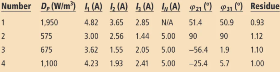
another aspect worth investigating in the optimization procedure is the comparison of the maximum power density obtained by the new and previous configura-tions within the given constraints in (8) and (10). The reference power density will be linearly increased, and the constraints will be sequentially applied. This leads to the limits listed in Table 4 for each configuration. con-figuration 1 is the classical solution (figure 1), with 12 power switches, where each of the three phases is sup-plied by its own inverter. solution 2 in Table 4 is present-ed in figure 2, with only eight switches, serial capacitors, and coupled inductors. solutions 3 and 4 are improved versions of solution 2 and were described in the “neutral current reduction” section for a special neutral current reduction.
There is a significant difference in the power density of these four configurations. without the nonlinear con-straints, the maximum power density obtained by the classical configuration is far better than the new one. This result points to an inconvenience of the reduced configu-ration, but the improved arrangement and the change in capacitor values described in the “Temperature profile optimization procedure” section dramatically reduce its effect. The change in direction of the second-phase cur-rent helps to lower the neutral curcur-rent, and the change in capacitor values helps to make the phase current angle constraints more flexible, so the power-density range increases significantly.
as mentioned in the section “Temperature profile opti-mization procedure,” the optiopti-mization program will find the best current profile for each power-density value. however, when the power-density value increases to the saturation value, the residue will also increase, and the current profile will change without following any rule, as in
(7). This leads to a change of the capacitor values. accordingly, we should choose the current profile to have a wide range of power density, as described in the “Description of the Three-phase ih system” section. Table 5 shows a stable power-density range and the chosen current profile and capacitor values of each configuration at a power density of 350 w/m3.
we can deduce the current profile of other power-density values in this range from (7).
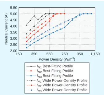
figure 11 shows the neutral cur-rent of three new configurations with two current profile selection methods. The solid lines represent the best-fitting current profiles of each power-density value, and the dashed lines represent the current profiles that keep capacitor values constant in a wide range of power densities.
PR Controller
we optimized the reference current vector through a specific procedure with a flat temperature profile in the heated metal sheet objective. as a consequence, the con-trol loops have to adjust the characteristic angles ak and dk
to force the current to follow the references.
as the reference is an ac variable having a nonzero frequency, the kind of control loop in this ih system can-not be properly built using standard proportional-integral controllers, because they only cancel steady-state errors (for ~=0). other controllers have to be used to cancel a sinusoidal tracking error. amplitude modulation, such as park’s transformation, can help to resolve the problem with the ac reference. however, the global control scheme will be more complex and have a high computational bur-den. Therefore, other solutions should be envisioned.
resonant controllers were initially proposed by [18]. They are well known for their interesting properties when sinusoidal reference tracking is required. reso-nant controllers can achieve high performance in both multisinusoidal reference tracking and disturbance rejection due to an infinite gain at the fundamental frequency. The recent literature presents several power-electronics applications of resonant control, e.g., for a seven-leg back-to-back converter for supplying variable-speed generators in [19] and stand-alone voltage source inverters in [20].
The general form of a resonant controller can be expressed in the s-domain as
, G s s s K s 2 2 r 2 r 0 02 0 p~ ~ p~ = + + ^ h (12)
where ~ is the frequency to track and p is a
damp-ing factor (set close to zero in this type of controller).
Number
D
P(W/m
3) I
1(A)
I
2(A)
I
3(A)
I
N(A)
{21(°)
{31(°) Residue
1 1,950 4.82 3.65 2.85 N/A 51.4 50.9 0.93
2 575 3.00 2.56 1.44 5.00 90 90 1.12
3 675 3.62 1.55 2.05 5.00 −56.4 1.9 1.10
4 1,100 4.23 1.93 2.41 5.00 −25.4 5.7 1.00
Table 4. The maximum power density obtained by three configurations
compared to the classical one
Number
D
(W/m
PRange
3)
I
(A)
1I
(A)
2I
(A)
3I
(A) Residue
NC
(µF)
1C
(µF)
2C
(µF)
31 550 2.3 2.0 1.5 4.0 0.52 3.76 3.51 3.80
2 650 2.7 1.3 1.7 4.0 0.58 3.78 3.46 3.76
3 1,000 2.6 1.5 1.9 3.6 0.57 3.77 3.20 3.80
Table 5. The solutions for each configuration to obtain the widest
power-density ranges
a proportional control action must be included to achieve appropriate performance. This is the pr controller and is expressed as . G s K s s K s 2 2 p 2 r 0 02 0 p~ ~ p~ = + + + ^ h (13)
a resonant circuit can be physically implemented using active and passive components such as opera-tional amplifiers (Tl074), resistors, and capacitors [21]. in this article, the resonant circuit is made similarly to a second-order bandpass filter, so its center frequency is referred to as the resonant frequency, and its damp-ing factor is low to assure the selectivity of the circuit. The transfer function of the resonant circuit in figure 12 is given by H s s CR s R R R C R R CR s 2 1 1 a b a b a 2 2 2 2 = -+ + + ^ h . (14)
By setting the values of the resistors and capacitors, the resonant frequency fo and the damping factor
g of this circuit are tuned to be 1,500 hz and 0.05,
respectively.
The output of the resonant circuit will be led to a modulator circuit composed of comparators (lm361) and logical integrated circuits (ics) (sn7400). as described in the “gate signals generation” section, two
Vinv Vinv_1 Gi 11 Gi 12 Gn Gi 0 0 0 0 0 0 0 0 0 0 1 1 1 1 1 1 1 1 1 1 11 11 1 1 11 1 11 1 Time
FIGURE 15.
The gate signals generated by the modulator.2.00 2.50 3.00 3.50 4.00 4.50 5.00 5.50 150 350 550 750 950 1,150
Neutral Current (A)
Power Density (W/m3)
IN 1 Best-Fitting Profile
IN 1 Wide Power-Density Profile
IN 2 Best-Fitting Profile
IN 2 Wide Power-Density Profile
IN 3 Best-Fitting Profile
IN 3 Wide Power-Density Profile
FIGURE 11.
The relationship between the neutral current and power density of different configurations and methods of profile selection.Vin Vout R2 Rb Ra C C + –
FIGURE 12.
The analog implementation of the resonant circuit schematic. 5 0 –5 0.034 0.0345 0.035 Time (s) 0.0355l1 l2 l3 lref1 lref2 lref3 IN
FIGURE 13.
The simulated phase and neutral currents with the new IH system (with three direct legs) and an optimized neutral current (4.5 A). 3 0 1 2 –3 –2 –1 0.03 0.0305 0.031 Time (s) 0.0315 0.032l1 l2 l3 lref1 lref2 lref3 IN
FIGURE 14.
The simulated phase and neutral currents with the modified new IH system (with two direct legs plus one invert leg) and reduced neutral current (2.5 A).dc voltages will be compared to the output of the reso-nant circuit to generate gating signals. finally, gating signals will be used to control the switching state of the switches. in the experimental test bench described in this article, we built an analog control board, in which the gain factors Kp and Kr could be adjusted
using variable resistors. although general tuning rules can be found in [22] and [23], they do not take into account simultaneous reference tracking and distur-bance rejection. as a consequence, pr controllers will be tuned by trial and error. Therefore, figures 13 and 14 present the simulated phase and neutral currents for the new ih system with three “direct” legs that are
relatively without and with phase inversion. The neu-tral currents for these two cases are 4.82 a and 3.31 a, respectively.
To convert the pr controller’s output to the switching signals, we developed a modulator based on comparators and logic gate ics.
Gate Signals Generation
The resonance effect of an lc circuit at the fundamen-tal frequency provides a nearly pure sinusoidal form of phase currents, a no-phase difference, and an ampli-tude dependence between this current and the first harmonic of the phase voltage. Therefore, controlling the latter voltage also means controlling the phase cur-rent. a typical phase voltage shape is shown in figure 15, with its first harmonic deduced from
cos sin
Vi1 4Vs t
r a ~ d
= ^ + h. (15)
By changing its characteristic angles a (for amplitude)
and d (for the phase angle), the amplitude and phase of
its first harmonic can be easily adjusted.
To generate a phase voltage shape like Vinv (the red
line in figure 15), two types of control signal are neces-sary. The neutral leg, which is the common leg for all of the the phases, will be controlled by a 1.5-khz pulse with a 50% duty cycle (see the Gn signal). for the other
legs, different gate signals are created, as shown in fig-ure 15. pr controller output can be compared to two dc signals with the same amplitude but opposite sign (the
FIGURE 16.
An analog implementation of a PR controller for the three phases. 0 –10 –20 –30 –40 –50 Gain (dB) Phase (°) 90 45 0 –45 –90 100 500 1 k 5 k 10 k 1 2 3 4 5 6 Frequency (Hz)green lines in figure 15) to create two gate signals Gi11
and Gi12 for leg i. The logic combination for the gate
sig-nal of switch 1 (upper) in leg i can be expressed with a nanD operator, as in
.
Gi= G G Gn i11 i12 (16)
figure 16 shows the analog implementation of these functions.
FIGURE 19.
The reference and experimental current and phase voltage of the third phase and the experimental current of the first phase—configuration without phase inversion.FIGURE 20.
The reference and experimental current and phase voltage of the third phase and the experimental current of the first phase—configuration with phase inversion.FIGURE 21.
The reference and experimental current and phase voltage of the third phase—configuration with phase inversion but without resonance.FIGURE 22.
The experimental current of the first, second, third, and neutral phases—configuration without phase inversion.FIGURE 18.
The reference and experimental current and phase voltage of the first phase—configuration without phase inversion.FIGURE 23.
The experimental current of the first, second, third, and neutral phases—configuration with phase inversion.Experimental Results and Discussion
The pr controllers are implemented with opera-tional amplifiers, resistors, and capacitors. one of their experimental Bode plots is shown in figure 17 as an example, to verify their high gain at the resonant frequency.
Three typical cases for three changes in a power supply configuration have been experimentally verified.
figures 18–21 plot different phase currents when following their sinusoidal reference and some output inverter voltage. indeed, output inverter voltages should theoretically be almost flat at the levels V dc, 0, or –V dc. This is not the case in our system due to the high output resistor value on the small power ic that was cho-sen as the inverter. nevertheless, the system’s behavior is satisfactory, as the currents stick to their references. moreover, the neutral current amplitude of each profile can be easily compared through the voltage drop on the switches. in descending order are figures 19–21, which represent the new configuration 1 without phase inver-sion, configuration 2 with inverinver-sion, and configuration 3 with inversion but without resonance.
figures 22–24 plot the experimental currents on three phases and the neutral phase in three different configura-tions: the new configuration 1 without phase inversion, configuration 2 with inversion, and configuration 3 with inversion but without resonance. The figures show that the neutral current is reduced, as expected.
Conclusions
This article has presented several configurations for multiphase ih systems and their associated and reso-nant control. one specific arrangement of the inverter legs minimizes the number of power switches, which is an obvious advantage. according to an optimization procedure, the power-density profile and the current in the neutral leg could be simultaneously minimized. But a new arrangement of one coil, when its connec-tion and reference current are simultaneously inverted, leads to a significant improvement. The neutral current
becomes almost two times smaller than before, from 4.8 to 2.8 a. consequently, the power switches in the neutral leg do not need oversizing. nevertheless, the maximum power density driven by the system seems to be reduced compared to the classical solution, because of a higher number of constraints for the gate sig-nals. however, due to a change in capacitor value, the power-switches’ switching zones are widened and help the second arrangement to supply higher power den-sity. future work will address the effectiveness of this change, its influence on the resonance of phase circuits, and the power-density range of each configuration.
Author Information
Quoc Dzung Phan is with the ho chi minh city
universi-ty of Technology, Vietnam. Anh Tuan Vo, Thang Pham
Ngoc, and Pascal Maussion (pascal.maussion@laplace
.univ-tlse.fr) are with the université de Toulouse, france. maussion is a senior member of the ieee. This article first appeared as “several configurations and resonant control for multiphase induction-heating systems” at the 2016 ieee industry applications society annual meeting. This article was reviewed by the ias metals industry committee.
References
[1] o. lucia, p. maussion, and D. e. J. Burdio, “induction heating technol-ogy and its applications: past developments, current technoltechnol-ogy, and future challenges,” IEEE Trans. Ind. Electron., vol. 61, no. 5, may 2014. [2] f. sanz, c. sagües, and s. llorente, “induction heating appliance with a mobile double-coil inductor,” IEEE Trans. Ind. Appl., vol. 51, no. 3, pp. 1945–1952, may/June 2015.
[3] s. Zinn and s. l. semiatin, Elements of Induction Heating: Design, Control, and Applications. materials park, oh: asm international, 1988. [4] T. Tudorache and V. fireteanu, “magneto-thermal-motion coupling in transverse flux heating,” COMPEL: Int. J. Computation Mathematics Elect. Electron. Eng., vol. 27, no. 2, pp. 399–407, 2008.
[5] h. n. pham, h. fujita, n. uchida, and K. ozaki, “heat distribution con-trol using current amplitude and phase angle in zone-concon-trol induction heating systems,” in Proc. IEEE Energy Conversion Congress and Exposi-tion (ECCE), 2012, pp. 2474–2481.
[6] Q. Xu, f. ma, a. luo, Y. chen, and Z. he, “hierarchical direct power control of modular multilevel converter for tundish heating,” IEEE Trans. Ind. Electron., vol. pp, no. 99, pp. 1–1, 2016.
[7] m. souley, s. caux, o. pateau, p. maussion, and Y. lefèvre, “optimiza-tion of the settings of multiphase induc“optimiza-tion heating system,” IEEE Trans. Ind. Appl., vol. 49, no. 6, pp. 1–7, 2013.
[8] s. Kleangsin, a. sangsawang, s. naetiladdanon, and c. Koompai, “a power control of three-phase converter with aVfsVc control for high-power induction heating applications,” in Proc. 40th Annu. Conf. IEEE Industrial Electronics Society, 2014, pp. 3220–3226.
[9] f. sanz-serrano, c. sagues, and s. llorente, “power distribution in coupled multiple-coil inductors for induction heating appliances,” in Proc. IEEE Industry Applications Society Annual Meeting, 2015, pp. 1–8. [10] c. Bi, h. lu, K. Jia, J-g. hu, and h. li, “a novel multiple-frequency resonant inverter for induction heating applications,” IEEE Trans. Power Electron., vol. pp, no. 99, 2016.
[11] o. lucía, c. carretero, J. m. Burdío, J. acero, and f. almazan, “mul-tiple-output resonant matrix converter for multiple induction heaters,” IEEE Trans. Ind. Appl., vol. 48, no. 4, pp. 1387–1396, 2012.
[12] i. millán, J. m. Burdío, J. acero, o. lucía, and D. palacios, “resonant inverter topologies for three concentric planar windings applied to domestic induction heating,” Electron. Lett., vol. 46, no. 17, pp. 1225– 1226, 2010.
[13] o. lucía, J. m. Burdío, l. a. Barragán, J. acero, and c. carretero, “series resonant multi-inverter with discontinuous-mode control for improved light-load operation,” in Proc. 36th Annu. Conf. IEEE Industrial Electronics Society, 2010, pp. 1671–1676.
FIGURE 24.
The experimental current of the first, second, third, and neutral phases—configuration with phase inversion but without resonance.[14] Ó. lucía, J. m. Burdío, l. a. Barragán, c. carretero, and J. acero, “pulse delay control strategy for improved power control and efficiency in multiple resonant load systems,” in Proc. 37th Annu. Conf. IEEE Indus-trial Electronics Society, 2011.
[15] B. a. nguyen, Q. D. phan, D. m. nguyen, K. l. nguyen, o. Durrieu, and p. maussion, “parameter identification method for a 3-phase induction heating system,” IEEE Trans. Ind. Appl., vol. 51, no. 6, pp. 4853–4860, 2015. [16] m. souley, s. caux, o. pateau, p. maussion, and Y. lefèvre, “optimiza-tion of the settings of multiphase induc“optimiza-tion heating system,” IEEE Trans. Ind. Appl., vol. 49, no. 6, pp. 1–7, 2013.
[17] J. egalon, K. l. nguyen, o. pateau, s. caux, and p. maussion, “robust-ness of a resonant controller for a multiphase induction heating system,” IEEE Trans. Ind. Appl., vol. 51, no. 1, pp. 1–9, Jan./feb. 2015.
[18] Y. sato, T. ishizuka, K. nezu, and T. Kataoka, “a new control strategy for voltage-type pwm rectifiers to realize zero steady-state control error in input current,” IEEE Trans. Ind. Appl., vol. 34, no. 3, pp. 480–486, may/ June 1998.
[19] r. cárdenas, e. espina, J. clare, and p. wheeler, “self-tuning resonant control of a seven-leg back-to-back converter for interfacing
variable-speed generators to four-wire loads,” IEEE Trans. Ind. Electron., vol. 62, no. 7, pp. 4618–4629, 2015.
[20] a. lidozzi, g. lo calzo, l. solero, and f. crescimbini, “integral-resonant control for stand-alone voltage source inverters,” IET Power Electron., vol. 7, no. 2, 2014.
[21] r. Teodorescu, f. Blaabjerg, m. liserre, and p. c. loh, “proportional-resonant controllers and filters for grid-connected voltage-source convert-ers,” IEE Proc.: Electric Power Appl., vol. 153, no. 5, pp. 750–762, 2006. [22] l. f. alves pereira and a. s. Bazanella, “Tuning rules for proportional resonant controllers,” IEEE Trans. Control Syst. Technol., vol. 23, no. 5, sept. 2015.
[23] e. sánchez-sánchez, D. heredero-peris, and D. montesinos-miracle, “stability analysis of current and voltage resonant controllers for voltage source converters,” in Proc. 17th European Conf. Power Electronics and Applications (EPE’15 ECCE Europe), 2015.